Searching for periodic sources with LIGO. II: Hierarchical searches

Abstract

The detection of quasi-periodic sources of gravitational waves requires the accumulation of signal-to-noise over long observation times. This represents the most difficult data analysis problem facing experimenters with detectors like those at LIGO. If not removed, Earth-motion induced Doppler modulations and intrinsic variations of the gravitational-wave frequency make the signals impossible to detect. These effects can be corrected (removed) using a parameterized model for the frequency evolution. In a previous paper, we introduced such a model and computed the number of independent parameter space points for which corrections must be applied to the data stream in a coherent search. Since this number increases with the observation time, the sensitivity of a search for continuous gravitational-wave signals is computationally bound when data analysis proceeds at a similar rate to data acquisition. In this paper, we extend the formalism developed by Brady et al. [Phys. Rev. D 57, 2101 (1998)], and we compute the number of independent corrections $N_{p}(\Delta T,N)$ required for incoherent search strategies. These strategies rely on the method of stacked power spectra—a demodulated time series is divided into $N$ segments of length $\Delta T$, each segment is Fourier transformed, a power spectrum is computed, and the $N$ spectra are summed up. This method is incoherent; phase information is lost from segment to segment. Nevertheless, power from a signal with fixed frequency (in the corrected time series) is accumulated in a single frequency bin, and amplitude signal-to-noise accumulates as $\sim N^{1/4}$ (assuming the segment length $\Delta T$ is held fixed). We estimate that the sensitivity of an all-sky search that uses incoherent stacks is a factor of $2$–$4$ better than achieved using coherent Fourier transforms; incoherent methods are computationally efficient at exploring large parameter spaces. We also consider a two-stage hierarchical search in which candidate events from a search using short data segments are followed up in a search using longer data segments. This hierarchical strategy yields another $20$–$60\%$ improvement in sensitivity in all-sky (or directed) searches for old ($\geq 1000$yr) slow ($\leq 200$Hz) pulsars, and for young ($\geq 40$yr) fast ($\leq 1000$Hz) pulsars. Assuming enhanced LIGO detectors (LIGO-II) and $10^{12}$ flops of effective computing power, we also examine the sensitivity to sources in three specialized classes. A limited area search for pulsars in the Galactic core would detect objects with gravitational ellipticities of $\epsilon\gtrsim 5\times 10^{-6}$ at 200 Hz; such limits provide information about the strength of the crust in neutron stars. Gravitational waves emitted by the unstable $r$-modes of newborn neutron stars would be detected out to distances of $\sim 8$ Mpc, if the $r$-modes saturate at a dimensionless amplitude of order unity and an optical supernova provides the position of the source on the sky. In searches targeting low-mass x-ray binary systems (in which accretion-driven spin up is balanced by gravitational-wave spin down), it is important to use information from electromagnetic observations to determine the orbital parameters as accurately as possible. An estimate of the difficulty of these searches suggests that objects with x-ray fluxes which exceed $2\times 10^{-8}\mathrm{erg\,cm}^{-2}\mathrm{s}^{-1}$ would be detected using the enhanced interferometers in their broadband configuration. This puts Sco X-1 on the verge of detectability in a broad-band search; in this case amplitude signal-to-noise might be increased by $\sim 5$–$10$ by operating the interferometer in a signal-recycled, narrow-band configuration. Further work is needed to determine the optimal search strategy when we have limited information about the frequency evolution of a source in a targetted search.

I Introduction

The detection of periodic sources of gravitational waves using the LIGO, or similar, gravitational-wave detectors, is seemingly the most straightforward data analysis problem facing gravitational wave astronomers. It is also the most computationally intensive; extremely long observation times will be required to have any chance of detecting these signals. Searches for periodic (or quasi-periodic) sources will be limited primarily by the computational resources available for data analysis, rather than the duration of the signals or the lifetime of the instrument. For this reason, it is of paramount importance to explore different search strategies and to determine the optimal approach before the detectors go on line at the end of the century. In a previous paper [1], hereafter referred to as Paper I, we presented a detailed discussion of issues which arise when one searches for these sources in the detector output. Using a parameterized model for the expected gravitational wave signal, we presented a method to determine the number of independent parameter values which must be sampled in a search using coherent Fourier transforms (which accumulate the signal to noise in an optimal fashion). The results were presented in the context of single-sky-position directed searches, and all-sky searches, although the method outlined in Paper I is applicable to any search over a specified region of parameter space. Livas [2], Jones [3] and Niebauer et al. [4] have implemented variants of the coherent search technique without the benefit of the optimization advocated in Paper I.

In this paper, we discuss alternative search algorithms which can better detect quasi-periodic gravitational waves using broadband detectors. These algorithms achieve better sensitivities than a coherent search with equivalent available computational resources. This improvement is accomplished by combining coherent Fourier transforms with incoherent addition of power spectra, and by using hierarchical searches which follow up the candidate detections from a first pass search.

The most likely sources of quasi-periodic gravitational waves in the frequency bands of terrestrial interferometric detectors are rapidly rotating neutron stars. We use these objects as guides when choosing the scope of the example searches considered below. Nevertheless, the search algorithms are sufficient to detect all sources of continuous gravitational wave signals provided the frequency is slowly changing.

A rotating neutron star will radiate gravitational waves if its mass distribution (or mass-current distribution) is not symmetric about its rotation axis. Several mechanisms which may produce non-axisymmetric deformations of a neutron star, and hence lead to gravitational wave generation, have been discussed in the literature [5, 6, 7, 8, 9, 10]. A neutron star with non-zero quadrupole moment which rotates about a principle axis produces gravitational waves at a frequency equal to twice its rotation frequency. Equally strong gravitational waves can be emitted at other frequencies when the rotation axis is not aligned with a principal axis of the source [7, 11]. If the star precesses, the gravitational waves will be produced at three frequencies: the rotation frequency, and the rotation frequency plus and minus the precession frequency [9].

For concreteness, we consider a model gravitational-wave signal with one spectral component. This is not a limitation of our analysis since the search strategy presented below is inherently broadband; it can be used to detect sources which emit gravitational waves at any frequency in the detector pass-band. Additional knowledge of the spectral characteristics of a signal might allow us to improve our sensitivity in the case when multiple spectral components have similar signal-to-noise ratio. In such a circumstance, a modified search algorithm would sum the power from each frequency at which radiation would be expected. In a background of Gaussian noise, the sensitivity would improve as $(\mathrm{number\ of\ spectral\ lines})^{1/4}$ for only a moderate increase in computational cost.

Finally, we mention several other works which consider searching for quasi-periodic signals in the output of gravitational wave detectors. Data from the resonant bar detectors around the world has been used in searches for periodic sources. New et al. [12] have discussed issues in searching for gravitational waves from millisecond pulsars. Krolak [13] and Jaranowski et al. [14, 15] have considered using matched filtering to extract information about the continuous wave sources from the data stream. Finally, work is ongoing in Potsdam to investigate line-tracking algorithms based on the Hough transform [16]; this technique looks quite promising, although we must await results on the computational cost and statistical behavior before we can make a detailed comparison to the techniques described in this paper.

A Gravitational waveform

The long observation times required to detect continuous sources of gravitational waves make it necessary to account for changes in the wave frequency; the physical processes responsible for these changes, and the associated time scales were discussed in Paper I. In addition, the detector moves with respect to the solar system barycenter (which we take to be approximately an inertial frame), introducing Doppler modulations of the gravitational wave frequency. To account for these two effects, we introduce a parameterized model for the gravitational wave frequency $f(t;\mbox{\boldmath${\lambda}$\unboldmath})$ and phase $\phi(t;\mbox{\boldmath${\lambda}$\unboldmath})=2\pi\int\!f(t;\mbox{\boldmath${\lambda}$\unboldmath})\,dt$ measured at the detector:

$$f(t;\mbox{\boldmath${\lambda}$\unboldmath})\! = \!f_{0}\left(1+\frac{\vec{v}}{c}\cdot\hat{n}\right)\left(1+\!\sum_{k=1}f_{k}\left[t+\frac{\vec{x}}{c}\cdot\hat{n}\right]^{k}\right),$$ (1)

$$\phi(t;\mbox{\boldmath${\lambda}$\unboldmath})\! = \!2\pi f_{0}\left(t+\frac{\vec{x}}{c}\cdot\hat{n}+\!\sum_{k=1}\frac{f_{k}}{k+1}\!\left[t+\frac{\vec{x}}{c}\cdot\hat{n}\right]^{k+1}\right).$$ (2)

Here $f_{0}$ is the initial, intrinsic gravitational-wave frequency, $\vec{x}(t)$ is the detector position, $\vec{v}(t)$ is the detector velocity, $\hat{n}$ is a unit vector in the direction of the source, and $f_{k}$ are arbitrary coefficients which we call spindown parameters. (We refer the reader to Paper I for a detailed discussion of this model and its physical origin.) The vector ${\lambda}$ denotes the search parameters — the parameters of the frequency model that are (generally) unknown in advance. In the most general case that we consider below, the search parameters include frequency $f_{0}$, the polar angles $(\theta,\varphi)$ used to specify $\hat{n}$, and the spindown parameters $f_{k}$:

$$\mbox{\boldmath${\lambda}$\unboldmath}=(\lambda^{0},\lambda^{1},\lambda^{2},\lambda^{3},\lambda^{4},\ldots)=(f_{0},\theta,\varphi,f_{1},f_{2},\ldots)\;.$$ (3)

We note that the parameter $\lambda^{0}=f_{0}$ defines an overall frequency scale, whereas the remaining parameters define the shape of the phase evolution. It is convenient to introduce the projected vector $\vec{\lambda}=(\lambda^{1},\lambda^{2},\lambda^{3},\lambda^{4},\ldots)$ of shape parameters alone.

The strain measured at the interferometer is a linear combination of the $+$ and $\times$ polarizations of the gravitational waves, and can be written as

$$h(t;\mbox{\boldmath${\lambda}$\unboldmath})=\mathrm{Re}[{\cal A}e^{-i[\phi(t;\mbox{\boldmath${\lambda}$\unboldmath})+\Psi]}]\;.$$ (4)

The time-dependent amplitude ${\cal A}$ and phase $\Psi$ depend on the detector response functions and the orientation of the source; they vary gradually over the course of a day (see references [7, 14]). In what follows, we treat $\cal A$ and $\Psi$ as constants. Our analysis may be generalized to include the additional phase modulation; however, this effectively increases the dimension of the parameter space by one and the number of points that must be sampled by $\sim 4$, which translates into a reduction in relative sensitivity of $\sim 6\%$.

B Parameter ranges

The computational difficulty of a search for quasi-periodic signals depends on the range of parameter values that are considered in the search. The intrinsic gravitational wave frequency $f_{0}$ ranges from (near) zero to some cutoff frequency $f_{\mathrm{max}}$. If gravitational waves are emitted at twice the rotation frequency, theoretical estimates [17, 18] suggest that

$$f_{\mathrm{max}}\lesssim 1.2\>\textrm{kHz\ to\ }4\>\textrm{kHz}$$ (5)

depending on the equation of state adopted in the neutron star model. Observational evidence—the coincidence of the periods of PSR 1937+21 and PSR 1957+20—favors the lower bound on gravitational wave frequency $f_{\mathrm{max}}\simeq 1.2\>\textrm{kHz}$ [19]. The spindown parameters $f_{j}$ are allowed to take any value in the range $|f_{j}|\leq(1/\tau_{\mathrm{min}})^{j}$ where $\tau_{\mathrm{min}}\sim f/\dot{f}$ is the characteristic time scale over which the frequency might be expected to change by a factor of order unity. Observations of radio pulsars provide rough guidance about the time scales $\tau_{\mathrm{m}in}$. In Paper I we considered two fiducial classes of sources which we denoted: (i) Young, fast pulsars, with $f_{\mathrm{max}}=1000$ Hz and $\tau_{\mathrm{min}}=40$ yr, and (ii) old, slow pulsars, with $f_{\mathrm{max}}=200$ Hz and $\tau_{\mathrm{min}}=1000$ yr. To facilitate direct comparison with the achievable sensitivities quoted in Paper I, we again use these two classes to present our results.

The two extremes of sky area to be searched are: (i) zero steradians for a directed search in which we know the source location in advance; e.g. a supernova remnant, and (ii) $4\pi$ steradians for an all-sky search. We consider both of these cases, as well as the intermediate case of a 0.004 steradian search about the galactic center.

Recent work [20, 21, 22, 23] has suggested that new-born rapidly spinning neutron stars may evolve on a time scale of months rather than decades, radiating away most of their angular momentum in the form of gravitational waves within a year. These sources may be loud enough to be detected in other galaxies, in which case optical detection of a supernova can serve as a trigger for a targeted search. Therefore we consider the case of a directed search for sources with frequencies of $f_{\mathrm{max}}$=200 Hz and evolution time scales of $\tau_{\mathrm{min}}$=1 yr.

A final class of sources that we consider are accreting neutron stars in binary systems. Several such binary systems have been identified via x-ray observations; the rotation frequencies of the accreting neutron stars are inferred to be $\sim 250$–$350$ Hz ($f_{\mathrm{max}}$=700 Hz). Bildsten [24] has argued that these accreting objects in low mass x-ray binaries (LMXB’s) may emit detectable amounts of gravitational radiation. Since the positions of these sources are well localized on the sky by their x-ray emissions, the earth-motion induced Doppler modulations of the gravitational waves can be precisely determined. The difficulty with these sources is the unknown, or poorly-known, orbits of the neutron stars about their stellar companions, and the stochastic accretion-induced variations in their spin. We have estimated the size of these effects, and outlined a search algorithm in Sec. VII C. These issues deserve further study in an effort to improve the search strategy.

C Search Technique

In searches for continuous gravitational waves, our sensitivity will be limited by the computational resources available, rather than the duration of the signal or the total amount of data. Therefore the computational efficiency of a search technique is extremely important. For example, matched filtering (convolution of noise-whitened detector output with a noise-whitened template) may detect a signal with the greatest signal-to-noise ratio for any given stretch of data; however, it becomes computationally prohibitive to search over large parameter spaces with long data stretches. A sub-optimal, but more efficient, algorithm might achieve the best overall sensitivity for a fixed amount of computational resources. We present two possible search strategies to accumulate signal to noise from the data stream.

Central to both of these methods is the technique we adopt to demodulate the signal. We can remove the effects of Doppler and spindown modulations by defining a canonical time coordinate

$$t_{b}[t;\vec{\lambda}]=t+\frac{\vec{x}(t)}{c}\cdot\hat{n}+\sum_{k=1}\frac{f_{k}}{k+1}\left[t+\frac{\vec{x}(t)}{c}\cdot\hat{n}\right]^{k+1}\;,$$ (6)

with respect to which the signal, defined in Eq. (4), is perfectly sinusoidal:

FIG. 1.: A flowchart representation of the stacked slide algorithm to search for sources of continuous gravitational waves. Notice that the computational cost of sampling the fine grid is reduced by sliding the power spectra, rather than re-computing an FFT for each point on the fine grid.

$$h(t_{b}[t;\vec{\lambda}])={\cal A}e^{-2\pi if_{0}t_{b}[t;\vec{\lambda}]-i\Psi}\;.$$ (7)

(Remember, we treat $\cal A$ and $\Psi$ as constant in time.) The introduction of the new time coordinate can be achieved by re-sampling the data stream at equal intervals in $t_{b}$. The power spectrum, computed from the Fourier transform of the re-sampled data, will consist of a single monochromatic spike, whose amplitude (relative to broadband noise) increases in proportion to the length of the data stretch. In practice the data will be sampled in the detector frame, so that a sample may not occur at the desired value of $t_{b}$. Consequently, we advocate the use of nearest-neighbor (stroboscopic) resampling [25]. This method will not substantially reduce the signal to noise in a search provided the detector output is sampled at a sufficiently high frequency. (See Appendix B.)

When the waveform shape parameters $\vec{\lambda}$ are not known in advance, one must search over a mesh of points in parameter space. The result of a phase correction and Fourier transform will be sufficiently monochromatic only if the true signal parameters lie close enough to the one of the mesh points. In Sec. II we rigorously define what is meant by “close enough”, and show how to determine the number of points for which corrections should be applied. We note that the approach of resampling followed by a Fourier transform has the benefit that a single Fourier transform automatically searches over all frequencies $f_{0}$, leaving only the shape parameters $\vec{\lambda}$ to be searched explicitly. Other demodulation techniques, such as matched filtering, must apply separate corrections for each value of $f_{0}$ in addition to the $\vec{\lambda}$. This increases the computational cost dramatically.

A signal can also be accumulated incoherently from successive stretches of data by adding their power spectra [26]. However, even if each data stretch is demodulated to sufficient precision that the power from a signal is focused in a single Fourier frequency bin, residual errors in $\vec{\lambda}$ may cause the power to be at different frequencies between successive spectra. A more precise knowledge of the phase evolution is required to correct for this drift; i.e. a finer mesh in parameter space. However, once a set of parameter corrections $\Delta\vec{\lambda}$ is assumed, it is relatively easy to correct for the frequency drift: successive power spectra are shifted in frequency by a correction factor $\Delta f$, where $\Delta f$ is computed by differencing $f(t;\mbox{\boldmath${\lambda}$\unboldmath})$, in Eq. (1), between the initial and corrected guesses for $\vec{\lambda}$, as a function of the start time of each data stretch. Once the spectra have been corrected by $\Delta f$, they can be added together. This accumulates signal-to-noise less efficiently than coherent phase corrections and FFT’s, but is computationally cheaper.

1 Stack-slide search

The search techniques that we consider in this paper are variants on the following scheme. First, the data stream is divided into shorter lengths, called stacks. Each stack is phase corrected and FFT’ed, using a mesh of correction points sufficient to confine a putative signal to $\sim 1$ frequency bin in each stack. The individual power spectra are then corrected for residual frequency drift using a finer parameter mesh suitable to remove phase modulations over the entire data stretch. The corrected power spectra are summed, and searched for spikes which exceed some specified significance threshold [26]. The complete procedure is summarized in the flowchart in Fig. 1.

FIG. 2.: A flowchart representation of the hierarchical algorithm to search for sources of continuous gravitational waves. It should be noted that while this approach will almost certainly be incorporated into the eventual search algorithm for gravitational waves, the real benefit of such an approach will be to increase the confidence in a detection made using some other technique.

2 Hierarchical search

We also consider a two-pass hierarchical search strategy. In this case, one performs an initial search of the data using a low threshold which allows for many false alarms. This is followed by a second pass, using longer stretches of data, but searching the parameter space only in the vicinity of the candidate detections of the first pass. This procedure is summarized in Fig. 2. The advantage of a hierarchical search are two-fold: (i) the low threshold on the first pass allows detection of low-amplitude signals which would otherwise be rejected, and (ii) the second pass can search longer data stretches on a limited computing budget, because of the reduced parameter space being searched, thus excluding false positives from the first pass. For given computational resources, this technique achieves the best sensitivity of the strategies considered here and in Paper I, if the thresholds and mesh points are optimally chosen between the first and second passes.

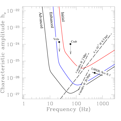
FIG. 3.: Characteristic amplitudes $h_{c}$ [see Eq. (3.5) in [1]] for several postulated periodic sources, compared with sensitivities $h_{\rm 3/yr}$ of the initial, enhanced and advanced detectors in LIGO. ($h_{\rm 3/yr}$ corresponds to the amplitude $h_{c}$ of the weakest source detectable with 99% confidence in $\frac{1}{3}{\rm yr}=10^{7}\mbox{\rm s}$ integration time, if the frequency and phase of the signal, as measured at the detector, are known in advance.) Long-dashed lines show the expected signal strength as a function of frequency for pulsars at a distance of 8.5 kpc assuming a gravitational ellipticity $\epsilon=10^{-5}$ of the source (see Ref. [1]). Upper limits are plotted for the Crab and Vela pulsars, assuming their entire measured spindown is due to gravitational wave emission. The characteristic amplitude of waves from $r$-modes is also shown. These signals are not precisely periodic; rather, they chirp downward through a frequency band of $\sim 200$ Hz in $2\times 10^{7}$ seconds. Finally, the strength of the gravitational waves from LMXB’s, normalized to the observed x-ray flux from Sco X-1, is plotted under the assumption that gravitational waves are entirely responsible for their angular momentum loss.

D Results

The sensitivity $\Theta=1/h_{\mathrm{th}}$ of a search is defined in Eq. (38). The threshold strain amplitude $h_{\mathrm{th}}$ is defined such that there is a 1% a priori probability that detector noise alone will produce an event during the analysis, and therefore is the minimum characteristic strain detectable in the search. We compare our results for the sensitivity $\Theta$ to a canonical sensitivity determined by the search threshold $h_{\mathrm{3/yr}}=4.2\sqrt{S_{n}(f)\times 10^{-7}\mathrm{Hz}}$. This threshold is the characteristic amplitude of the weakest source detectable with $99\%$ confidence in a coherent search of $10^{7}$ seconds of data, if the frequency and phase evolution of the signal are known. The relative sensitivity $\Theta_{\mathrm{rel}}$ is given by $\Theta_{\mathrm{rel}}\equiv h_{\mathrm{3/yr}}/h_{\mathrm{th}}$; a relative sensitivity $\Theta_{\mathrm{rel}}=0.1$ for a search means that a signal must have a characteristic amplitude $h_{c}\gtrsim 10\times h_{\mathrm{3/yr}}$ to be detected in that search. Figure 3 shows $h_{\mathrm{3/yr}}$ based on noise spectral estimates for three detector systems in LIGO: the initial detectors are expected to go on-line in the year 2000, with the first science run from 2002–2004; the upgrade to the enhanced detectors should begin in $\sim$2004, with subsequent upgrades leading to, and perhaps past, the advanced detector sensitivity. The expected amplitudes $h_{c}$ of several putative sources are also shown; we use the definition of $h_{c}$ given in Eq. (50) of Ref. [27], and Eq. (3.5) of Paper I. The strengths of gravitational waves from the Crab and Vela radio pulsars are upper limits assuming all the rotational energy is lost via gravitational waves. The estimates of waves from the r-mode instability are based on Owen et al. [23], and those from Sco X-1 are based on the recent analysis by Bildsten [24].

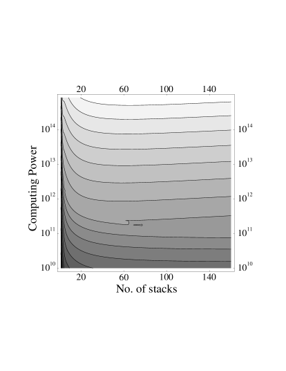
FIG. 4.: A contour plot of the relative sensitivity defined in Sec. I D as a function of available computing power, and the number of stacks in the search. The plot indicates the sensitivity that can be achieved using a stack-slide search for sources with $f\leq 1000$ Hz and $\tau\geq 40$ yr. The darkest shading represents the worst sensitivity. For fixed number of stacks the sensitivity improves with increasing computing power as expected. Notice that for fixed computing resources there is generally a point of optimal sensitivity; indeed the number of stacks at this optimal operating point should be compared with those given in Fig. 7. It is important to notice that the maximum falls off very slowly as the number of stacks increases.

A reasonable long-term search strategy is that data analysis should proceed at roughly the same rate as data acquisition. Given finite computational resources and a desired overall false alarm probability, there is an optimal choice for the length of a data stretch, and the number of stacks that one should analyze in a given search run. The optimal strategy is that which maximizes the final sensitivity of a search subject to the constraints on computational resources and time to analyze the data. We have plotted the relative sensitivity of a search for young, fast pulsars as a function of the number of stacks and the available computing power in Fig. 4. The optimal number of stacks is easily read off the plot for fixed computing power. Note that the maximum sensitivity in this plot is quite flat, especially in the regime where one is most computationally bound. This may be extremely relevant when implementing these search techniques; data management issues may impose more severe constraints on the size and number of stacks than computational power does. This remains to be explored when the data analysis platforms have been chosen.

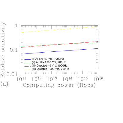
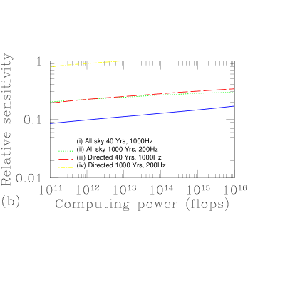
FIG. 5.: Relative amplitude sensitivities $\Theta_{\mathrm{rel}}=h_{\mathrm{3/yr}}/h_{\mathrm{th}}$ achievable with given computational resources, for (a) one pass stack-slide search strategies, and (b) two-pass hierarchical strategies (using the stack-slide algorithm in each pass). The results are presented for our fiducial classes of sources: (i) all-sky search for young ($\tau\geq 40$ yr), fast ($f\leq 1000$ Hz) pulsars, (ii) all-sky search for old($\tau\geq 1000$ yr), slow ($f\leq 200$ Hz) pulsars, (iii) directed search for young, fast pulsars, and, (iv) directed search for old, slow pulsars. For a given computational power, we have determined the optimum observation time, and number of stacks as described in Secs. IV and VI. Thus $h_{\mathrm{th}}$ is the expected sensitivity of the detector for an optimal stack-slide search, with 99% confidence.

Figure 5(a) shows the optimal sensitivities which can be achieved, as a function of available computing power, using a stack-slide search. The results are presented for both fiducial classes of pulsars: old ($\tau\geq 1\,000$ yr) slow ($f\leq 200$ Hz) pulsars, and young ($\tau\geq 40$ yr) fast ($f\leq 1\,000$ Hz) pulsars. In each case, we have considered both directed and all-sky searches for the sources. The results should be compared with those of Paper I, in which we considered coherent searches without stacking: the use of stacked searches gains a factor of $\sim$2–4 in sensitivity.

The use of a two-pass hierarchical search can further improve sensitivities by balancing the computational requirements between the two passes. Figure 5(b) shows the sensitivities achievable when each pass uses a stack-slide strategy. The sensitivities achieved exceed those of one-pass stack-slide searches by $\sim 20$–$60$%.

The computational requirements for all-sky, all frequency surveys are sufficiently daunting that we explore three restricted searches in Sec. VII: (i) a directed search for a newborn neutron star in the young ($\lesssim 1$ year old) remnant of an extra-galactic supernova, (ii) an area search of the galactic core for pulsars with $\tau\geq 100\>\textrm{yr}$ and $f\leq 500\>\textrm{Hz}$, and (iii) a directed search for an accreting neutron star in a binary system (such as Sco X-1). Figure 6 shows the relative sensitivities attainable in such searches. With computational resources capable of $1$ Tflops, we expect to see galactic core pulsars with enhanced LIGO if they have non-axisymmetric strains of $\epsilon\gtrsim 5\times 10^{-6}$ at frequencies of $\sim 200$ Hz. Estimates of the characteristic strain of gravitational waves from an active $r$-mode instability in a newborn neutron star suggest that these sources will be detectable by the enhanced interferometers in LIGO out to distances $\sim 8$ Mpc; the rate of supernovae is $\sim 0.6$ per year within this distance. Finally, gravitational waves from accreting neutron stars in low-mass x-ray binary systems (LMXBs) may be detectable by enhanced interferometers in LIGO if we can obtain sufficient information about the binary orbit from electromagnetic observations. Sco X-1 is on the margins of detectability using the enhanced LIGO interferometers operating in broadband configuration. We estimate that the amplitude signal-to-noise from these sources could be improved by a factor of $\sim 5$–$10$ by operating the interferometer in a signal-recycled, narrow-band configuration.

E Organization of the paper

In Sec. II we extend the metric formalism that was developed in Paper I to determine the number of parameter space points that must be sampled in a search that accumulates signal to noise by summing up power spectra. This method can then be used to compute the number of correction points needed in a stack-slide search. Approximate formulae, useful for estimating the computational cost of a search, are presented for the number of corrections needed in an all-sky search, and also in directed searches of a single sky position.

We discuss the the issue of thresholding in Sec. III. Then we present the computational cost estimates, and determine the optimal parameters for single-pass, stack-slide searches in Sec. IV

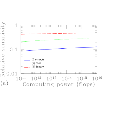
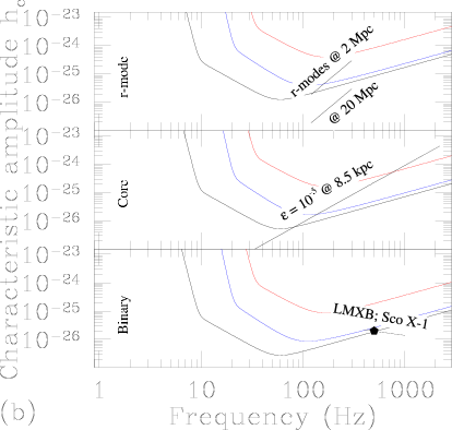
FIG. 6.: Panel (a) represents the relative amplitude sensitivities $\Theta_{\mathrm{rel}}=h_{\mathrm{3/yr}}/h_{\mathrm{th}}$ achievable with given computational resources, in three specialized searches: (i) A search for a new-born neutron star (whose direction is determined by observing an optical supernova) that is spinning down by gravitational wave emission via an active $r$-mode instability. We took $\tau\geq 1$ yr and $f\leq 200$ Hz. (ii) A search for pulsars in a region extending $0.004$ steradians about the galactic core, with $\tau\geq 100$ yr and $f\leq 500$ Hz. (iii) A source in a binary orbit, e.g. Sco X-1. We assume the orbit is characterized by two orthogonal velocity parameters, known to within a total error of $17(\mathrm{km/s})^{2}$; we further assume that the frequency $f\leq 500$ Hz experiences a random walk typical of Eddington-rate accretion. For each of these sources, panel (b) shows $h_{\mathrm{th}}$ for initial (upper lines), enhanced (middle lines), and advanced (lower lines) interferometers in LIGO, assuming $1$ Tflops of computing power. Thus this is the characteristic amplitude of the weakest source that can be detected with $99\%$ confidence using a two pass-hierarchical search strategy.

Section V presents a general discussion of hierarchical searches for periodic sources using a single interferometer. Schutz [28] has previously considered hierarchical searches demonstrating their potential in searches for periodic sources. The relationship between the threshold in the second stage of the search, and the threshold required in the first stage is discussed in detail. We also present the computational cost of each stage of the search. These results are used in Sec. VI to determine the optimal search parameters in hierarchical searches for our fiducial classes of sources.

Finally, we discuss three specialized searches in Sec. VII. We present a preliminary investigation of issues which arise when the gravitational wave source is in a binary system (e.g. an LMXB). We discuss a parameterized model of the binary orbit, and estimate the number of parameter space points which must be sampled in a search for the gravitational waves from one of the objects in the binary. In the case where the emitter is accreting material from its companion, we also allow for stochastic changes in frequency due to fluctuations in the accretion rate.

Detailed formulae for the number of points in parameter space when dealing with a stacked search are presented in Appendix A. In Appendix B we discuss the loss in signal to noise that can occur when using nearest neighbor resampling to apply corrections to the detector output. If the data is sampled at $16\,384$ Hz, we demonstrate that this method will lose less than $1\%$ of amplitude signal-to-noise for a signal with gravitational wave frequency $\leq 1000$ Hz,

II Mismatch

In a detection strategy that searches over a discrete mesh of points in parameter space, the search parameters and signal parameters will never be precisely matched. This mismatch will reduce the signal to noise since the signal will not be precisely monochromatic. It is desirable to quantify this loss, and to choose the grid spacing so that the loss is within acceptable limits. This can be achieved by defining a distance measure on the parameter space based on the fractional losses in detected signal power due to parameter mismatch. In Paper I we derived such a measure in the case where the search was performed using coherent Fourier transforms; this method was modeled after Owen’s computation of a metric on the parameter space of coalescing binary waveforms [29]. In this paper we extend this approach to the case of incoherent searches, in which several power spectra are added incoherently, or stacked, and then searched for spikes.

Let $h(t;\mbox{\boldmath${\lambda}$\unboldmath})$ be a hypothetical signal given by Eq. (4) with true signal parameters $\mbox{\boldmath${\lambda}$\unboldmath}=(f_{0},\vec{\lambda})$. If the data containing this signal are corrected for some nearby set of shape parameters $\vec{\lambda}+\Delta\vec{\lambda}$, the signal will take the form

$$h_{b}(t;\mbox{\boldmath${\lambda}$\unboldmath},\Delta\mbox{\boldmath${\lambda}$\unboldmath})={\cal A}e^{-i\{2\pi f_{0}t_{b}[t;\vec{\lambda}]+\phi[t;\mbox{\boldmath${\lambda}$\unboldmath}]-\phi[t;(f_{0},\vec{\lambda}+\Delta\vec{\lambda})]\}}\;,$$ (8)

where the subscript $b$ is used to indicate the corrected waveform. In a stacked search, the data are divided into $N$ segments of equal length $\Delta T$, each of these segments is Fourier transformed, and then a total power spectrum $P_{h}(f;\mbox{\boldmath${\lambda}$\unboldmath},\Delta\vec{\lambda})$ is computed according to the formula

$$H(f;\mbox{\boldmath${\lambda}$\unboldmath},\Delta\vec{\lambda})=2\sum_{k=1}^{N}|\tilde{h}_{k}(f;\mbox{\boldmath${\lambda}$\unboldmath},\Delta\vec{\lambda})|^{2}\;.$$ (9)

The Fourier transform of each individual segment is defined to be

$$\tilde{h}_{k}(f;\mbox{\boldmath${\lambda}$\unboldmath},\Delta\vec{\lambda})=\frac{\cal A}{\sqrt{\Delta T}}\int_{(k-1)\Delta T}^{k\Delta T}e^{i\Delta\phi[t;\mbox{\boldmath${\lambda}$\unboldmath},\Delta\mbox{\boldmath${\lambda}$\unboldmath}]}\;dt_{b}$$ (10)

where $\Delta\phi$ is given by

$$\Delta\phi[t;\mbox{\boldmath${\lambda}$\unboldmath},\Delta\mbox{\boldmath${\lambda}$\unboldmath}]=2\pi(f-f_{0})t_{b}+\phi[t;(f_{0},\vec{\lambda}+\Delta\vec{\lambda})]-\phi[t;\mbox{\boldmath${\lambda}$\unboldmath}]\;.$$ (11)

Here $\Delta\mbox{\boldmath${\lambda}$\unboldmath}=(f-f_{0},\Delta\vec{\lambda})$ denotes the error in matching the modulation shape parameters and the error in sampling the resulting power spectrum at the wrong frequency. Both of these errors lead to a reduction in the detected power relative to the optimum case where the carrier frequency and the phase modulation are precisely matched.

The mismatch $m(\mbox{\boldmath${\lambda}$\unboldmath},\Delta\mbox{\boldmath${\lambda}$\unboldmath})$, which is the fractional reduction in power due to imperfect phase correction and sampling at the wrong Fourier carrier frequency, is defined to be

$$m(\mbox{\boldmath${\lambda}$\unboldmath},\Delta\mbox{\boldmath${\lambda}$\unboldmath})=1-\frac{H(f;\mbox{\boldmath${\lambda}$\unboldmath},\Delta\vec{\lambda})}{H(f_{0};\mbox{\boldmath${\lambda}$\unboldmath},\vec{0})}\;.$$ (12)

Remember $\mbox{\boldmath${\lambda}$\unboldmath}=(\lambda_{0},\vec{\lambda})=(f,\lambda_{1},\lambda_{2}\ldots)$. Substituting the expressions for $H$ from Eq. (9) into Eq. (12), we find

$$m(\mbox{\boldmath${\lambda}$\unboldmath},\Delta\mbox{\boldmath${\lambda}$\unboldmath})=1-\frac{1}{N{\cal A}^{2}}\sum_{k=1}^{N}|\tilde{h}_{k}(f;\mbox{\boldmath${\lambda}$\unboldmath},\Delta\vec{\lambda})|^{2}\;.$$ (13)

It is easily shown that $m(\mbox{\boldmath${\lambda}$\unboldmath},\Delta\mbox{\boldmath${\lambda}$\unboldmath})$ has a local minimum of zero when $\Delta\mbox{\boldmath${\lambda}$\unboldmath}=0$. We therefore expand the mismatch in powers of $\Delta\mbox{\boldmath${\lambda}$\unboldmath}$ to find

$$m(\mbox{\boldmath${\lambda}$\unboldmath},\Delta\mbox{\boldmath${\lambda}$\unboldmath})=\sum_{\alpha,\beta}g_{\alpha\beta}(\mbox{\boldmath${\lambda}$\unboldmath})\Delta\lambda^{\alpha}\Delta\lambda^{\beta}+{\cal O}(\Delta\mbox{\boldmath${\lambda}$\unboldmath}^{3})\;,$$ (14)

where $(\alpha,\beta)$ are summed over $0,1,\ldots,j,\ldots$. The quantity $g_{\alpha\beta}$ is a local distance metric on the parameter space. This metric is explicitly given by

$$g_{\alpha\beta}(\mbox{\boldmath${\lambda}$\unboldmath})\equiv{\textstyle\frac{1}{2}}\partial_{\Delta\lambda^{\alpha}}\partial_{\Delta\lambda^{\beta}}m(\mbox{\boldmath${\lambda}$\unboldmath},\Delta\mbox{\boldmath${\lambda}$\unboldmath})|_{\Delta\mbox{\boldmath${\lambda}$\unboldmath}=0}\;,$$ (15)

where $\partial_{\Delta\lambda^{\alpha}}$ denotes a partial derivative with respect to $\Delta\lambda^{\alpha}$. It is convenient to express $g_{\alpha\beta}$ as a sum of metrics computed for the individual stacks, that is

$$g_{\alpha\beta}(\mbox{\boldmath${\lambda}$\unboldmath})=\frac{1}{N}\sum_{k=1}^{N}g_{\alpha\beta}^{(k)}(\mbox{\boldmath${\lambda}$\unboldmath})$$ (16)

where the individual stack metrics $g_{\alpha\beta}^{(k)}(\mbox{\boldmath${\lambda}$\unboldmath})$ are explicitly given by

$$g_{\alpha\beta}^{(k)}(\mbox{\boldmath${\lambda}$\unboldmath})=\langle\partial_{\Delta\lambda^{\alpha}}\Delta\phi\,\partial_{\Delta\lambda^{\beta}}\Delta\phi\rangle_{k}-\langle\partial_{\Delta\lambda^{\alpha}}\Delta\phi\rangle_{k}\langle\partial_{\Delta\lambda^{\beta}}\Delta\phi\rangle_{k}\;.$$ (17)

The phase error $\Delta\phi$ is given in Eq. (11), and we use the notation

$$\langle\ldots\rangle_{k}=\left.\frac{1}{\Delta T}\int_{(k-1)\Delta T}^{k\Delta T}(\ldots)dt_{b}\right|_{\Delta\mbox{\boldmath${\lambda}$\unboldmath}=0}\;.$$ (18)

In a search, we will look for spikes in the power spectrum $H(f;\mbox{\boldmath${\lambda}$\unboldmath},\Delta\vec{\lambda})$ computed from the detector output, that is, we will look for local maxima in the frequency parameter $f$. Therefore the relevant measure of distance in the space of shape parameters $\vec{\lambda}$ is the fractional loss in power due to mismatched parameters $\Delta\vec{\lambda}$, but after maximizing over frequency. We therefore define the projected mismatch $\mu(\vec{\lambda},\Delta\vec{\lambda})$ to be

$$\mu(\vec{\lambda},\Delta\vec{\lambda})=\min_{f}m(\mbox{\boldmath${\lambda}$\unboldmath},\Delta\mbox{\boldmath${\lambda}$\unboldmath})=\sum_{i,j}\gamma_{ij}(\vec{\lambda})\Delta\lambda^{i}\Delta\lambda^{j}\;,$$ (19)

where

$$\gamma_{ij}=\left(g_{ij}-\frac{g_{i0}g_{j0}}{g_{00}}\right)_{\lambda^{0}=f_{\mathrm{max}}}$$ (20)

is the mismatch metric projected onto the subspace of shape parameters, and $f_{\mathrm{max}}$ is the maximum frequency that we include in the search. The meaning of the minimization $\min_{f}$ is clear from the definition of the mismatch in Eq. (13).

The distance function, and in particular the metric in Eq. (20), can be used to determine the number of discrete mesh points that must be sampled in a search. Let $\cal P$ be the space of all parameter values $\vec{\lambda}$ to be searched over, and define the maximal mismatch $\mu_{\mathrm{max}}$ to be the largest fractional loss of power that we are willing to tolerate from a putative source with parameters in $\cal P$. For the model waveform in Eqs. (1), (2), and (4) this parameter space is coordinatized by $\vec{\lambda}=(\theta,\phi,f_{1},f_{2},\ldots)$ where $\theta$,$\phi$ denote location of the source on the sky, and $f_{j}$ are related to the time derivative of the intrinsic frequency of the source. Each correction point of the mesh is considered to be at the center of a cube with side $2\sqrt{\mu_{\mathrm{max}}/n}$, where $n$ is the dimension of $\cal P$; this insures that all points in $\cal P$ are within a proper distance $\mu_{\mathrm{max}}$ of a discrete mesh point as measured with the metric $\gamma_{ij}$. The number of patches required to fill the parameter space is

$$N_{p}(\Delta T,\mu_{\mathrm{max}},N)=\frac{\int_{\cal P}\sqrt{\det|\gamma_{ij}|}d^{n}\lambda}{(2\sqrt{\mu_{\mathrm{max}}/n})^{n}}\;.$$ (21)

Since $\mu_{\mathrm{max}}$ is the maximum loss in detected power after the power spectra have been added, $N_{p}(\Delta T,\mu_{\mathrm{max}},N)$ is the number of patches required to construct the fine mesh in the stacked search strategy described in Sec. I C. The coarse mesh in the stacked search strategy requires only that the spikes in the individual power spectra be reduced by no more than $\mu_{\mathrm{max}}$; consequently, the number of points in such a mesh is simply $N_{p}(\Delta T,\mu_{\mathrm{max}},1)$.

We note that the average expected power loss for a source randomly placed within such cubical patches is $\langle\mu\rangle=\mu_{\mathrm{max}}/3$. (In Paper I we quoted an average that was computed for ellipsoidal patches; this is not appropriate to the cubical grid which will likely be used in a real search.)

A Directed search

In most cases, the forms of Eqs. (2) and (6) are sufficiently complicated to defy analytical solution, especially since $\vec{v}$ in Eq. (2) should properly be taken from the true ephemeris of the Earth during the period of observation. However, for the case of a directed search, that is a search in just a single sky direction, the phase correction is polynomial in $t$, and the metric can be computed analytically. To a good approximation, the metric is flat — the spacing of points in parameter space is independent of the value of the spindown parameters $(f_{1},f_{2},\ldots,f_{s})$. For a given number $s$ of spindown parameters in a search, the right hand side of Eq. (21) can be evaluated analytically. The result is expressed as a product ${\cal N}_{s}{G}_{s}$, where

$${\cal N}_{s}=\frac{f_{\mathrm{max}}^{s}(\Delta T)^{s(s+3)/2}}{(\mu_{\mathrm{max}}/s)^{s/2}\tau_{\mathrm{min}}^{s(s+1)/2}}\;$$ (22)

depends on the maximum frequency $f_{\mathrm{max}}$ (in Hz), the length of each stack $\Delta T$ (in seconds), the maximal mismatch $\mu_{\mathrm{max}}$, and the minimum spindown age $\tau_{\mathrm{min}}$ (in seconds) to be considered in the search. The dependence on the number of stacks $N$ is contained in $G_{s}(N)$ which are given by:

$$G_{0}(N) = 1\;,$$ (23)

$$G_{1}(N) \approx 0.524N\;,$$ (24)

$$G_{2}(N) \approx 0.0708N^{3}\;,$$ (25)

$$G_{3}(N) \approx 0.00243N^{6}\;,$$ (26)

when $N\gg 4$. The detailed expressions for $G_{s}(N)$ are presented in Appendix A. For up to $3$ spindown terms in the search, the number of patches is then

$$N_{p}(\Delta T,\mu_{\mathrm{max}},N)=\max_{s\in\{0,1,2,3\}}[{\cal N}_{s}G_{s}(N)]\;.$$ (27)

The maximization accounts for the situation where increasing $s$, the dimension of the parameter space, decreases the value of ${\cal N}_{s}G_{s}$ because the parameter space extends less than one patch width in the new spindown coordinate $f_{s}$; one should not search over this coordinate.

B Sky search

For signal modulations that are more complicated than simple power-law frequency drift, it is impossible to compute $N_{p}$ analytically. In an actual search over sky positions as well as spindown, one should properly compute the mismatch metric numerically, using the exact ephemeris of the Earth in computing the detector position. In Paper I we computed $N_{p}(T_{b},\mu_{\mathrm{max}},1)$ numerically, with the simplification that both the Earth’s rotation and orbital motion were taken to be circular. However, in this paper we are concerned also with the dependence of $N_{p}$ on the number of stacks $N$. This significantly complicates the calculation of the metric and its determinant, and makes it necessary to adopt some approximations in the calculation. Fortunately, the results of interest here are rather insensitive to errors in $N_{p}$.

In Paper I we mentioned that there are strong correlations between sky position and spindown parameters, thus requiring the use of the full $s+2$ dimensional metric. However, these correlations are due primarily to the Earth’s orbital motion, to which a low-order Taylor approximation is good for times much less than a year. Therefore we treat the number of patches as the product of the number of spindown patches times the number of sky positions ${\cal M}_{s}$, computed analytically using only the Earth’s rotational motion. We note that this approximation is appropriate only for computing the number of patches; when actually demodulating the signals, the true orbital motion would have to be included. This approximation works well so long as the orbital residuals (the remaining orbital modulations after correction on this sky mesh) are much smaller than the spindown corrections being made at the same power in $t$. The residual orbital velocity at any power $t^{k}$ is roughly

$$\sim\frac{\alpha_{k}}{k!\sqrt{{\cal M}_{s}}}\times\frac{r\Omega}{c}\times(\Omega t)^{k}\;,$$ (28)

where $\alpha_{k}$ is a number of order unity, ${\cal M}_{s}$ is the number of sky patches, and $r=1$AU and $\Omega=2\pi$/yr are the Earth’s orbital radius and angular velocity. When the range in this residual is comparable to or larger than the range in the corresponding spindown term $f_{k}t^{k}$, the “spindown” parameter space must be expanded to include the orbital residuals. While the range in $\alpha_{k}$ is difficult to arrive at analytically, we have found that assuming a maximum value of $\approx 0.3$ gives good agreement with the numerical results of Paper I (i.e. for $N=1$), to within factors of $\sim 2$.

One other approximation was made in computing the number of sky patches. We found that the measure $\sqrt{\det|\gamma_{ij}|}$ for the sky position metric is almost constant in the azimuth $\varphi$, and has a polar angle dependence which is dominantly of the form $\sin 2\theta$. When performing the integral over sky positions, we approximated the measure by $\sqrt{\det|\gamma_{ij}|}\simeq\textrm{constant}\times\sin 2\theta$; this approximation is accurate to about one part in $10^{4}$.

Given these approximations, the number of patches for a sky search is given by:

$$N_{p}=\max_{s\in\{0,1,2,3\}}\left[{\cal M}_{s}\overline{{\cal N}}_{s}G_{s}\prod_{k=0}^{s}\left(1+\frac{0.3r\Omega^{k+1}\tau_{\mathrm{min}}^{k}}{c\,k!\sqrt{{\cal M}_{s}}}\right)\right]\;.$$ (29)

The number of sky patches ${\cal M}_{s}$, in the $(s+2)$-dimensional search, is given approximately by

$${\cal M}_{s} \approx \frac{f_{\mathrm{max}}^{2}}{4\mu_{\mathrm{max}}/(s+2)}\left(A^{-2}+B^{-2}+C^{-2}\right)^{-1/2}\;,$$ (30)

$$A = 0.014\;,$$ (31)

$$B = 0.046(\Delta T/1\,\mathrm{day})^{2}\;,$$ (32)

$$C = 0.18(\Delta T/1\,\mathrm{day})^{5}N^{3}\;.$$ (33)

This is a fit to the analytic result given in Appendix A. The number of spindown patches $\overline{{\cal N}}_{s}G_{s}$ in the $(s+2)$-dimensional search is

$$\overline{{\cal N}}_{s}G_{s}=\frac{s^{s/2}}{(s+2)^{s/2}}{{\cal N}}_{s}G_{s}\;$$ (34)

where ${{\cal N}}_{s}$ and $G_{s}$ are given in Eqs. (22)–(26), and the prefactor on the right corrects for the sky dimensions. The remaining product terms $\prod$ in Eq. (29) represent the increase in the size of the spindown space in order to include the orbital residuals.

III Thresholds and sensitivities

The thresholds for a search are determined under the assumption that the detector noise is a stationary, Gaussian random process with zero mean and power spectral density $S_{n}(f)$. In the absence of a signal, the power $P_{n}(f)=2|\tilde{n}(f)|^{2}$ at each sampled frequency is exponentially distributed with probability density function $e^{-P_{n}/S_{n}}/S_{n}$. The statistic for stacked spectra is $\rho=\sum_{1}^{N}P_{n}(f)$. The cumulative probability distribution function for $\rho$, in the absence of a signal, is

$$\textrm{CDF}[\rho/S_{n},N]=\int_{0}^{\rho/S_{n}}e^{-r}\frac{r^{N-1}}{(N-1)!}\;dr=\frac{\gamma(N,\rho/S_{n})}{(N-1)!}$$ (35)

where $\gamma(N,\rho/S_{n})$ is an incomplete gamma function.

A (candidate) detection occurs whenever $\rho$ in some frequency bin exceeds a pre-specified threshold $\rho_{c}$ chosen so that the probability of a false trigger due to noise alone is small. There are $f_{\mathrm{max}}\Delta T$ Fourier bins in each spectrum, and $N_{p}(\Delta T,\mu_{\mathrm{max}},N)$ spectra in the entire search. Therefore we assume that a search consists of $N_{p}f_{\mathrm{max}}\Delta T$ independent trials of the statistic $\rho$, and compute the expected number of false events $F$ to be

$$F=f_{\mathrm{max}}\Delta T\,N_{p}(\Delta T,\mu_{\mathrm{max}},N)\,(1-\textrm{CDF}[\rho_{c}/S_{n},N])\;.$$ (36)

(In reality, there will be correlations between the statistic computed for different frequencies and different patches. Since this will reduce the number of independent trials, Eq. (36) overestimates the number of false events. This is a small effect which should not change the overall sensitivity of a search by much. It is only in the case that the number of trials is initially small that one should be concerned with this effect; unfortunately, we operate in the other extreme.) If $F\ll 1$, number of false events $F$ is approximately equal to the probability that an event is caused by noise in the detector. Consequently, $\alpha=1-F$ can be thought of as our confidence of detection. In a non-hierarchical search, the threshold $\rho_{c}$ is set by specifying $\alpha$ and then inverting Eq. (36).

Finally, how does the threshold $\rho_{c}$ affect the sensitivity of our search? We define a threshold amplitude $h_{\mathrm{th}}$ to be the minimum dimensionless signal amplitude that we expect to register as a detection in the search

$$h_{\mathrm{th}}=\sqrt{\frac{(\rho_{c}/N-S_{n})}{\langle F_{+}^{2}(\Theta,\Phi,\Psi)\rangle(1-\langle\mu\rangle)\Delta T}}$$ (37)

where $\langle F_{+}^{2}(\Theta,\Phi,\Psi)\rangle$ is the square of the detector response averaged over all possible source positions and orientations, and $\langle\mu\rangle=\mu_{\mathrm{max}}/3$ is the expected mismatch of a signal which is randomly located within a patch. The sensitivity $\Theta$ of the search is then defined by

$$\Theta\equiv\frac{1}{h_{\mathrm{th}}}\propto\sqrt{\frac{(1-\mu_{\mathrm{max}}/3)\Delta T}{\rho_{c}/N-S_{n}}}\;.$$ (38)

For any optimal search strategy, the goal of optimization will be to maximize the final sensitivity of the search, given limited computational power.

IV Stack-slide search

A stack-slide search is the simplest alternative to coherent searches we consider here. The main steps involved in the algorithm are shown in the flow chart of Fig. 1. In this section we estimate the computational cost of each step, and determine the ultimate sensitivity of this technique.

The first step, before the search begins, is to specify the size of the parameter space to be searched (i.e. choose $f_{\mathrm{max}}$, $\tau$, and a region of the sky), the computational power $P$ that will be available to do the data analysis, and an acceptable false alarm probability. From these, one can determine optimal values for the maximum mismatch $\mu_{\mathrm{max}}$ for a patch, the number of stacks $N$, and the length $\Delta T$ of each stack, using the optimization scheme discussed at the end of this section. For now, we treat these as free parameters.

Coarse and fine grids are laid down on the parameter space with $N_{pc}=N_{p}(\Delta T,\mu_{\mathrm{max}},1)$ and $N_{pf}=N_{p}(\Delta T,\mu_{\mathrm{max}},N)$ points, respectively. The data-stream is low-pass filtered to the upper cutoff frequency $f_{\mathrm{max}}$, and broken into $N$ stretches of length $\Delta T$. Each of the steps above have negligible computational cost since they are done only once for the entire search. The subsequent steps, on the other hand, must be executed for each of the $N_{pc}$ correction points.

Each stretch of data is re-sampled (at the Nyquist frequency $2f_{\mathrm{max}}$) and simultaneously demodulated by stroboscopic sampling for a set of demodulation parameters selected from the coarse grid. The result is $N$ demodulated time series, each one consisting of $n=2f_{\mathrm{max}}\Delta T$ samples. Since stroboscopic demodulation only shifts one in every few thousand data points (assuming a sampling rate at the detector of $16\,384\>\mathrm{Hz}$), the computational cost of the demodulation itself is negligible.

Each stretch of data is then Fourier transformed using a fast Fourier transform (FFT) algorithm with a computational cost of $3nN\log_{2}(n)$ floating point operations. Power spectra are computed for each Fourier series, costing 3 floating point operations per frequency bin, i.e., a total cost of $1.5nN$ floating point operations.

For demodulation parameters in the coarse grid, the power of a matched signal will be confined to $\sim 1$ Fourier bin in each power spectrum, but not necessarily the same bin in different spectra. To insure that power from a signal is accumulated by summing the $N$ spectra, we must apply $N_{pf}/N_{pc}$ corrections within each coarse mesh patch. This can be achieved by the following steps.

For the $N$ spectra to be stacked, the frequency of a putative signal with initial frequency $f_{\mathrm{max}}$ is computed using Eq. (1). Each spectrum is re-indexed so that the power from such a signal would be in the same frequency bin (we ignore the computational cost of this step), and the spectra are added [$0.5n(N-1)$ floating point operations]. We automatically account for corrections at other frequencies by applying the fine grid corrections in this way. It may be possible to reduce the computational cost of this portion of the search by noting, for example, that we over count the fine grid corrections for signals with frequency $f_{\mathrm{max}}/2$ by a factor of $2^{n}$ where $n$ is the dimension of the parameter space being explored. Since it is difficult to assess the feasibility of using this in a real search, we simply mention it so that it might be explored at the time of implementation.

The resulting stacked spectrum is scanned for peaks which exceed the threshold $\rho_{c}$. Since this has negligible computational cost, the number of floating point operations required for the entire search is

$$C=3nNN_{pc}\,[\log_{2}(n)+0.5+N_{pf}(N-1)/(6NN_{pc})]\;.$$ (39)

If data analysis proceeds at the same rate as data acquisition, the computational power $P$ required to complete a search is $P=C/N\Delta T$ floating-point operations

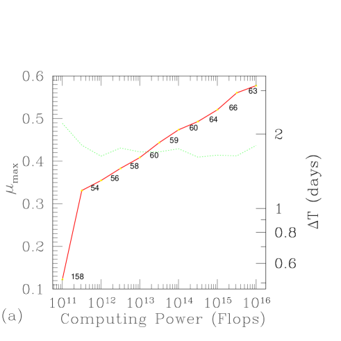
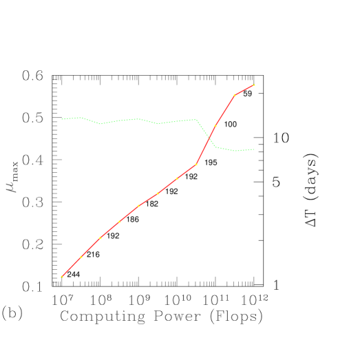
FIG. 7.: The optimum stack length $\Delta T$ (thick solid line), number of stacks $N$ (numbers along the solid line), and maximal projected mismatch $\mu_{\mathrm{max}}$ (dotted line) as functions of available computational power for directed, stack-slide searches. The two panels correspond to the following cases: (a) The situation encountered when searching for periodic sources having gravitational wave frequencies up to $1000\mbox{\rm Hz}$, with minimum spindown ages $\tau_{\rm min}=40\mbox{\rm yr}$. (b) The equivalent results for gravitational wave frequencies up to $200\mbox{\rm Hz}$, with minimum spindown ages $\tau_{\rm min}=10^{3}\mbox{\rm yr}$. Both cases assume a threshold which gives an overall statistical significance of $99\%$ to a detection (although the results are insensitive to the precise value). The optimization was performed numerically using simulated annealing which accounts for some of the fluctuations in the observation times.

per second (Flops). Equation (39) and the definition of $n=2f_{\mathrm{max}}\Delta T$ imply that the computational power is

$$P=6f_{\mathrm{max}}N_{pc}\,[\log_{2}(n)+0.5+N_{pf}(N-1)/(6NN_{pc})]\;.$$ (40)

The final sensitivity $\Theta$, defined in Eq. (38), of the search is determined once we know the function $N_{p}$, the

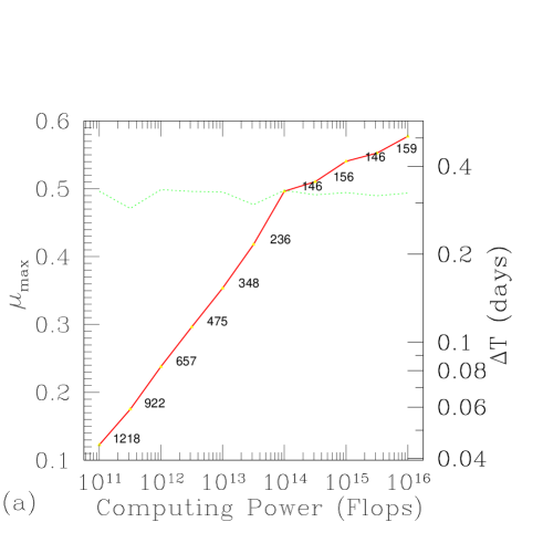
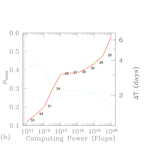
FIG. 8.: Same as in Fig. 7, but for an all-sky search.

frequency $f_{\mathrm{max}}$, the maximal mismatch $\mu_{\mathrm{max}}$, and the confidence level $\alpha=1-F$. An optimized algorithm will maximize $\Theta$ as a function of $\mu_{\mathrm{max}}$, $N$, and $\Delta T$, subject to the constraints imposed by fixing the false alarm probability $F$, and the computational power $P$.

The results of the optimization procedure are given in Figures 7 and 8 for the fiducial classes of pulsar defined in Sec. I B. In each case we have set the probability of a false alarm threshold at $F=0.01$ (indicating a 99% confidence that detector noise will not produce an event above threshold), and have determined optimal values of $\mu_{\mathrm{max}}$, $N$, and $\Delta T$ for a range of values of the available computational power. Figures 7(a) and (b) show the results for a directed search for old, slow ($\tau_{\mathrm{min}}$=1 000 yr, $f_{\mathrm{max}}$=200 Hz) and young, fast ($\tau_{\mathrm{min}}$=40 yr, $f_{\mathrm{max}}$=1 000 Hz) pulsars, respectively. Figures 8(a) and (b) show the results for an all-sky search for the same two classes of source. The optimal sensitivities achieved by these searches are summarized in Fig. 5(a) of the Introduction.

V Hierarchical search: general remarks

The basic hierarchical strategy involving a two pass search is represented schematically in Fig. 2. In the first pass, $N^{(1)}$ stacks of data of length $\Delta T^{(1)}$ are demodulated on a coarse and fine mesh of correction points computed for some mismatch level $\mu^{(1)}$, and then searched by stacked Fourier transforms. A threshold signal-to-noise level is chosen which will, in general, admit many false alarms. In the second stage, $N^{(2)}$ stacks of length $\Delta T^{(2)}$ are searched on a finer mesh of points computed at a mismatch level $\mu^{(2)}$, but only in the vicinity of those events which passed the first-stage threshold. The second stage will involve fewer correction points than the first, so the second-stage transforms can be made longer and more sensitive. The goal of optimization is to find some combination of $\Delta T^{(1)}$, $\Delta T^{(2)}$, $\mu^{(1)}$, $\mu^{(2)}$, $N^{(1)}$, and $N^{(2)}$ which maximizes the final sensitivity for fixed computational power $P$, and second pass false alarm probability $F^{(2)}$.

A Thresholds

In the first pass of a hierarchical search, each of $N_{f}^{(1)}=f_{\mathrm{max}}\Delta T^{(1)}$ frequency bins in $N_{pf}^{(1)}=N_{p}(\Delta T^{(1)},\mu^{(1)},N^{(1)})$ stacked power spectra will be scanned for threshold crossing events. If (as we assume) all of these trials are statistically independent, the number of false events above the threshold $\rho^{(1)}$ will be

$$F^{(1)}=N_{pf}^{(1)}N_{f}^{(1)}(1-\textrm{CDF}[\rho^{(1)}/S_{n}^{(1)},N^{(1)}])\;.$$ (41)

We assume that the number of false events will significantly exceed the number of true signals in this pass, consequently the number of events to be analyzed in the second pass will be $F^{(1)}$.

The second stage uses a coarse grid with $N_{pc}^{(2)}=N_{p}(\Delta T^{(2)},\mu^{(2)},1)$ points, and a fine grid with $N_{pf}^{(2)}=N_{p}(\Delta T^{(2)},\mu^{(2)},N^{(2)})$ points. On average each false alarm will require $N_{pc}^{(2)}/N_{pf}^{(1)}$ coarse grid points, and $N_{pf}^{(2)}/N_{pf}^{(1)}$ fine grid points in the second stage. (When a second-pass mesh is coarser than the first pass’s parameter determination, the corresponding ratio should be taken as unity.) Furthermore, since the first stage will identify the candidate signal’s frequency to within $\sim 2$ frequency bins, the second-stage search should be over the $2\Delta T^{(2)}/\Delta T^{(1)}$ second-stage frequency bins which lie in this frequency range. Once again, we assume the noise in all frequency bins (and over all grid points) is independent, so the number of false events which exceed the threshold $\rho^{(2)}$ in the second stage is

$$1-\alpha = F^{(2)}$$ (42)

$$= 2F^{(1)}\frac{N_{pf}^{(2)}}{N_{pf}^{(1)}}\frac{\Delta T^{(2)}}{\Delta T^{(1)}}(1-\textrm{CDF}[\rho^{(2)}/S_{n}^{(2)},N^{(2)}])$$ (43)

$$= 2f_{\mathrm{max}}\Delta T^{(2)}N_{pf}^{(2)}(1-\textrm{CDF}[\rho^{(1)}/S_{n}^{(1)},N^{(1)}])$$ (45)

$$\times(1-\textrm{CDF}[\rho^{(2)}/S_{n}^{(2)},N^{(2)}])\;,$$

where $\alpha$ is our desired confidence level for the overall search.

The thresholds $\rho^{(1)}$ and $\rho^{(2)}$ cannot be assigned independently; rather, they should be chosen so that any true signal buried in the noise that would exceed (in expectation value) the second-stage threshold will have passed the first-stage threshold. In other words, it serves no purpose to set $\rho^{(2)}$ any lower than the weakest signal which would have passed $\rho^{(1)}$. A signal which is expected to pass the second-stage threshold exactly has an amplitude $|\tilde{h}^{(2)}|^{2}=\rho^{(2)}-N^{(2)}S_{n}^{(2)}$. We define the false dismissal probability $D$ to be the probability that such a signal will be falsely rejected in the first pass. Since the spectral power of a true signal increases with $N\Delta T$, the signal seen in the first pass has amplitude $|\tilde{h}^{(1)}|^{2}=|\tilde{h}^{(2)}|^{2}(N^{(1)}\Delta T^{(1)})/(N^{(2)}\Delta T^{(2)})$, and the thresholds satisfy the relation

$$D = \textrm{CDF}\left[\frac{\rho^{(1)}-|\tilde{h}^{(1)}|^{2}}{S_{n}^{(1)}},N^{(1)}\right]$$ (46)

$$= \textrm{CDF}\left[\frac{\rho^{(1)}}{S_{n}^{(1)}}-\left(\frac{\rho^{(2)}}{S_{n}^{(2)}}-N^{(2)}\right)\frac{S_{n}^{(2)}}{S_{n}^{(1)}}\frac{N^{(1)}\Delta T^{(1)}}{N^{(2)}\Delta T^{(2)}},N^{(1)}\right]\;.$$ (47)

Now, for any choice of $\Delta T^{(1)}$, $\Delta T^{(2)}$, etc., the thresholds $\rho^{(1)}$ and $\rho^{(2)}$ are completely constrained by our choices of final confidence level $\alpha$ and false dismissal probability $D$. The false dismissal probability is fixed at $D=0.01$ in our optimization; this is an acceptably low level, meaning that only one signal in a hundred is expected to be lost in this type of search.

B Computational costs

The computational cost $C^{(1)}$ of the first stage of the search follows the same formula as for a simple non-hierarchical search, that is

$$C^{(1)} = 6f_{\mathrm{max}}N^{(1)}\Delta T^{(1)}N^{(1)}_{pc}\,[\log_{2}(2f_{\mathrm{max}}\Delta T^{(1)})$$ (49)

$$\ \ +0.5+N^{(1)}_{pf}(N^{(1)}-1)/(6N^{(1)}N^{(1)}_{pc})]\;.$$

For each of the $F^{(1)}$ first-stage triggers, the second stage requires $N_{pc}^{(2)}/N_{pf}^{(1)}$ (minimum 1) coarse grid corrections (each involving $N^{(2)}$ FFT’s of length $\Delta T^{(2)}$), along with $N_{pf}^{(2)}/N_{pf}^{(1)}$ (minimum 1) frequency shifts and spectrum additions. Each of the coarse grid corrections requires the usual $2f_{\mathrm{max}}N^{(2)}\Delta T^{(2)}[3\log_{2}(2f_{\mathrm{max}}\Delta T^{(2)})+0.5]$ floating-point operations. The incoherent frequency shifts and spectrum additions require only $2(N^{(2)}-1)\Delta T^{(2)}/\Delta T^{(1)}$ floating point operations since the frequency correction and power summation need only be applied over a bandwidth of $\sim 2$ first-pass frequency bins. The total cost of the second pass is therefore:

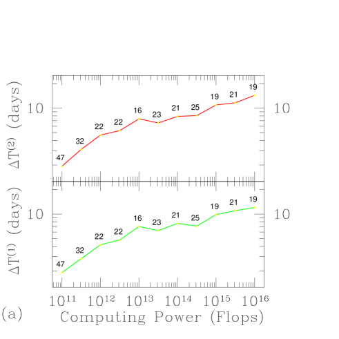
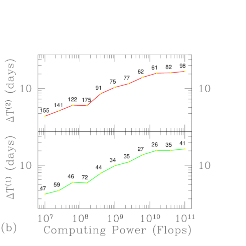
FIG. 9.: The optimum stack length $\Delta T$ (thick solid line) and number of stacks $N$ (numbers along the solid line) for the first and second stages of directed, hierarchical searches. For numerical convenience the maximal projected mismatch was chosen in advance to be $\mu_{\mathrm{max}}=0.3$, and the number of stacks in the first and second stage are the same. The two panels correspond to the following cases: (a) The situation encountered when searching for periodic sources having gravitational wave frequencies up to $1000\mbox{\rm Hz}$, with minimum spindown ages $\tau_{\rm min}=40\mbox{\rm yr}$. (b) The equivalent results for gravitational wave frequencies up to $200\mbox{\rm Hz}$, with minimum spindown ages $\tau_{\rm min}=10^{3}\mbox{\rm yr}$. Both cases assume a threshold which gives an overall statistical significance of $99\%$ to a detection (although the results are insensitive to the precise value).

$$C^{(2)} = \frac{2F^{(1)}N^{(2)}\Delta T^{(2)}N_{pc}^{(2)}}{N_{pf}^{(1)}}\biggl{\{}3f_{\mathrm{max}}[\log_{2}(2f_{\mathrm{max}}\Delta T^{(2)})$$ (51)

$$\ \ +0.5]+\frac{N^{(2)}_{pf}(N^{(2)}-1)}{N^{(2)}N^{(2)}_{pc}\Delta T^{(1)}}\biggr{\}}\;.$$

We require that data analysis proceed at the rate of data acquisition. Since the amount of data used in the second-stage of the search will generally be greater than that used in the first, we require that the analysis be completed in $N^{(2)}\Delta T^{(2)}$ seconds. Thus the computational power is given by

$$P=(C^{(1)}+C^{(2)})/N^{(2)}\Delta T^{(2)}\;.$$ (52)

Our final sensitivity $\Theta$ is given by Eq. (38), using the observation time, mismatch level, and threshold of the second stage of the search. Optimization then consists of maximizing this function over the six parameters $\Delta T^{(1)}$, $\Delta T^{(2)}$, $\mu^{(1)}$, $\mu^{(2)}$, $N^{(1)}$, and $N^{(2)}$, given constraint Eq. (52) for specified $\alpha$, $D$, and $P$.

VI Hierarchical search with stacking

It turns out that the optimization described in the previous section is only weakly sensitive to the parameters $\mu^{(1)}$ and $\mu^{(2)}$; that is, even if we choose values for $\mu^{(1)}$ and $\mu^{(2)}$ quite different from the optimal ones, we can recover nearly all of the sensitivity by adjusting the other parameters for the same computational power $P$. In particular, if we arbitrarily fix $\mu^{(1)}=\mu^{(2)}=0.3$ and re-optimize, we obtain sensitivities within 20% of the optimal.

This becomes very useful when we consider the generalized two-stage hierarchical search with stacking. Normally this would involve optimizing over six variables ($\mu^{(1),(2)}$, $N^{(1),(2)}$, and $\Delta T^{(1),(2)}$) with one constraint on $P$. However, by assuming that we can continue to set $\mu^{(1)}=\mu^{(2)}=0.3$ with minimal loss of sensitivity, we can reduce our degrees of freedom back down to four minus one constraint.

The results of this optimization for our four canonical example searches are given in Figs. 9 and 10. We have again chosen a final confidence level $\alpha=0.99$ and a false dismissal probability of $D=0.01$. Figures 9(a) and (b) show the results for a directed search for old, slow ($\tau_{\mathrm{min}}$=1 000 yr, $f_{\mathrm{max}}$=200 Hz) and young, fast ($\tau_{\mathrm{min}}$=40 yr, $f_{\mathrm{max}}$=1 000 Hz) pulsars, respectively. Figures 10(a) and (b) show the results for an all-sky search for the same two classes of source. The optimal sensitivities achieved by these searches are summarized in Fig. 5(b) in the Introduction.

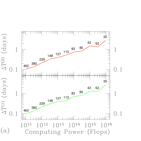
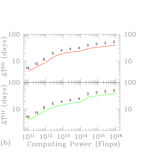
FIG. 10.: Same as in Fig. 9, but for an all-sky search.

VII Specialized searches

The strongest sources of continuous gravitational waves are likely to be the most difficult to detect since the frequency of the waves will be changing significantly as the source radiates angular momentum. As we have seen in the previous sections, an all sky search for these sources is unlikely to achieve the desired sensitivity with available computational resources. To reach better sensitivity levels, it will be useful to consider targeted searches for specific types of source. In this section, we consider three such searches: (i) neutron stars in the galactic core as an example of a limited area sky survey, (ii) newborn neutron stars triggered on optically observed extra-galactic supernovae, and (iii) low mass X-ray binary systems such as Sco X-1.

A Galactic core pulsars

Area surveys of the sky will certainly begin with the region most likely to hold a large number of nearby sources. Based on population models of radio pulsars in our Galaxy [30], there should be many rapidly rotating neutron stars in the galactic bulge. As an example of a limited area search, we therefore consider the optimal strategy for searching an area of 0.004 steradians about the galactic core, for sources with frequencies $f\leq 500$ Hz and spindown ages $\tau\geq 100$ yr. The choice of a 0.004 steradian search is arbitrary; it includes the entire molecular cloud complex at the core of the galaxy ($\sim 300$ pc radius at a distance of $\sim 8.5$ kpc).

It is easy to include a correction factor, to allow for this limited area, in our calculation of the number of patches by reducing the ranges of the integral over $\cal P$ in Eq. (21). Given the approximations in Sec. II B, this amounts to reducing $N_{p}$ in Eq. (29) by

$$0.97\times\left(\frac{0.004}{4\pi}\right)\;,$$ (53)

where the multiplicative factor $0.97$ is the correction for the difference in functional form between the mismatch metric and the angular area metric $d\Omega^{2}=\sin^{2}\theta\,d\theta d\phi$ in the direction of the galactic center (i.e. $-28.9^{\circ}$ declination).

The optimal choices of $N^{(1),(2)}$ and $\Delta T^{(1),(2)}$ for a hierarchical stacked search are shown in Fig. 11 as a function of available computing power; the relative sensitivity of this search is shown in Fig. 6 of the Introduction.

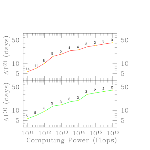
FIG. 11.: The optimum stack length $\Delta T$ (thick solid line) and number of stacks $N$ (numbers along the solid line) for the first and second stages of an hierarchical search for pulsars located in a sky region of $0.004$ steradians about the Galactic center, with $\tau\geq 100$ yr and $f\leq 500$ Hz. For numerical convenience the maximal projected mismatch was chosen in advance to be $\mu_{\mathrm{max}}=0.3$, and the number of stacks in the first and second stage are the same. A threshold is chosen which gives an overall statistical significance of $99\%$ to a detection (although the results are insensitive to the precise value).

We note from Eq. (3.6) of Paper I that gravitational waves from rapidly rotating neutron stars might be expected to have a characteristic amplitude of

$$h_{c}=2.3\times 10^{-25}\frac{\epsilon}{10^{-5}}\frac{I_{zz}}{10^{45}\mathrm{gcm}^{2}}\frac{8.5\mathrm{kpc}}{r}\left(\frac{f}{500\mathrm{Hz}}\right)^{2}\;,$$ (54)

where $\epsilon=(I_{xx}-I_{yy})/I_{zz}$ is the non-axisymmetric strain, $I_{ij}$ is the moment of inertia tensor, $r$ is the distance to the source, $f$ is the gravitational wave frequency, and $h_{c}$ has been averaged over the detector responses to various source inclinations [27]. Theoretical estimates of the strength of the crystalline neutron star crust suggest that it can support static deformations of up to $\epsilon\sim 10^{-5}$, though most neutron stars probably support smaller deformations. From Figs. 3 and 6, we see that 1 Tflops of computing power should allow us to detect pulsars with strains as small as $\epsilon\sim 5\times 10^{-6}$ at $8.5\>\textrm{kpc}$ using enhanced LIGO detectors.

B Newborn neutron stars

Several recent papers [20, 21, 22] have indicated that newly-formed fast-spinning neutron stars may be copious emitters of gravitational radiation. If the newborn neutron star is rotating sufficiently fast, its $r$-modes (axial-vector current oscillations whose restoring force is the Coriolis force) are unstable to gravitational radiation reaction. As the star cools, viscous interactions eventually damp the modes in isolated neutron stars. Numerical studies [23] indicate that neutron stars which are born with rotational frequencies above several hundred Hz will radiate away most of their angular momentum in the form of gravitational waves during their first year of life. Estimates of the viscous time scales, and the superfluid transition temperature, suggest that the $r$-modes are stabilized when the star cools below $\sim 10^{9}$ K and are rotating at $\sim 100$–$200$ Hz. During the evolutionary phase when most of the angular momentum is lost, the amplitude and spindown time scale are expected to be

$$h_{c} = 1.2\times 10^{-24}\sqrt{\kappa}\left(\frac{f}{1\mathrm{kHz}}\right)^{3}\left(\frac{20\mathrm{Mpc}}{r}\right)$$ (55)

$$\tau \approx \frac{580\mathrm{s}}{\kappa}\left(\frac{1\mathrm{kHz}}{f}\right)^{6}\approx{6t}\;.$$ (56)

These estimates are based on Eqs. (4.9) and (5.13) in Ref. [23]. (We note that the “characteristic amplitude” used in Ref. [23] is appropriate to estimate the strength of burst sources, and is different from our $h_{c}$.) Here $\kappa$ is a dimensionless constant of order unity; it parameterizes our ignorance of the non-linear evolution of the $r$-mode instability. The distance to the neutron star is $r$, and $t$ is the actual age of the star. Figure 3 shows $h_{c}$ as a function of frequency with $\kappa=1$ at distances $r=2$ Mpc and $20$ Mpc.

Sources outside our Galaxy are potentially detectable due to the high gravitational-luminosity of a newborn neutron star with an active $r$-mode instability. Nevertheless, it is a significant challenge to develop a feasible search strategy for these signals since the frequency evolves on such short time scales (compared to those considered above). One approach is to perform directed searches on optically observed supernova explosions. Although some supernovae may not be optically visible, and this instability may not operate in all newborn neutron stars, the computational benefits of targeting supernovae are substantial (if not essential). Based on the estimates in Ref. [23], most of the signal to noise is accumulated during the final stages of spindown. With limited computational resources, it seems best to limit the directed searches to frequencies $\lesssim 200$ Hz, when the spindown time scale is $\sim 1$ yr. Figure 12 shows the optimal search criteria in a hierarchical stacked search for neutron stars aged two months or older; the upper frequency cutoff is $f_{\mathrm{max}}=200$ Hz and the minimum spindown timescale is $\tau_{\mathrm{min}}=1$ yr. The sensitivities achievable in a search are shown in Fig. 6 of the Introduction.

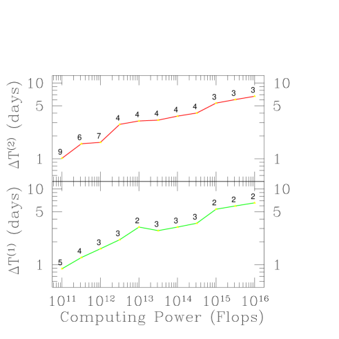
FIG. 12.: The optimum stack length $\Delta T$ (thick solid line) and number of stacks $N$ (numbers along the solid line) for the first and second stages of a hierarchical search for newborn neutron stars spinning down due to an active $r$-mode instability. We assume that a supernova has been identified and accurately located on the sky, so this is a directed search for an object with $\tau_{\mathrm{min}}=1$ yr, and $f\leq 200$ Hz. For numerical convenience the maximal projected mismatch was chosen in advance to be $\mu_{\mathrm{max}}=0.3$, and the number of stacks in the first and second stage are the same. A threshold is chosen which gives an overall statistical significance of $99\%$ to a detection (although the results are insensitive to the precise value).

Figure 6 shows that $1$ Tflops of computing power will not suffice to detect newborn neutron stars as far away as the Virgo cluster ($\approx 20$ Mpc); however, such sources will be marginally detectable within $\sim 8$ Mpc by enhanced LIGO detectors. The NBG catalog [31] lists 165 galaxies within this distance (assuming a Hubble expansion of 75 km/s/Mpc, retarded by the Virgo cluster). From the Hubble types and luminosities of these galaxies, and the supernova event rates in [32], we estimate a total supernova rate of $\sim 0.6$ per year in this volume, of which $\sim 10$% would be of type Ia, $\sim 20$% of type Ib or Ic, and $\sim 70$% of type II. (We note that the total rate is consistent with values given in Ref. [33].) At present, it is not known what fraction of these will produce neutron stars with unstable $r$-modes.

C X-ray binaries

A low-mass x-ray binary (LMXB) is a neutron star orbiting around a stellar companion from which it accretes matter. The accretion process deposits both energy and angular momentum onto the neutron star. The energy is radiated away as x-rays, while the angular momentum spins the star up. Bildsten [24] has suggested that the accretion could create non-axisymmetric temperature gradients in the star, resulting in a substantial mass quadrupole and gravitational wave emission. The star spins up until the gravitational waves are strong enough to radiate away the angular momentum at the same rate as it is accreting; according to Bildsten’s estimates the equilibrium occurs at a gravitational-wave frequency $\sim 500$ Hz. The characteristic gravitational-wave amplitudes from these sources would be

$$h_{c} \gtrsim 4\times 10^{-27}\left(\frac{R}{10\mathrm{km}}\right)^{3/4}\left(\frac{M}{1.4M_{\odot}}\right)^{-1/4}$$ (58)

$$\ \ \times\left(\frac{F}{10^{-8}\mathrm{erg\,cm}^{-2}\mathrm{s}^{-1}}\right)^{1/2}\left(\frac{f}{600\,\mathrm{Hz}}\right)^{-1/2}\;,$$

where $R$ and $M$ are the radius and mass of the neutron star, and $F$ is the observed x-ray flux at the Earth.

The amplitude of the gravitational waves from these sources make them excellent candidates for targeted searches. If the source is an x-ray binary pulsar—an accreting neutron star whose rotation is observable in radio waves—then one can apply the exact phase correction deduced from the radio timing data to optimally detect the gravitational waves. (In this process, one must assume a relationship between the gravitational-wave and radio pulsation frequencies.) Unfortunately, radio pulsations have not been detected from the rapidly rotating neutron stars in all LMXB’s (i.e. neutron stars which rotate hundreds of times a second). In the absence of direct radio observations, estimates of the neutron-star rotation rates are obtained from high-frequency periodic, or quasi-periodic, oscillations in the x-ray output during Type I x-ray bursts. (See Ref. [34] for a summary.) But this does not provide precise timing data for a coherent phase correction. To detect gravitational waves from these sources, one must search over the parameter space of Doppler modulations due to the neutron-star orbit around its companion, and fluctuations in the gravitational-wave frequency due to variable accretion rates. The Doppler effects of the gravitational-wave detector’s motion can be computed exactly, because the sky position of the source is known.

In most cases, the orbital period of an x-ray binary can be deduced from periodicity in its x-ray or optical light curve. In some cases, the radial component of the orbital velocity can be computed by observing an optical emission line from the accretion disk, as was done with the bright x-ray binary Sco X-1 [35]. Such observations do not determine the phase modulation of the gravitational-wave signal with sufficient precision to make the search trivial; however, they do substantially constrain the parameter space of modulations.

In this subsection, we consider a directed search for an x-ray binary in which the orbital parameters are known up to an uncertainty $\delta v$ in the radial velocity $v_{r}$ of the neutron star, and an uncertainty $\delta\phi$ in the orbital phase. It is assumed that long-term photometric observations of the source can give the orbital period $P$ to sufficient precision that we need not search over it explicitly. We therefore parameterize the phase modulations as follows:

$$\phi(t;\mbox{\boldmath${\lambda}$\unboldmath})=2\pi f_{0}\left(t+\frac{v_{1}P}{2\pi c}\cos 2\pi t/P+\frac{v_{2}P}{2\pi c}\sin 2\pi t/P\right)\;,$$ (59)

where $\mbox{\boldmath${\lambda}$\unboldmath}=(f_{0},v_{1},v_{2})$ are our search parameters, the gravitational-wave frequency $f_{0}$ is constrained to be $\leq f_{\mathrm{max}}$, and the pair $(v_{1},v_{2})$ is constrained to lie within an annular arc of radius $v_{r}$, width $\delta v$, and arc angle $\delta\phi$.

Applying the formalism developed in section II to this problem gives essentially the same result as for a sky search over Earth-rotation-induced Doppler modulations if one converts time units by the ratio $P/\mathrm{day}$. In the case of the Earth’s rotation, a search over sky positions $\hat{n}$ corresponds to a search over an area $\pi v_{\mathrm{rot}}^{2}\cos^{2}(\lambda)$ in the equatorial components of the source’s velocity relative to the detector, whereas in the case of a binary orbit, the search is over a coordinate area $v_{r}\delta v\delta\phi$. So we can simply multiply equation (29) by the ratio of these coordinate areas to obtain the number of grid points $N_{p}$ in the parameter space:

$$N_{p} \approx \frac{(f_{\mathrm{max}}P)^{2}}{2\mu_{\mathrm{max}}}\frac{v_{r}\delta v\delta\phi}{c^{2}}\left(A^{-2}+B^{-2}+C^{-2}\right)^{-1/2}\;,$$ (60)

$$A = 0.5\;,$$ (61)

$$B = 1.6(\Delta T/P)^{2}\;,$$ (62)

$$C = 6.4(\Delta T/P)^{5}N^{3}\;.$$ (63)

Accounting for the intrinsic phase variations of the spinning neutron star itself is problematic. Baykal and Ögelman [36] showed empirically that x-ray pulsar frequencies could be well-modeled as a random walk, plus possibly a secular spin up for rapidly-accreting systems. Over a time $t$, the angular rotation rate would undergo excursions up to $\Delta\Omega=\sqrt{St}$, where $S\sim 10^{-17}\mathrm{rad}^{2}\mathrm{s}^{-3}(L_{x}/10^{37}\mathrm{erg\,s}^{-1})$ and $L_{x}$ is the x-ray luminosity of the source. For the sources of interest to us, accretion proceeds at or near the Eddington rate ($L_{x}\sim 3\times 10^{38}$ erg/s), and the gravitational-wave frequency is $f=\Omega/\pi$, so we expect frequency drifts $\sim 2\times 10^{-6}\mathrm{Hz}\sqrt{t/\mathrm{days}}$. If we require that the frequency drifts by less than one Fourier bin $\Delta f\leq 1/t$ during a coherent observation, the observing time $t$ must satisfy

$$t\leq 3.2\>\mathrm{days.}$$ (64)

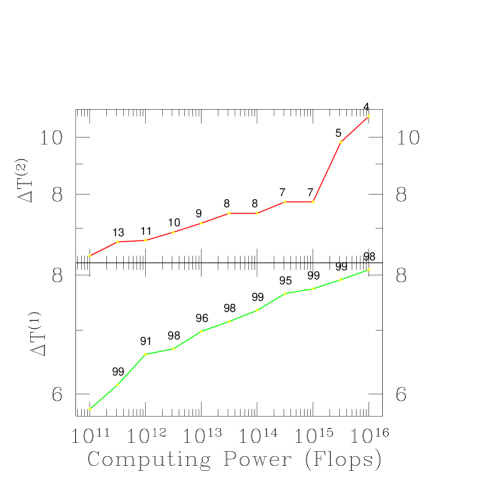
FIG. 13.: The optimum stack length $\Delta T$ (thick solid line) and number of stacks $N$ (numbers along the solid line) for the first and second stages of a hierarchical search for sources of continuous gravitational waves which are in binary systems. We assume the orbit is characterized by two orthogonal velocity parameters which are known to within a total error of $17(\mathrm{km/s})^{2}$, and that the frequency $f\leq 500$ Hz is experiencing a random walk typical of Eddington-rate accretion. For numerical convenience the maximal projected mismatch was chosen in advance to be $\mu_{\mathrm{max}}=0.3$. A threshold is chosen which gives an overall statistical significance of $99\%$ to a detection (although the results are insensitive to the precise value).

This type of random walk cannot be modeled as a low-order polynomial in time. Nevertheless, the stack-slide technique is well suited to search for these sources since corrections for the stochastic changes in frequency can be applied by shifting the stacks by +1, 0, or $-$1 frequency bins when required. In a search using $N$ stacks, each of length $\Delta T$, this kind of correction would be applied after a time $t$ such that

$$2\times 10^{-6}\mathrm{Hz}\sqrt{t/\mathrm{days}}=1/\Delta T\;.$$ (65)

The number of times that these corrections must be applied is then $N\Delta T/t$, and the number of distinct frequency evolutions traced out in this procedure is $3^{N\Delta T/t}$. (Monte-Carlo simulations of stacked FFTs of signals undergoing random walks in frequency have shown that one can increase $t$ by up to a factor of 4, i.e. allowing drifts of up to $\pm 2$ frequency bins, while incurring only $\sim 20\%$ losses in the final summed power.) We have not yet studied in detail how this combines with the mismatches generated from other demodulations, or how to search over all demodulations together in an optimal way. For now we assume a factor of $3^{0.01N(\Delta T/\mathrm{day})^{3}}$ extra points in our search mesh for mismatches of $\mu_{\mathrm{max}}\simeq 0.3$.

As an example, we consider a search for gravitational waves from the neutron star in Sco X-1. This system has an orbital period $P=0.787313\pm 0.000001$ days [37], a radial orbital velocity amplitude of $v_{r}=58.2\pm 3.0$ km/s, an orbital phase known to $\pm 0.10$ radians [35], and an inferred gravitational-wave frequency $f_{\mathrm{max}}\approx 500$ Hz [24]. We note that the uncertainty in $P$ is basically negligible over the $<3.2$ day coherent integrations expected. The remaining uncertainties give:

$$N_{p} = \frac{10^{5}}{\mu_{\mathrm{max}}}3^{0.01N(\Delta T/\mathrm{day})^{3}}\left(A^{-2}+B^{-2}+C^{-2}\right)^{-1/2}\;,$$ (66)

$$A = 0.5\;,$$ (67)

$$B = 2.6(\Delta T/\mathrm{day})^{2}\;,$$ (68)

$$C = 21N^{3}(\Delta T/\mathrm{day})^{5}\;.$$ (69)

where it is understood that $\Delta T\leq 3.2$ days, in order for the random-walk stack-slide corrections to achieve maximum sensitivity.

Figure 13 shows the optimal search criteria for a hierarchical stacked search for the Sco X-1 pulsar under these assumptions. The sensitivities achievable in such a search are shown in Figure 6 of the Introduction. We see that $1$ Tflops of computing power may be sufficient to detect this source using enhanced LIGO detectors if it is radiating most of the accreting angular momentum as gravitational waves. The sensitivity to these sources might be enhanced by a factor $\sim 5$–$10$ if the interferometer is operated in a signal-recycled, narrow-band configuration during the search.

   

VIII Future directions

We have presented in this manuscript the rudiments of a search algorithm for sources of continuous gravitational waves. The next step is to implement some variant of these schemes for a simple test search; a good starting point would be a directed, acceleration (a single spindown parameter) search of a nearby supernova remnant. This will be sufficient to test every stage of the technique, and to assess the accuracy of the computational estimates presented here. It will also allow direct comparison with other approaches such as the line-tracking method that is being explored by Papa [16].

Further theoretical work is required to determine the parameter space which should be searched, especially in the case of active $r$-mode instabilities and radiating neutron stars in LMXB’s. Finally, it would be worthwhile to consider in detail what advantage, if any, can be gained by using data from multiple interferometers at the initial detection stage of a search for continuous gravitational waves.

   

A Patch number formulae

The approximate formulae given in Eqs. (24)–(26) are valid when $N\gg 4$. General expressions for the $G_{s}$ can be derived by setting $\vec{x}=\vec{0}$ in Eqs. (2) and (6), and using Eqs. (11), (16), (17), (18), (20), and (21):

$$G_{1}(N) = \frac{\pi}{6\sqrt{5}}\sqrt{5N^{2}-4}$$ (A1)

$$G_{2}(N) = \frac{\pi^{2}}{180\sqrt{105}}\sqrt{175N^{6}-840N^{4}+1100N^{2}-432}$$ (A2)

$$G_{3}(N) = \frac{\pi^{3}}{75600\sqrt{105}}\sqrt{3675N^{12}-58800N^{10}+363160N^{8}-1053360N^{6}+1484336N^{4}-987840N^{2}+248832}\;.$$ (A3)

In Eq. (21) we approximate the metric as having constant determinant and evaluate it at the point of zero spindown; this introduces small errors of order $(\mbox{[}N\Delta T\mbox{]}/\tau)^{2}$.

Equations (30)–(33) for the number of sky patches ignoring spindown and orbital motions provide an empirical fit to a numerical evaluation of the metric determinant. The determinant was found to have an approximate functional dependence $\sqrt{|\gamma_{ij}|}\sim|\sin 2\theta|$ with corrections of order $v/c\approx 10^{-4}$. Assuming this dependence to be exact, Eqs. (20) and (21) give

$${\cal M}_{s}=\frac{2/\pi}{4\mu_{\mathrm{max}}/(s+2)}\sqrt{\det\left|g_{ij}-\frac{g_{0i}g_{0j}}{g_{00}}\right|_{{}^{f=f_{\mathrm{max}}}_{\theta=\pi/2}}}\;.$$ (A4)

Here $g_{\alpha\beta}$ is the mismatch metric, defined in Eqs. (16)–(18), computed using only the Earth-rotation-induced Doppler modulation. Since the Earth’s rotation is a simple circular motion, and since we are evaluating the metric at a single point in parameter space, we can carry out the integrals in Eq. (18) analytically, to obtain

$$g_{\alpha\beta}=b_{\alpha\beta}-\frac{1}{N}\sum_{k=1}^{N}a_{k\alpha}a_{k\beta}\;,$$ (A5)

where

$$a_{k0} = \left(k-\frac{1}{2}\right)\Delta\Phi+\frac{v/c}{\Delta\Phi}\left\{\sin(k\Delta\Phi)-\sin(\mbox{[}k-1\mbox{]}\Delta\Phi)\right\}$$ (A6)

$$a_{k1} = \frac{f_{\mathrm{max}}v/c}{\Delta\Phi}\left\{\sin(k\Delta\Phi)-\sin(\mbox{[}k-1\mbox{]}\Delta\Phi)\right\}$$ (A7)

$$a_{k2} = \frac{f_{\mathrm{max}}v/c}{\Delta\Phi}\left\{\cos(\mbox{[}k-1\mbox{]}\Delta\Phi)-\cos(k\Delta\Phi)\right\}$$ (A8)

$$b_{00} = \frac{1}{12\Phi}\left\{-24+\frac{v}{c}+6\left(\frac{v}{c}\right)^{2}\Phi+4\Phi^{3}+24\frac{v}{c}\cos\Phi+24\frac{v}{c}\Phi\sin\Phi+3\left(\frac{v}{c}\right)^{2}\sin 2\Phi\right\}$$ (A9)

$$b_{11} = \frac{f_{\mathrm{max}}^{2}(v/c)^{2}}{4\Phi}(2\Phi+\sin 2\Phi)$$ (A10)

$$b_{22} = \frac{f_{\mathrm{max}}^{2}(v/c)^{2}}{4\Phi}(2\Phi-\sin 2\Phi)$$ (A11)

$$b_{01} = b_{10}=\frac{f_{\mathrm{max}}v}{4\Phi}\left\{-4+2\frac{v}{c}\Phi+4\cos\Phi+4\Phi\sin\Phi+\frac{v}{c}\sin 2\Phi\right\}$$ (A12)

$$b_{02} = b_{20}=\frac{f_{\mathrm{max}}v/c}{2\Phi}\left\{-2\Phi\cos\Phi+\sin\Phi\left(2+\frac{v}{c}\sin\Phi\right)\right\}$$ (A13)

$$b_{12} = b_{21}=\frac{f_{\mathrm{max}}^{2}(v/c)^{2}}{2\Phi}\sin^{2}\Phi\;.$$ (A14)

Here $\Phi=2\pi T_{b}/(1\,\mathrm{day})$ is the total angle over which the Earth rotates during the observation, $\Delta\Phi=\Phi/N$ is the angle rotated during each stretch of the data, and $v$ is the maximum radial velocity relative to the detector at latitude $\lambda=45^{\circ}$ of a point at a polar angle $\theta=\pi/4$ on the sky, that is

$$v=\frac{2\pi R_{\mathrm{earth}}\cos\lambda\sin\theta}{1\,\mathrm{day}}\;.$$ (A15)

B Resampling error

In this paper, we have assumed that coherent phase corrections are achieved through stroboscopic resampling: a demodulated time coordinate $t_{b}\mbox{[}t]$ is constructed, and the data stream $h(t)$ is sampled at equal intervals in $t_{b}$ at the Nyquist rate for the highest frequency signal present, $f_{\mathrm{Nyquist}}=2f_{\mathrm{max}}$. However, since the data stream is initially sampled at some finite rate $f_{s}=Rf_{\mathrm{Nyquist}}$ (where $R$ is the oversampling factor), this can introduce errors: in general, there will not be a data point exactly at a given value of $t_{b}$, so the nearest (in time) datum must be substituted. Consequently, there will be residual phase errors $\Delta\Phi(t)\in[-\pi/2R,\pi/2R)$ caused by rounding to the nearest datum even if one chooses a phase model whose frequency and modulation parameters exactly match the signal. The phase of the resampled signal drifts until the timing error is $\geq 1/2f_{s}$, at which point one corrects the phase by sampling an adjacent datum, which shifts in time by $1/f_{s}$. These residual phase errors reduce the Fourier amplitude of the signal by a fraction

$$F=\left|\frac{1}{N}\sum_{k=1}^{N}e^{i\Delta\Phi(k/f_{\mathrm{Nyquist}})}\right|\;,$$ (B1)

where $N=f_{\mathrm{Nyquist}}\Delta T$ is the total number of points in the resampled data stream.

The uncorrected signal will in general drift by many radians in phase, which is the reason why we must apply phase corrections in the first place. This means that $\Delta\Phi(t)$ will sweep through the range $[-\pi/2R,\pi/2R)$ many times over the course of the observation. So, regardless of the precise form of the phase evolution, we expect $\Delta\Phi(k/f_{\mathrm{Nyquist}})$ to be essentially evenly distributed over this interval. Thus, replacing the sum with an expectation integral, we have

$$F\approx\left|\frac{R}{\pi}\int_{-\pi/2R}^{\pi/2R}e^{i\Phi}\,d\Phi\right|=\frac{\sin(\pi/2R)}{\pi/2R}\;.$$ (B2)

The fractional losses in amplitude $1-F$ for a few values of the oversampling factor $R$ are given in Table I.

TABLE I.: The percentage reduction $(1-F)$ in amplitude of a signal as a function of the oversampling factor $R$. The LIGO interferometers will collect data at $f_{s}=16\;384$Hz, so that the data will be oversampled by $R\geq 4$ compared to the maximum gravitational wave frequency that we expect on physical grounds. In fact, it seems more likely that $R\simeq 8$ for real signals.

$R$=	2	3	4	5	6	7	8
$1-F$=	10.0%	4.5%	2.6%	1.6%	1.1%	0.8%	0.6%

The highest gravitational-wave frequencies we consider are 1000 Hz, requiring a resampling rate of $f_{\mathrm{Nyquist}}=2000$ Hz. Since LIGO will acquire data at a rate of $16\;384$Hz, corresponding to an oversampling factor of $R>8$, we have a maximum signal loss due to resampling of $1-F=0.6\%$. Resampling errors will increase if the number of data samples is reduced by some factor before phase-correcting.

REFERENCES

- [1] P. R. Brady, T. Creighton, C. Cutler, and B. F. Schutz, Phys. Rev. D57, 2101 (1998).
- [2] J. C. Livas, Ph.D. thesis, Massachusetts Institute of Technology, 1987.
- [3] G. S. Jones, Ph.D. thesis, University of Whales, 1995.
- [4] T. M. Niebauer et al., Phys. Rev. D 47, 3106 (1993).
- [5] S. Chandrasekhar, Phys. Rev. Let. 24, 611 (1970).
- [6] J. L. Friedman and B. F. Schutz, Ap. J. 222, 281 (1978).
- [7] S. Bonazzola and E. Gourgoulhon, Astron. Astr. 312, 675 (1996).
- [8] M. Zimmermann, Phys. Rev. D. 21, 891 (1980).
- [9] M. Zimmermann and E. Szedenits, Jr., Phys. Rev. D. 20, 351 (1979).
- [10] R. V. Wagoner, Astrophys. J. 278, 345 (1984).
- [11] D. V. Gal’tsov, V. P. Tsvetkov, and A. N. Tsirulev, Sov. Phys. —JETP 59, 472 (1984).
- [12] K. C. B. New, G. Chanmugam, W. W. Johnson, and J. E. Tohline, Ap. J. 450, 757 (1995).
- [13] A. Krolak, Searching data for periodic signals, gr-qc/9803055.
- [14] P. Jaranowski, A. Krolak, and B. F. Schutz, Phys. Rev. D58, 063001 (1998), gr-qc/9804014.
- [15] P. Jaranowski and A. Krolak, Data analysis of gravitational wave signals from spinning neutron stars. 2. Accuracy of estimation of parameters, gr-qc/9809046.
- [16] M. A. Papa, B. F. Schutz, S. Frasca and P. Astone, Detection of continuous gravitational wave signals: pattern tracking with the Hough transform, to appear in Proceedings of the LISA Symposium (1998); M.A. Papa, P. Astone, S.Frasca and B.F. Schutz, Searching for continuous waves by line identification, to appear in the proceedings of Gravitational Wave Data Analysis Workshop (1997); M. A. Papa, private communication.
- [17] S. L. Shapiro, S. A. Teukolsky, and I. Wasserman, Ap. J. 272, 702 (1984).
- [18] J. L. Friedman, J. R. Ipser, and L. Parker, Nature 312, 255 (1984).
- [19] S. R. Kulkarni, Phil. Trans. R. Soc. Lond. A 341, 77 (1992).
- [20] N. Andersson, Astrophys. J. 502, 708 (1998), gr-qc/9706075.
- [21] J. L. Friedman and S. M. Morsink, Astrophys. J. 502, 714 (1998), gr-qc/9706073.
- [22] L. Lindblom, B. J. Owen, and S. M. Morsink, Phys. Rev. Lett. 80, 4843 (1998).
- [23] B. J. Owen et al., Phys. Rev. D58, 084020 (1998), gr-qc/9804044.
- [24] L. Bildsten, Astrophys. J. 501, L89 1998, astro-ph/9804325.
- [25] B. F. Schutz, in The Detection of Gravitational Waves, edited by D. G. Blair (Cambridge University Press, Cambridge, 1991), Chap. 16, pp. 406–451.
- [26] The method of stacking power-spectra has been used by radio astronomers in deep searches for millisecond pulsars, although all coreections were applied to the data stream via resampling and not sliding the spectra. For more information on the implementation, see S. B. Anderson, Ph.D. thesis, California Institute of Technology, 1993.
- [27] K. S. Thorne, in Three hundred years of gravitation, edited by S. W. Hawking and W. Israel (Cambridge University Press, Cambridge, 1987), Chap. 9, pp. 330–458.
- [28] B. F. Schutz, Sources of radiation from neutron stars, gr-qc/9802020; and, talk given at Gravitational Wave Data Analysis Workshop, MIT (1996).
- [29] B. Owen, Phys. Rev. D. 53, 6749 (1996).
- [30] S. J. Curran and D. R. Lorimer, Mon. Not. R. Astron. Soc. 276, 347 (1995).
- [31] R. B. Tully, Nearby Galaxy Catalog (Cambridge University Press, Cambridge, 1988).
- [32] S. van den Bergh and R. D. McClure, Ap. J. 425, 205 (1994).
- [33] R. Talbot, Ap. J. 205, 535 (1976).
- [34] M. van der Klis, in The Many Faces of Neutron Stars, edited by A. Alpar, L. Buccheri, and J. van Paradijs (Kluwer, Dordrecht, 1998 (in press)).
- [35] A. P. Cowley and D. Crampton, Ap. J. Letters 201, L65 (1975).
- [36] A. Baykal and H. Ögelman, Astron. Astrophys. 267, 119 (1993).
- [37] E. W. Gottlieb, E. L. Wright, and W. Liller, Ap. J. Letters 195, L33 (1975).