Geodesic Deviation in Regge Calculus

Abstract

Geodesic deviation is the most basic manifestation of the influence of gravitational fields on matter. We investigate geodesic deviation within the framework of Regge calculus, and compare the results with the continuous formulation of general relativity on two different levels. We show that the continuum and simplicial descriptions coincide when the cumulative effect of the Regge contributions over an infinitesimal element of area is considered. This comparison provides a quantitative relation between the curvature of the continuous description and the deficit angles of Regge calculus. The results presented might also be of help in developing generic ways of including matter terms in the Regge equations.

1 Introduction

A generic description of the interaction between gravitational fields and matter is an open question in the Regge formulation of general relativity [1, 2, 3]. There has been some progress towards the inclusion of matter terms in the Regge formulation (cf., for instance, Dubal [4]), but this has come at the price of restrictions on the kind of matter which can be coupled to the gravitational field, together with restrictions on the symmetries of the field.

A possible approach to a more general description of matter in Regge calculus is to capitalize on our experience with the standard continuous formulation of general relativity. If there was a dependable way of identifying the parameters describing matter in both descriptions one could simply insert appropriate terms in the Regge equations, based on expressions for the energy–momentum which enters the right hand side of Einstein’s equations.

Unfortunately, such an identification is non-trivial, and straightforward attempts on the level of a single cell (defined as the collection of simplices attached to a single hinge in the lattice) typically leads to divergence in the continuum limit. This is caused by the need to compare the nonlocalizable parameters of Regge calculus to continuum quantities localized at points, such as the energy–momentum tensor. For some particular cases, the continuum theory can be described using parameters which are definable within the Regge description [4]. These results, however exciting, do not seem able to provide methods that are applicable in more generic settings.

A better understanding of the relation between the parameters of Regge calculus and those of the continuum description might provide some ground for progress in this direction. In this paper, we analyze the most basic and elementary manifestation of the influence of gravity on matter, namely, geodesic deviation.

In Section 2 we briefly describe geodesic deviation in the continuum formulation, mainly to establish the notations and restrictions to be used in subsequent sections of the paper. In Section 3 we introduce and discuss geodesic deviation in Regge calculus. Section 4 compares the Regge formulation of geodesic deviation with the continuum description, which results in a relation between the Riemann curvature of the continuum and the deficit angles of Regge calculus. Finally, in section 5, we show briefly how our results extend almost trivially to a four-dimensional simplicial lattice.

2 Geodesic Deviation in the Continuum

Geodesic deviation represents the simplest and most basic manifestation of the influence of the gravitational field on matter. It describes the relative acceleration of free test particles (the contribution of these particles as sources of gravity is neglected) caused by spacetime curvature. As such, it is described in full in practically any modern text on general relativity (cf., for instance Misner, Thorne and Wheeler [2], or Synge [5]). In what follows we use notations similar to those of Synge [5], since they resemble more closely the expressions we will obtain from the analysis of geodesic deviation in Regge calculus.

Figure 1: A one parameter family of geodesics is used to illustrate geodesic deviation in the continuum. Each geodesic is identified by a unique label $v$, with the position along each geodesic parameterized by $u$. The vectors ${\mathbf{u}}$ and ${\mathbf{v}}$ are tangent to the $v$=constant and $u$=constant lines, respectively. The infinitesimal separation vector between geodesics is $\Delta v\,\partial_{v}$.

The deviation of nearby geodesics is usually described by considering a congruence of curves $C(v)$ parametrized by $v$ in such a way that $v={\rm const}$ along each curve, with each of these curves parametrized by $u$. Within a coordinate patch, the whole congruence is given by the equations $x^{\mu}=x^{\mu}(u,v)$, as indicated in figure 1. The curves of the congruence mesh to form a 2–surface. That is, the vectors

$${\mathbf{u}}=\partial_{u}={\partial\over\partial u}$$ (1)

which is tangent to the $u$–lines (the constituent lines of the congruence), and

$${\mathbf{v}}=\partial_{v}={\partial\over\partial v},$$ (2)

which is tangent to $v$–lines, commute

$${\delta\over\delta v}\left({\partial\over\partial u}\right)={\delta\over\delta u}\left({\partial\over\partial v}\right).$$ (3)

Here $\delta/\delta u$ and $\delta/\delta v$ are the covariant derivatives along $u$– and $v$–lines of the congruence.

In studying a pair of adjacent curves $C(v)$ and $C(v+\Delta v)$ one deals with the infinitesimal separation vector

$${\mathbf{V}}=\Delta v\,{\partial\over\partial v}.$$ (4)

Our aim is to find how $C(v+\Delta v)$ deviates from $C(v)$. One writes down the equation for the second covariant derivative of the the separation vector ${\mathbf{V}}$, along the curve $C(v)$ parametrized by $u$.

We are interested in the situation when the curves $C(v)$ are geodesics parametrized by an affine parameter $u$,

$${\delta{\mathbf{u}}\over\delta u}=0,$$ (5)

in which case the equation for the separation vector, called the geodesic deviation equation, takes the form

$${\delta^{2}{\mathbf{V}}\over\delta u^{2}}+{\mathbf{R}}({\mathbf{u}},{\mathbf{V}},{\mathbf{u}})=0.$$ (6)

In a coordinate frame on the patch of spacetime the equation reads

$${\delta^{2}V^{\mu}\over\delta u^{2}}+{R^{\mu}}_{\lambda\nu\kappa}\,u^{\lambda}V^{\nu}u^{\kappa}=0.$$ (7)

In subsequent sections we will mainly have in mind the case when the lines $C(v)$ are either timelike or spacelike, with the parameter $u$ picked to be the arc length parameter $s$, and the $v$–lines orthogonal to the $u$–lines (the lines $C(v)$ of the congruence). The geodesic deviation equation then takes form

$${\delta^{2}{\mathbf{V}}\over\delta s^{2}}+{\mathbf{R}}({\mathbf{u}},{\mathbf{V}},{\mathbf{u}})=0,$$ (8)

and the tangent $u$–vector ${\mathbf{u}}$ becomes a unit vector (the 4–velocity vector, if the curves $C(v)$ are timelike).

In addition, as we shall see, the key feature of our investigation shows up clearly for spacetimes of dimension two. We shall therefore restrict ourselves to this case, as the exposition in higher dimensions only clouds the basic issues. In two dimensions the Riemann tensor has only one nonzero component, which we take to be $R^{1}_{\ 212}$ (cf. Section 4).

3 Geodesic Deviation in Regge Calculus

In this section we discuss the most elementary aspects of geodesic deviation in Regge calculus. We choose the pictorial representation shown in figure 2 to summarize the conclusions important for our purpose.

It is sufficient to consider the case of a two–dimensional spacetime, where the curvature is concentrated entirely at the vertices of the simplicial lattice. At any particular vertex it is usually pictured as the deficit angle [2], which emerges if one attempts to map isometrically the neighborhood of the vertex (consisting of all triangles emanating from the vertex) to the plane. Such a map involves cutting the neighborhood along one or more edges coming from the vertex and spreading it on the plane.

Figure 2 shows two initially parallel geodesics pass on different sides of a single vertex. The geodesics are seen to converge (or diverge) due to the curvature concentrated at the vertex. Each geodesic is represented by a straight line. More precisely, the geodesic is described as being a straight line within each triangle, and does not change direction when intersecting the boundary of the triangle. The value and meaning of this more precise description becomes clear when one realizes that the pictorial representation of geodesic deviation presented in figure 2 is not unique.

Figure 3(a) shows an alternative pictorial representation, where each geodesic consists of pieces of a straight line. The deficit angle at the vertex is represented as the sum of the deficit angles associated with each cut. Figure’s 2(b) and 3(a) both provide truthful representations of geodesic deviation around a single vertex.

(a)                                                      (b)

Figure 2: (a) Two originally parallel test-particle world lines (dotted lines), are seen to converge as they enter the triangle $(023)$. The curvature that brings them together after the fashion of gravity on this two dimensional manifold is concentrated on the vertex (or “hinge”) $0$, where the four triangles meet. (b) A pictorial representation of the deficit angle $\epsilon$ at the vertex $0$. By embedding the lattice in three-dimensions, making a cut along one edge, and flattening the resulting structure onto a plane, the deficit angle at the vertex becomes apparent. In this picture, the geodesics are straight lines within each triangle, and do not change direction as they pass from one triangle to the next. The deviation of initially parallel geodesics only becomes apparent when the geodesics are compared within triangle $(023)$.

Another picture of geodesic deviation, which appears more reminiscent of the continuum picture, can be obtained if one uses a non–isometric map to represent the neighborhood of a vertex. For instance, one can follow Friedberg and Lee [6] and embed the neighborhood of the vertex in a 3–dimensional space, and then project it onto a plane (this representation is not unique, as was the case with isometric maps). There is no deficit angle under such a mapping. The information about curvature is contained in the metric that changes from one triangle projection to another (but remains constant within each triangle). The geodesic deviation in this representation is pictured in figure 3(b). Each geodesic is represented by a piecewise straight line. It is straight within each triangle but experiences refractions at the edges of a triangle (due to jumps in the metric, and resulting pulses in the connection coefficients). For a more detailed description in a general setting, see Williams and Ellis [7, 8].

This new picture is equivalent to that presented in figure 3(a), the only difference being the frame used for describing geodesic deviation. Figure 3(b) uses a holonomic frame, where all information about the curvature resides in the metric, which changes from one triangular patch to the next. Figure 3(a) uses a nonholonomic frame with a constant metric, where all information about curvature is in the nonholonomicity object, thus generating pulses in the connection co-efficients when crossing from one triangle to the next.

Both representations lead to a very simple description of covariant differentiation. In the standard representation, figure 3(a), within each triangle we use the frame determined by the edges emanating from a vertex, and assume that the metric is globally flat. Covariant derivatives inside each triangle then coincide with partial derivatives. When passing from one triangle to another we perform only a transformation of the frame.

In the alternate description, figure 3(b), the coordinate system is common for all triangles, but the metric is flat only within each triangle, varying from one triangle to another in a jump. The covariant derivative looks almost the same as in the standard description, except that the jumps on the triangular joints are caused by jumps in the metric.

(a)	(b)

Figure 3: Two other possible representations of the deficit angle about the central vertex. (a) A cut is made along each edge meeting at the vertex, and the deficit is partitioned among all such edges. Geodesics are now straight lines within each triangle, with pulses in the connection co-efficients at each triangular boundary. (b) A non-isometric mapping, which yields a flat metric inside each triangle. The co-ordinate system is common to all triangles in the patch, and the metric jumps when one moves from one triangle to the next. This introduces refractions in the geodesic paths.

Whatever description of geodesic deviation one chooses, for geodesics going around one isolated vertex the curvature manifests itself in a change of the angle of convergence of the geodesics, $\Delta\alpha$. The total change in the angle between two such geodesics is equal to the deficit angle $\epsilon$ associated with the vertex,

$$\Delta\alpha=\epsilon.$$ (9)

Just as in the continuum case, the curvature focuses (or scatters) geodesics.

(a)                                                      (b)

Figure 4: The discontinuity in the deflection angle for intially parallel test particles as a function of the separation makes it impossible to define, in a straighforward way, the Regge calculus analog of geodesic deviation for an isolated vertex. (a) A collection of initially parallel worldlines. Two paths which pass around the same side of the vertex do not experience geodesic deviation. (b) As a function of the separation between the worldlines, the deviation angle shows sharp jumps.

This is where the similarity ends. There can be no continuous change in $\Delta\alpha$ for a one parametric family of geodesics. That is, geodesics on one side of the vertex remain parallel — see figure 4. There is no possibility of introducing, in a straight-forward way, anything similar to the geodesic deviation equation of the continuum, which depends on the second derivative of the separation vector.

We are not aware of a prescription for comparing the measure of spacetime curvature in Regge calculus with that of the continuum on this level. Any attempt to localize curvature in this way at a single vertex yields an inherently divergent procedure in the continuum limit, which is not surprising.

4 Comparison with the Continuum: A Regge Interpretation of Geodesic Deviation.

A comparison of geodesic deviation in Regge calculus with the standard continuum description can be achieved by deriving the geodesic deviation equation in terms of the curvature descriptors (deficit angles) of Regge calculus, and comparing the result with the continuum geodesic deviation equation (8). This comparison should provide a relation between the representation of curvature in Regge calculus – the deficit angles – and the Riemannian curvature of the continuum.

In order to achieve our goal, we consider a domain of the Regge lattice containing $N$ vertices with deficit angles ${\{\epsilon_{i}\}}_{i=1}^{N}$ (cf. figure  5(a)). We assume that each deficit angle $\epsilon_{i}$ is small, as is the area $\Delta A$ containing the vertices, but the total deficit angle per unit area

$$\Theta=\frac{1}{\Delta A}\,{\sum_{i=1}^{N}}\epsilon_{i}=n\overline{\epsilon}$$ (10)

is finite. The symbol $n$ in equation (10) represents the density of vertices per unit area, and $\overline{\epsilon}$ is the average deficit angle per vertex, defined as

$$\overline{\epsilon}=\frac{1}{N}\,{\sum_{i=1}^{N}\epsilon_{i}}.$$ (11)

The precise measure of the area is unimportant at this stage, and will be provided later. It is important to note, however, that the total deficit $\sum_{i=1}^{N}\epsilon_{i}$ is small, too.

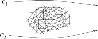
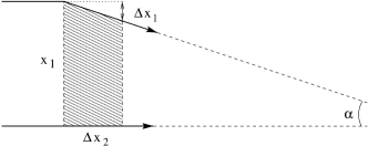
(a)	(b)

Figure 5: (a) Geodesics $C_{1}$ and $C_{2}$ enclose a region containing $N$ vertices. (b) One possible representation of the geodesic deviation induced in two initially parallel test particles as they pass a region containing $N$ vertices.

Let us consider the portion of the congruence of geodesics between the geodesics $C_{1}$ and $C_{2}$ that contains these $N$ vertices, and no others. It is clear that the change in the convergence angle between these two geodesics after passing around the area is determined by the total deficit angle attributed to the area,

$$\Delta\alpha=\sum_{i=1}^{N}\epsilon_{i}.$$ (12)

We assume now that each geodesic of the congruence is parametrized by the arc length parameter $s$, and that the curves of the congruence are labeled by another parameter $v$ in such a way that the lines $s={\rm const}$ are orthogonal to geodesics. Let us approximate the whole picture by a piece of differentiable manifold with its curvature determined by the Riemannian tensor ${\mathbf{R}}$, which has only one component in two dimensions. Introduce on this manifold coordinates $(x^{1},x^{2})$ in such a way that the $x^{1}$–coordinate lines satisfy $v={\rm const}$, while $x^{2}$–coordinate lines follow the geodesics of the congruence.

The image of the domain between the geodesics, which contains the $N$ vertices, determines an infinitesimal rectangle $x^{1}$ by $\Delta x^{2}$ with area $\Delta A=x^{1}\,\Delta x^{2}$. The components of the separation vector ${\mathbf{V}}$ and the 4–velocity vector ${\mathbf{u}}$ are given by

$${\mathbf{V}}=\langle x^{1},0\rangle$$ (13)

and

$${\mathbf{u}}=\left\langle 0,{\Delta x^{2}\over\Delta s}\right\rangle=\langle 0,1\rangle,$$ (14)

where the “size” of the separation vector ${\mathbf{V}}$ is equal to $x^{1}$. It can be seen from figure 5(b) that the (small) convergence angle $\alpha$ is expressed in terms of $\Delta x^{1},\Delta x^{2}$ as

$$\alpha=-{\Delta x^{1}\over\Delta x^{2}}.$$ (15)

With this in mind, equation (12) can be rewritten as

$$-\Delta\left({\Delta x^{1}\over\Delta x^{2}}\right)=\sum_{i=1}^{N}\epsilon_{i}=n\overline{\epsilon}\,\Delta A=n\overline{\epsilon}\,x^{1}\Delta x^{2},$$ (16)

and taking into account that $\Delta x^{2}=\Delta s$, this implies

$${\Delta\over\Delta s}\left({\Delta V\over\Delta s}\right)+n\overline{\epsilon}\,V=0$$ (17)

where $V$ is just another notation for the “size” of the separation vector.

The infinitesimal version of the last equation (cf. remarks concerning the covariant derivatives on the Regge lattice) yields the equation for the first component of the separation vector ${\mathbf{V}}=\langle V^{1},0\rangle$, namely

$${\delta^{2}V^{1}\over\delta s^{2}}+n\overline{\epsilon}\,V^{1}=0.$$ (18)

The continuum geodesic deviation equation (8), when applied to the configuration shown in figure 5, yields

$${\delta^{2}V^{1}\over\delta s^{2}}+{R^{1}}_{212}\,V^{1}=0,$$

for the first component of the separation vector. Comparison of this continuum expression with equation (18) clearly demonstrates that not only has the geodesic deviation equation of the continuum been recovered, but the interpretation of the Riemannian curvature in terms of the simplicial deficit angles has been obtained as well. That is,

$${R^{1}}_{212}=n\overline{\epsilon},$$ (19)

and hence the single component of the Riemann curvature tensor may be interpreted as the average deficit angle per unit area.

5 The transition to four dimensions

We now consider the generalization of the previous results to four dimensions. It is important to note that the fundamental nature of the problem does not change as we make the transition to a four dimensional lattice. In the Regge description, the curvature in four-dimensions is concentrated on the triangular hinges of the lattice. In the continuum, the four dimensional Riemann curvature tensor has twenty independent components.

Consider again the situation depicted in figure 5, only now imagine that the infinitesimal region contains $N$ triangular hinges with associated deficit angles $\{\epsilon_{i}\}_{i=1}^{N}$. For a test particle which lies in the plane orthogonal to one such hinge, the tangent vector undergoes a rotation equal to the magnitude of the deficit angle concentrated on the hinge. This is identical to the two dimensional case.

In general, our test particles do not lie on a plane orthogonal to the hinges, and indeed, the hinges themselves have no overall orientation. If we consider a vector that initially makes an angle $\theta$ with the plane orthogonal to a single hinge, then the component of the vector which lies in the plane will undergo a rotation equal to the deficit angle. This implies that the tangent vector itself undergoes a rotation of $\epsilon\cos\theta$.

Let us again consider the congruence of geodesics between $C_{1}$ and $C_{2}$, which encloses the region containing $N$ hinges. Let ${\mathbf{u}}$ be tangent to a geodesic in this congruence. We define the average effective deficit angle experienced by this geodesic to be

$$\overline{\epsilon}_{\mathbf{u}}=\frac{1}{N}\sum_{i=1}^{N}\epsilon_{i}\cos\theta_{i},$$ (20)

where $\theta_{i}$ is the initial angle between the tangent vector ${\mathbf{u}}$ and the plane orthogonal to the hinge $\epsilon_{i}$.

It is now clear how all components of the four-dimensional Riemann tensor may be calculated in the continuum limit. Given two initially parallel geodesics, the calculations of section 4 are applied, with the average deficit $\overline{\epsilon}$ everywhere replaced with the average effective deficit in that direction, $\overline{\epsilon}_{\mathbf{u}}$. The density of hinges per unit area, $n$, is replaced with the density of hinges per unit volume. Repeating this calculation with various choices of ${\mathbf{u}}$ will yield all components of the Riemann tensor. We see that in four dimensions, the Riemann tensor may be viewed as the average effective deficit angle per unit volume.

6 Conclusion

We have considered geodesic deviation in Regge calculus. On the level of an elementary cell the similarity between the Regge and continuum descriptions is rather tenuous, reduced only to the focusing (or scattering) of geodesics. Attempts to localize the description of geodesic deviation on this level result in a divergent procedure.

The situation considerably improves when we compute the cumulative effect of the vertices contained in an infinitesimal element of area (infinitesimal in the context of the continuum description). In fact, by considering this region we reproduce the geodesic deviation equation of the continuum, and, in doing so, obtain an interpretation of the Riemannian curvature of spacetime as the effective deficit angle per unit volume. The localization procedure (infinitesimal by the continuum standard) becomes convergent in the continuum limit, and the cause of the divergences on the level of one cell becomes, in an obvious way, responsible for the errors of the approximation. These may, in principle, be reduced to desirable values.

References

References

- [1] T. Regge, Nuovo Cimento, 19, 558 (1961).
- [2] C. W. Misner, K. S. Thorne and J.A. Wheeler, Gravitation, W.H. Freeman, San Francisco, 1973.
- [3] R. M. Williams and P. A. Tuckey, Class. Quantum Grav., 9, 1409–22 (1992).
- [4] M. R. Dubal, Class. Quantum Grav., 6, 1925–41 (1989).
- [5] J. L. Synge, Relativity: the General Theory, North-Holland Publishing Co., Amsterdam, 1966.
- [6] R. Friedberg and T. D. Lee, Nucl. Phys., B242, 145–66 (1984).
- [7] R. M. Williams and G. F. R. Ellis, Gen. Rel. Grav., 13, 361–95 (1981).
- [8] R. M. Williams and G. F. R. Ellis, Gen. Rel. Grav., 16, 1003–21 (1984).