We study solutions of the Wheeler-DeWitt equation corresponding to an $S$-modular invariant ${\cal N}=1$ supergravity model and a closed homogeneous and isotropic Friedmann-Robertson-Walker spacetime. The issues of inflation and the cosmological constant problem are addressed with the help of the relevant wave functions. We find that topological type inflation is consistent from the quantum mechanical point of view and that a solution for the cosmological constant problem along the lines of the strong CP problem naturally arises.

1 Introduction

Duality symmetries play a fundamental role in modern string theories. These symmetries made it possible to understand that all five known string theories, as well as eleven-dimensional supergravity, are the weakly coupled limit of a single and more comprehensive structure named $M$-Theory. The basic dualities are of two types and are referred to as $T$-dualities and $S$-dualities. Moreover, these dualities are combined in a more general symmetry, called $U$-duality. These transformations relate different, however equivalent, string theories [1]. The first example encountered of such a symmetry, named target space modular invariance or $T$-duality, was the $O(d,d)$ transformation connecting all toroidal compactifications in $d$-dimensions [2]. In this case, it was shown that the duality symmetry holds to all orders in the string loop expansion parameter, through a suitable change in the dilaton when transforming both metric and torsion fields [3]. Furthermore, it was shown that the effective supergravity action following from string compactifications on orbifolds or Calabi-Yau manifolds is constrained by an underlying string symmetry, the mentioned target space modular invariance. The target space modular group $PSL(2,{\bf Z})$ acts on the complex scalar field T as

$$T\to\frac{aT-ib}{icT+d};\qquad a,b,c,d\in{\bf Z},\quad ad-bc=1,$$ (1)

where $\langle T\rangle$ is the background modulus associated to the overall scale of the internal six-dimensional space on which the string theory is compactified, $T=R^{2}+iB$, with $R$ being the “radius” of the internal space and $B$ an internal axion. The target space modular transformation contains the well-known duality transformation $R\to 1/R$, as well as discrete shifts of the axionic background $B$, and it was shown that this symmetry remains unbroken at any order in string perturbation theory.

An important subset of these duality symmetries is the so-called scale-factor or Abelian duality of string models embedded in flat homogeneous and isotropic spacetimes [4]. The scale-factor duality symmetry is present in the lowest order string effective action, implying that the transformation of the scale factor of a homogeneous and isotropic target space metric, $a(t)\to\pm a^{-1}(t)$, would leave the model invariant provided that, in $d$ spatial dimensions, the string coupling – the dilaton $\phi$ – is transformed as

$$\phi(t)\rightarrow\phi(t)-{d\over 2}\ln a(t)~{}.$$ (2)

Other transformations were also proposed to implement these dualities for backgrounds with non-Abelian isometry groups which are, in principle, compatible with homogeneous Bianchi cosmological backgrounds [5].

Already at the classical level, string theory allows for cosmological models with scale-factor duality symmetry from which important issues such as the problem of the initial singularity, inflation and the generation of primordial density fluctuations and gravitational waves can be addressed. Scale-factor duality leads also to interesting cosmological scenarios as, for instance, the Pre-Big-Bang [6] (see [7] and references therein for an updated account) which assumes the Universe has undergone a period of accelerated contraction towards the Big-Bang singularity and emerged due to yet unknown stringy effects in the expanding standard radiation dominated Friedmann-Robertson-Walker phase. This contracting phase has presumably been driven by the dilaton kinetic energy and would give origin to a substantial amount of gravitational waves which would then be a distinct observational signature of this scenario. Nevertheless, despite its appealing features, the Pre-Big-Bang scenario is plagued, at least in its simplest versions, with serious inconsistencies such as fine-tuning and instabilities that invalidate the tree level picture [8] and also with the lacking of a mechanism ensuring the transition from the Pre-Big-Bang phase towards the standard hot Big-Bang model [9]. Actually, obtaining a period of inflation that emerges naturally from string theory is known to be a notoriously hard problem and many suggestions have been proposed [10, 11, 12, 13]. We shall discuss in this paper a proposal in the context of dual ${\cal N}=1$ supergravity that is based on the idea of topological inflation and see how quantum cosmology does actually support some of its assumptions. Anyway, independently from the above mentioned difficulties, it is possible to show, for instance, that string cosmological models where the scale-factor duality symmetry holds naturally allow for an evolution towards a radiation-dominated phase [14]. Of course, a consistent treatment of issues related with the very early Universe requires understanding of the higher curvature regime, where quantum gravity effects are important, and the question of whether string symmetries still hold in the quantized version of the theory is quite relevant. As a complete quantum field theory of closed strings is notoriously difficult to handle, one hopes to get some insight into the full theory by considering the quantum cosmology of the low-energy effective action (for a discussion on the validity and consistency of the effective action procedure in quantum cosmology see, for instance, Ref. [15]). The issue of whether scale-factor duality survives at the quantum level, was considered via the canonical quantization of the lowest order string effective action using the standard ADM formalism in an ${\bf R}\times S^{3}$ topology in Ref. [16]. There, it was shown within the formalism of quantum cosmology and its interpretative framework [17] that, although scale-factor duality is lost as an exact symmetry of the resulting minisuperspace model, it still holds as an approximate symmetry of the classical string model, as the wave function was shown to peak for field configurations consistent with this symmetry. The analysis of the one-loop string effective models which exhibit the full $O(d,d)$ symmetry was studied in Ref. [18]. Furthermore, the quantum treatment has also been considered to address the question of whether a quantum transition would allow for an exit from the Pre-Big-Bang phase to the standard radiation dominated phase [19]. We mention in relation to these issues, that the conditions under which quantum cosmology based on the low-energy Einstein-Hilbert action arises from a subgroup of the modular group of $M$-theory, as well as how duality transformations can resolve apparent cosmological singularities has been recently discussed in Ref. [20].

$S$-duality was conjectured [21] in analogy with $T$-duality. This conjectured symmetry would be a further modular invariance in the resulting ${\cal N}=1$ supergravity model arising from string theory, where the modular group acts on the complex scalar field (which is the lowest order component of a chiral superfield in the 4-dimensional string), $S=\phi+i\chi$, where $\chi$ is a pseudoscalar (axion) field. This symmetry includes a duality invariance under which the dilaton gets inverted, the so-called $S$-duality, that is strong-weak coupling duality. $S$-modular invariance strongly constrains the theory since it relates the weak and strong coupling regimes as well as the “$\chi$-sectors” of the theory. This symmetry was also conjectured in ${\cal N}=4$ supersymmetric four-dimensional theories [22].

For further convenience, we outline here the most relevant features of the Hartle-Hawking proposal [17]. In quantum cosmology it is assumed that the quantum state of a 4-dimensional Universe is described by a wave function $\Psi[h_{ij},\Phi_{0}]$, which is a functional of the spatial 3-metric, $h_{ij}$, and of the matter fields, generically denoted by $\Phi_{0}$, on a compact 3-dimensional hypersurface $\Sigma$. The hypersurface $\Sigma$ is then regarded as the boundary of a compact 4-manifold $M^{4}$ on which the 4-metric $g_{\mu\nu}$ and the matter fields are regular. The metric $g_{\mu\nu}$ and the fields $\Phi$ coincide with $h_{ij}$ and $\Phi_{0}$ on $\Sigma$ and the wave function is then defined through the path integral over 4-metrics, ${}^{4}g$, and matter fields:

$$\Psi[h_{ij},\Phi_{0}]=\int_{{\cal C}}{\cal D}[^{4}g]{\cal D}[\Phi]\exp\left(-S_{E}[^{4}g,\Phi]\right)~{},$$ (3)

where $S_{E}$ is the Euclidean action and $\cal C$ is the class of 4-metrics $g_{\mu\nu}$ and regular fields $\Phi$ defined on Euclidean compact manifolds $M^{4}$ and which have no boundary other than $\Sigma$.

We stress that since the quantum cosmology approach of Hartle and Hawking allows for a well defined programme for establishing this set of initial conditions, it is quite natural to consider it in studying unified supergravity models arising from string theory. This programme has been already applied to many different models of interest such as massive scalar fields [23], Yang-Mills fields [24], massive vector fields [25] as well as in supersymmetric models (see Ref. [26] for a review and a complete set of references) and multidimensional Einstein-Yang-Mills theories with $SO(N)$ gauge groups [27]. In this work we shall use the quantum cosmology approach to further study and confirm the assumptions and conditions under which energy density fluctuations and gravitational waves were generated (or were modestly generated in the case of gravitational waves) in the context of inflation of the topological type, as discussed in Refs. [12, 13], within ${\cal N}=1$ supergravity models with $S$ and $T$ dualities [21, 11]. Indeed, it was argued in Refs. [12, 13] that domain walls separating inequivalent vacua could, in $S$-dual and in some $S$ and $T$-dual ${\cal N}=1$ supergravity models, inflate and that in this process energy density fluctuations and gravitational waves could be generated – provided that the relevant fields were close to the local maximum of the potential. We shall see that this hypothesis is actually confirmed. We shall also study the behavior of the wave function of the Universe in the large scale factor limit, in order to address the cosmological constant problem and confront it with the arguments put forward in Ref. [28] where it was discussed the role played by $S$-duality in the vanishing of a bare tree level cosmological constant.

The organization of this paper is the following. In section 2 we introduce the relevant features of the modular invariant structures in ${\cal N}=1$ supergravity and of the closed homogeneous and isotropic Friedmann-Robertson-Walker spacetime which is going to be our stage for studying $S$-modular invariance. We subsequently set up the minisuperspace model of our analysis and after solving the classical constraints and the canonical conjugate momenta we obtain the Wheeler-DeWitt equation. In section 3 we study the boundary conditions of the Wheeler-DeWitt equation and obtain solutions in the limit of small scale-factor, $a$, and large $a$. These solutions will allow us to discuss the issues of initial conditions for the $S$ field in topological inflation and the problem of the smallness of the cosmological constant. In section 4 we shall consider the interpretation of the wave function in the various regimes that have been studied in section 3. Finally, in section 5 we discuss our results and present our conclusions.

2 Effective Model and Wheeler-DeWitt Equation

In this section we describe our minisuperspace model, which arises when considering an $S$-modular invariant ${\cal N}=1$ supergravity theory in a closed homogeneous and isotropic Friedmann-Robertson-Walker spacetime. The resulting model can be regarded as the one emerging in the field theory limit of heterotic string theory or the weak string coupling limit of $M$-Theory. Of course, it is arguable to consider $S$-modular invariance in ${\cal N}=1$ supergravity theories as this invariance is shown to hold only in theories with more supersymmetries. However, given the importance of the $S$-modular invariance in string theory and of supergravity in all phenomenologically viable extensions of the Standard Model, our quantum analysis will refer all to an $S$-modular invariant ${\cal N}=1$ supergravity theory. Moreover, as our main purpose is to gain insight into the dilaton-gravity physics we shall consider only the $NS\otimes NS$ bosonic part of the supergravity action. The bosonic action is given in terms of $S$ and $S^{+}$ fields and gravity, as [21]:

$$S[g_{\mu\nu},S,S^{+}]=\int_{M^{4}}d^{4}{x}\sqrt{-g}~{}\left[~{}R+{1\over(S+S^{+})^{2}}\partial_{\mu}S~{}\partial^{\mu}S^{+}-V(S,S^{+})\right]~{},$$ (4)

where $g$ is $\det\left(g_{\mu\nu}\right)$, $g_{\mu\nu}$ is the 4-dimensional metric, $R$ is the scalar curvature and we have set $\frac{M_{P}}{\sqrt{8\pi}}\equiv 1$. The potential $V(S,S^{+})$ is given in terms of $S$-invariant modular functions:

$$V(S,S^{+})=\frac{1}{S_{R}|\eta(S)|^{4}}\left(\frac{S_{R}^{2}}{4\pi^{2}}|\hat{G}_{2}(S)|^{2}-3\right),$$ (5)

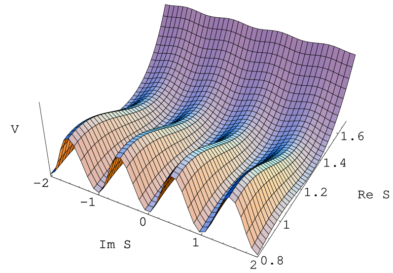
Figure 1: The scalar $S$-dual potential $V(S,S^{+})$, Eq. (5), as a function of $({\bf Re}~{}S,{\bf Im}~{}S)$.

where $S_{R}=2~{}{\bf Re}~{}S$. The function $\eta(S)=q^{1/24}\prod_{n}(1-q^{n})$ is the Dedekind function, $q\equiv\exp(-2\pi S)$; $\hat{G}_{2}(S)=G_{2}(S)-2\pi/S_{R}$ is the weight two Eisenstein function and $G_{2}(S)=\frac{1}{3}\pi^{2}-8\pi^{2}\sum_{n}\sigma_{1}(n)\exp(-2\pi nS)$, where $\sigma_{1}(n)$ is the sum of the divisors of $n$. The potential (5) is shown in Figure 1.

To this potential (5) one has to add the contribution of $D$-terms associated with the gauge sector of the theory. We shall assume that these fields are in their ground state and hence the contribution from $D$-terms will amount to a constant contribution to the potential (5) once the field $S$ itself is settled in its ground state. The contribution from the $D$-terms can be written in an $S$-modular invariant form,

$$V_{D}=\frac{1}{2~{}{\bf Re}~{}f}\,D^{2}\ ,$$ (6)

where $D=\hat{g}K^{i}{T_{i}}^{j}\Phi_{j}+\xi$, $\hat{g}$ being the gauge charge, ${T_{i}}^{j}$ are the generators of the gauge group and $\xi$ is the Fayet-Illiopoulos term. $S$-modular invariance is ensured for $f=\frac{1}{2\pi}[\ln(j(S)-744]$, $j(S)$ being the generator of modular invariant functions and where for large $S$ one has $j(S)=\frac{1}{q}+744+196884q+O(q^{2})$, with $q=e^{-2\pi q}$ [11, 29]. From string perturbative results it follows that $f=S$ and hence, $S$-duality implies that $f\rightarrow f$. Another possible realization for ensuring $S$-duality is $f\rightarrow 1/f$, although this requires the existence of the so-called “magnetic condensate” [21, 29].

Let us now turn to the discussion of the geometrical setting of our model. We shall restrict ourselves to spatially homogeneous and isotropic field configurations. A general discussion of the field configurations associated with the geometry we shall use, based on the theory of symmetric fields, can be found in Refs. [30, 31]. The most general form of the metric is

$$ds^{2}=-N^{2}(t)dt^{2}+a^{2}(t)\sum_{i=1}^{3}\omega^{i}\omega^{i}~{},$$ (7)

where the scale factors $a(t)$ and the lapse function $N(t)$ are arbitrary non-vanishing functions of time, $\omega^{\alpha}$ denote local moving coframes in $S^{3}$ and $\sum_{i=1}^{3}\omega^{i}\omega^{i}$ coincides with the standard metric $d\Omega_{3}^{2}$ of a 3-dimensional sphere.

Consistency with the geometry requires that the field $S$ depends just on time:

$$S(t,x^{i})=S(t).$$ (8)

Substituting the ansätze (7) and (8) into the action (4), we obtain a one-dimensional effective action:

$$S_{\rm eff}[a,S,S^{+}]=2\pi^{2}\int dt~{}\left[6~{}a~{}N(\left(\frac{\dot{a}}{N}\right)^{2}-1)-\frac{N~{}a^{3}}{(S+S^{+})^{2}}~{}\frac{\dot{S}}{N}~{}\frac{\dot{S^{+}}}{N}-N~{}a^{3}~{}\hat{V}(S,S^{+})\right]~{},$$ (9)

where $\hat{V}(S,S^{+})=V(S,S^{+})+V_{D}$ for constant gauge fields $\Phi_{j}$.

The canonical conjugate momenta associated with the canonical variables are the following:

$$\Pi_{a}=24\pi^{2}~{}a~{}\frac{\dot{a}}{N}~{},~{}\Pi_{S}=-2\pi^{2}\frac{a^{3}}{(S+S^{+})^{2}}~{}\frac{\dot{S^{+}}}{N}~{},~{}\Pi_{S^{+}}=-2\pi^{2}\frac{a^{3}}{(S+S^{+})^{2}}~{}\frac{\dot{S}}{N}~{}.~{}$$ (10)

The minisuperspace Hamiltonian density, in the $N=1$ gauge, is given by:

$${\cal H} = \Pi_{a}~{}\dot{a}+\Pi_{S}~{}\dot{S}+\Pi_{S^{+}}~{}\dot{S^{+}}-{\cal L}$$

$$= \frac{1}{48\pi^{2}a}~{}\Pi_{a}^{2}-\frac{(S+S^{+})^{2}}{2\pi^{2}a^{3}}~{}\Pi_{S}~{}\Pi_{S^{+}}+2\pi^{2}a(6+a^{2}~{}\hat{V}(S,S^{+}))~{}.$$

Canonical quantization then follows by promoting the conjugate momenta into operators:

$$\Pi_{a}\mapsto-i\frac{\partial}{\partial\,a}~{},\Pi_{S}\mapsto-i\frac{\partial}{\partial\,S}~{},\Pi_{S^{+}}\mapsto-i\frac{\partial}{\partial\,S^{+}}~{}.$$ (12)

Finally, one obtains the Wheeler-DeWitt equation:

$$\left[\frac{\partial^{2}}{\partial a^{2}}-\frac{24~{}(S+S^{+})^{2}}{a^{2}}\frac{\partial^{2}}{\partial S~{}\partial S^{+}}-96~{}\pi^{4}~{}a^{2}~{}(6+a^{2}~{}\hat{V}(S,S^{+}))\right]\Psi[a,S,S^{+}]=0~{},$$ (13)

where in the usual parameterization of the factor ordering ambiguity, $\pi_{a}^{2}\mapsto-a^{-p}\frac{\partial}{\partial a}\left(a^{p}\frac{\partial}{\partial a}\right)$, we have set $p=0$. Of course, our results will not depend on this choice as a change in the ordering of operators amounts only to a change in the normalization of the wave function.

Given the importance of the $S$-modular invariance in the ${\cal N}=1$ supergravity model we are studying, it would be more than natural to consider the wave function of the Universe in terms of explicitly $S$-invariant modular forms. Actually, the conservation law associated to $S$-modular invariance seems to imply that $S$ and $S^{+}$ should appear in the wave function only through $S$-modular invariant combinations. The $S$-modular invariant forms present in our model via the potential (5), are the following:

$$X(S,S^{+})\equiv(S+S^{+})|\eta(S)|^{4}=S_{R}|\eta(S)|^{4}~{}$$ (14)

and

$$Y(S,S^{+})\equiv(S+S^{+})^{2}|\hat{G}_{2}(S)|^{2}=S_{R}^{2}~{}|\hat{G}_{2}(S)|^{2}~{}.$$ (15)

Hence, one might assume that $\Psi[a,S,S^{+}]=\Psi[a,{\cal X},{\cal Y}]$, where ${\cal X}={\cal X}(X,Y)$ and ${\cal Y}={\cal Y}(X,Y)$ are $S$-modular invariant combinations of $X$ and $Y$. This statement would imply, as shown in [28], that any bare cosmological constant would have to vanish in order to preserve the $S$-modular invariance. We shall see, however, that this is not so if the cosmological constant arises, as in our model, from an explicitly $S$-modular invariant potential and if in this process $S$-modular invariance is spontaneously broken down to some smaller symmetry – as we shall discuss below. Before pursuing this issue, let us show that the dependence of the wave function on $S$-modular invariant structures is more involved than what we have previously suggested. Indeed, starting from the relation between $\eta(S)$ and $G_{2}(S)$ [21],

$$G_{2}(S)=-\frac{4\pi}{\eta(S)}~{}\frac{\partial\eta(S)}{\partial S}~{},$$ (16)

one finds,

$$\frac{\partial^{2}X(S,S^{+})}{\partial S~{}\partial S^{+}}=\frac{1}{4\pi^{2}}~{}X(S,S^{+})~{}|\hat{G}_{2}(S)|^{2}~{},$$ (17)

that involves $G_{2}(S)$. This means that if we initially assume that the wave function of the Universe depends upon $X(S,S^{+})$, then it must also depend on $Y(S,S^{+})$. To realize that such is true, one just has to assume otherwise, and after a simple calculation such as

$$\frac{\partial^{2}\Psi[a,X(S,S^{+})]}{\partial S~{}\partial S^{+}}=\frac{|\hat{G}_{2}(S)|^{2}}{4\pi^{2}}\left[X^{2}~{}\frac{\partial^{2}\Psi[a,X]}{\partial^{2}X}+X~{}\frac{\partial\Psi[a,X]}{\partial X}\right]~{},$$ (18)

one immediately sees that this is not coherent as the Wheeler-DeWitt equation now involves more modular structures than initially assumed. So, our initial assumption of $\Psi[a,S,S^{+}]=\Psi[a,{\cal X},{\cal Y}]$, with ${\cal X}={\cal X}(X,Y)$ and ${\cal Y}={\cal Y}(X,Y)$ seems reasonable. However, from a similar line of thought as the previous one, we shall see that even more modular structures are needed.

Indeed, as one computes the differential operators of the Wheeler-DeWitt equation under the previous assumption for the wave function, one finds that the derivative ${\partial\over\partial S}Y(S,S^{+})$ appears as part of such operators, and such derivative depends upon ${\partial\over\partial S}\hat{G}_{2}(S)$. Now, from the the covariant derivative of a modular form of weight $d$, $F_{d}$, $D_{d}F_{d}=F_{d+2}$, where $D_{d}\equiv\frac{i}{\pi}\frac{\partial}{\partial S}+\frac{d}{2\pi S_{R}}$ it follows that

$$D_{2}\hat{G}_{2}=\frac{1}{6}G_{4}-\frac{1}{6}{\hat{G}_{2}}^{2}~{}~{},~{}~{}~{}~{}~{}D_{4}G_{4}=\frac{2}{3}G_{6}-\frac{2}{3}\hat{G}_{2}G_{4}~{}~{},~{}~{}~{}~{}~{}D_{6}G_{6}=G_{4}^{2}-\hat{G}_{2}G_{6}~{}~{},~{}$$ (19)

and so on. This then implies that the derivatives of the modular structures according to $S$ and $S^{+}$, present in the Wheeler-DeWitt equation, will give origin to terms involving a new modular invariant form involving $G_{4}$, say $Z(S,S^{+})\equiv(S+S^{+})^{4}|\hat{G}_{4}(S)|^{2}$. This should have to be considered in the wave function, implying that ${\cal X}={\cal X}(X,Y,Z)$ and ${\cal Y}={\cal Y}(X,Y,Z)$. Of course, this new modular invariant structure via derivative terms would give origin to a modular structure involving $G_{6}$ which should be included into the wave function and so on. One concludes then that the whole Eisenstein series should be involved and that considering modular invariant structures to obtain the wave function of the Universe is not a very practical procedure.

In the next section we shall study the boundary conditions of the Wheeler-DeWitt equation and look for solutions of equation (13) that depend explicitly on $S$ and $S^{+}$ in the limits of small and large scale-factor.

3 Solutions of the Wheeler-DeWitt Equation

We start this section by establishing the boundary conditions for the Wheeler-DeWitt equation (13). We shall obtain these boundary conditions through the path integral representation for the ground-state of the Universe in a compact manifold $C$ [17],

$$\Psi[a,S,S^{+}]=\int_{C}{{\cal D}[a]{\cal D}[S]{\cal D}[S^{+}]\exp(-S_{\rm E})}~{},$$ (20)

which allows evaluating $\Psi(a,S,S^{+})$ close to $a=0$. Notice that since one can have, via an appropriate choice of the metric, $\Psi[a,S,S^{+}]=e^{-S_{E}}$ near the past null infinity $\cal I^{-}$, the procedure we are using here is really the most suitable one. The Euclidean action, $S_{\rm E}=-iS_{\rm eff}$, is obtained through the effective action (9) taking $d\tau=iNdt$ such that the Euclidean metric is compact

$$\hat{ds^{2}}=d\tau^{2}+a^{2}(\tau)\sum_{i=1}^{3}\omega^{i}\omega^{i}~{}.$$ (21)

In order to estimate $\Psi[a,S,S^{+}]$ close to $a\rightarrow 0$ one evaluates $S_{E}$ from $\tau=0$ to $\Delta\tau$:

$$S_{E}=2~{}\pi^{2}\int_{0}^{\Delta\tau}{d\tau\left[6~{}a~{}(\dot{a}^{2}+1)-\frac{a^{3}}{S_{R}^{2}}~{}\dot{S}~{}\dot{S^{+}}+a^{3}~{}\hat{V}(S,S^{+})\right]}~{}.$$ (22)

Close to $\tau=0$, $a(\tau)\approx\tau$, then

$$S_{E}=2~{}\pi^{2}\int_{0}^{\Delta\tau}{d\tau\left[12~{}\tau-\frac{\tau^{3}}{S_{R}^{2}}~{}\dot{S}~{}\dot{S^{+}}+\tau^{3}~{}\hat{V}(S,S^{+})\right]}~{},$$ (23)

which yields for regular $S$, $S^{+}$ and $\hat{V}(S,S^{+})$ and non-vanishing $S$ that $S_{E}\rightarrow 0$ as $\Delta\tau\rightarrow 0$ and hence that $\Psi[a,S,S^{+}]\rightarrow 1$. For vanishing $S$ and for $S\to\infty$ it follows that $\hat{V}(S,S^{+})\to\infty$ implying that $\Psi[a,S,S^{+}]\rightarrow 0$.

In order to proceed one should also have to establish the regions where the solution of the Wheeler-DeWitt equation is oscillatory or exponential. This can be done studying the regions where, for surfaces of constant minisuperspace potential $U\equiv 96\pi^{4}a^{2}(6+a^{2}~{}\hat{V}(S,S^{+}))$, the minisuperspace metric $ds^{2}=-~{}da^{2}+dS~{}dS^{+}$ is either spacelike $ds^{2}<0$ or timelike $ds^{2}>0$ (see for instance [27] and references therein). However, as we are going to discuss soon, we shall use the scale-factor duality to obtain the very early Universe wave function from the very late Universe wave function and hence this study is not so crucial. Nevertheless, we shall discuss in section 4 how, via the study of the square of the trace of the extrinsic curvature, $K^{2}=K_{ij}K^{ij}$, one can determine whether the wave function corresponds to a Lorentzian or to an Euclidean geometry.

We are now ready to start studying solutions to the Wheeler-DeWitt equation. As an exact solution to the full equation is not possible to obtain, we shall study particular solutions under certain particular regimes of the evolution of the Universe. Namely we shall look at four distinct approximations: what we call the very early Universe, i.e., when we have $a<<1$, and whose solution shall be denoted by $\Psi^{(--)}$; the early Universe, i.e., when we have $a<1$ but not $a<<1$ (such that $a^{2}>>a^{4}$), and whose solution shall be denoted by $\Psi^{(-)}$; the late Universe, i.e., when we have $a>1$, and whose solution shall be denoted by $\Psi^{(+)}$; and the very late Universe, i.e., when we have $a>>1$ and $a^{4}>>a^{2}$, and whose solution shall be denoted by $\Psi^{(++)}$.

From the boundary condition one can search for solutions relevant for the early Universe, namely when $a<1$, but with $a^{2}>>a^{4}$ in order to avoid the $a=0$ curvature singularity. The wave function can be separated as $\Psi(a,S,S^{+})=A(a)~{}F(S,S^{+})$ and a solution for the Wheeler-DeWitt equation is obtained in terms of Bessel functions:

$$\Psi^{(-)}(a,S,S^{+})=a^{1/2}\left\{k_{1}~{}I_{-1/4}[12\pi^{2}a^{2}]+k_{2}~{}I_{1/4}[12\pi^{2}a^{2}]\right\}~{}~{},$$ (24)

where the integration constants $k_{1}$ and $k_{2}$ are given in terms of $~{}F(S,S^{+})$ which was maintained fixed. This implies that under the latter conditions, that is fixed $~{}F(S,S^{+})$, the wave function predicts an expanding Universe.

A solution for the very early Universe can be obtained from a solution for the very late Universe through the scalar-factor duality, with an appropriate shift in the real part of the $S$-field such that it corresponds to a sub-set of modular transformations (1) for this field. We obtain in this case the following wave function:

$$\Psi^{(--)}(a,S,S^{+})=a^{-1/2}\left\{c_{1}~{}I_{-1/6}[\frac{1}{3}(96\pi^{4}\hat{V})^{1/2}a^{-3}]+c_{2}~{}I_{1/6}[\frac{1}{3}(96\pi^{4}\hat{V})^{1/2}a^{-3}]\right\}~{},$$ (25)

where $c_{1}$ and $c_{2}$ are constants. This wave function indicates that the most likely configuration for the fields $S$ and $S^{+}$ is the one where they sit at the top of $\hat{V}$, as the probability of a given configuration is given by $|\Psi|^{2}$. This result is consistent with the assumption of Ref. [13] when computing the scalar and tensor perturbations, that is energy density fluctuations and gravitational waves, generated by the $S$ field during inflation. As discussed in [12], inflation of the topological type can take place in models with $S$-modular invariance due to the presence of domain walls separating different vacua of the theory. This possibility has been discussed in generical terms by Linde [32] and Vilenkin [33] and it was suggested in the context of string cosmology [34] in order to solve the Polonyi problem [35] due to moduli fields. Thus, quantum cosmology does support the assumption considered in the topological inflationary model of [16, 12], built in the context of an $S$-modular invariant ${\cal N}=1$ supergravity, that the field $S$ starts at the top of $\hat{V}$ before inflation takes place. It should be pointed out that, as shown in Refs. [12, 13], a realistic model requires that both $S$ and $T$ dualities are considered in order to match the amplitude of energy density fluctuations as observed by COBE. Moreover, it was shown in [13] that from the latter requirement and from COBE bounds for the spectral index of scalar perturbations, $0.7<n_{s}<1.2$, it follows that the spectrum of tensor perturbations is nearly flat, which is consistent with observations and that its amplitude is fairly modest $A_{t}\sim 10^{-2}A_{s}$. This contrasts, for instance, with what is expected from the Pre-Big-Bang model [7].

Let us now turn to the problem of the cosmological constant. It has been argued by many authors that $S$-duality may play an important role in the vanishing or smallness of the cosmological constant. Indeed, for instance, Witten [36] has recently conjectured that via a duality transformation, a 4-dimensional field theory could be related to a 3-dimensional one with the advantage that in the latter the breaking of supersymmetry, a condition imposed upon by phenomenology, does not imply that the cosmological constant is non-vanishing. In Ref. [28], it was shown that introducing a bare cosmological constant in the action implies that the resulting equations of motion lose the invariance under $S$-duality, unless one has vanishing cosmological constant. Therefore, it follows that, within string theory, the naturalness principle of ’t Hooft [37] can be satisfied as the vanishing of the cosmological constant implies that the theory has more symmetry, namely $S$-duality. Our work shows however that the situation is more complex, as the cosmological constant has to arise from a potential term and this should be, as we have been explicitly considering, modular invariant, that is invariant under $SL(2,\bf{Z})$ transformations. Furthermore, the process of symmetry breaking has also to be taken into account. From Figure 1 one sees that the potential has an infinite number of minima located at the points ${\bf Im}~{}S\in{\bf Z}$ and ${\bf Re}~{}S=0.8$ or ${\bf Re}~{}S=1.3$. Indeed, as the components of the $S$ field settle in the ground state, $SL(2,\bf{Z})$ is broken down to ${\bf Z}_{\infty}$. After this spontaneous symmetry breaking of modular invariance, we still have axion fluctuations about the degenerate minima. Recall that $\chi={\bf Im}~{}S$ is the axion field, and one can represent axion oscillations about the several minima as governed by the following potential, near all $n$ and near both $\langle{\bf Re}~{}S\rangle$, written as (see Figure 1):

$$V(S,S^{+})=\alpha(\langle{\bf Re}~{}S\rangle)~{}[{\bf Im}~{}S-n]^{2}~{},~{}~{}~{}~{}n\in{\bf Z}~{},$$ (26)

where $\alpha(\langle{\bf Re}~{}S\rangle)=\{\alpha(0.8),\alpha(1.3)\}=\{\alpha_{-},\alpha_{+}\}\equiv\alpha(j)$. So, the potential depends on the integer $n$ and the choice of factor $\alpha(j)$. We can therefore label each vacua as $|jn\rangle$, where the potential is $V_{jn}=\alpha(j)[\chi-n]^{2}$.

Moreover, this implies that we have a $\theta$-vacua which can be labeled by the quantum numbers $|jn\rangle$. Thus, the ground-state wave function is a quantum superposition over all the absolute minima of the modular invariant scalar potential:

$$\Psi(a,S,S^{+})=\sum_{j=\pm}\sum_{n\in{\bf Z}}c_{jn}\Psi_{jn}(a,S,S^{+})~{}.$$ (27)

The wave function for each state $|jn\rangle$ can be computed with the help of the WKB approximation (and in the late Universe approximation), that is

$$\Psi^{(+)}(a,S,S^{+})=N\exp\{iS(a,S,S^{+})/{\hbar}\}.$$ (28)

At one-loop level the wave function can be easily obtained:

$$\Psi_{jn}^{(+)}(a,S,S^{+})=\frac{N(S,S^{+})}{a^{1/2}~{}[\langle\hat{V}_{jn}\rangle a^{2}+6]^{1/4}}\exp\left\{-{4~{}\sqrt{6}~{}\pi^{2}\over 3~{}{\hbar}~{}\langle\hat{V}_{jn}\rangle}~{}[\langle\hat{V}_{jn}\rangle a^{2}+6]^{3/2}+{\cal O}({\hbar})\right\}~{},$$ (29)

where $N(S,S^{+})$ is a normalization constant that depends on values of $S$ and $S^{+}$ at the minimum.

The most striking feature of this wave function is that it is sharply peaked at $\langle\hat{V}\rangle\rightarrow 0^{-}$, implying that the most likely field configurations for expanding Universes are the ones consistent with this condition. Of course, this is reminiscent of the earlier ideas of Baum, Hawking and Coleman [38, 39, 40]. In [40] it was shown that the inclusion of wormhole type solutions in the Euclidean path integral allows for treating the contribution of inequivalent topological configurations to the wave function of the Universe. After using the dilute gas approximation to compute the instanton-wormhole contribution to the Euclidean effective action it was shown that the parameters of the effective theory, such as the cosmological constant, the gravitational constant, etc., turn into dynamical variables whose values are fixed once the wave function is maximized. It was also argued by Coleman that the inclusion of the wormhole contribution to the Euclidean path integral would fix the normalization problem that rendered the proposal of Baum and Hawking inconsistent. This point however, has been criticized on various grounds, specially in what concerns the fact that Euclidean quantum gravity is, for a vanishing cosmological constant, unbounded from below from which it follows that the theory does not have a stable ground state (see e.g. Ref. [41] for a thorough discussion). Despite all these issues, we stress that our analysis indicates that $S$-modular invariance at the quantum level implies that the cosmological constant problem in ${\cal N}=1$ supergravity strongly resembles the strong CP problem. In the latter, the $\theta$ angle is adjusted to vanish thanks to the Peccei-Quinn field associated to an extra $U(1)_{PQ}$ symmetry. Adjusting mechanisms for the vanishing of the cosmological constant inspired on the Peccei-Quinn mechanism have been envisaged [42], although strong arguments on the lack of effectiveness of such mechanisms have been put forward [43].

Thus, we have seen in this section that our analysis of the solutions of Wheeler-DeWitt equation for a modular invariant ${\cal N}=1$ supergravity model in an homogeneous and isotropic spacetime does shed some light into the issue of the initial conditions for the onset of energy density fluctuations generated at the topological inflationary scenario discussed in Ref. [13] and also into the problem of the cosmological constant and its striking resemblance with the strong CP problem.

4 Interpretation of the Wave Function

The behavior of the wave function we have obtained in the previous section can be analyzed using the square of the trace of the extrinsic curvature, $K^{2}=K_{ij}K^{ij}$, which allows establishing whether the wave function in the semiclassical limit corresponds to a Lorentzian or to an Euclidean geometry. Of course, the Wheeler-DeWitt equation is the same whether Lorentzian or Euclidean metrics are used to derive it. The extrinsic curvature is a measure of the variation of the normal to the hypersurfaces of constant time, and is given in general by:

$$K_{ij}=N^{-1}\left(-\frac{1}{2}\frac{\partial h_{ij}}{\partial t}+\nabla_{j}N_{i}\right)~{},$$ (30)

where $h_{ij}$ is the $3$-metric and $N_{i}$ are the components of the shift-vector. For our geometry (7) we have

$$K_{ij}=-\frac{\dot{a}}{a}h_{ij}~{},$$ (31)

and

$$K^{2}=-\frac{1}{192\pi^{4}a^{4}}{\partial^{2}\over\partial a^{2}}~{}.$$ (32)

Hence, in order to interpret the wave function we have to consider the following quantity:

$$W\Psi(a,S,S^{+})\equiv\frac{K^{2}\Psi(a,S,S^{+})}{\Psi(a,S,S^{+})}~{}.$$ (33)

If $W$ is positive it implies the wave function is oscillatory and therefore it corresponds to a classical and Lorentzian geometry. If, on the other hand, $W$ is negative, then the wave function is “exponential” or of tunneling type corresponding to a quantum or Euclidean geometry. A rather straightforward computation indicates that $W\Psi(a,S,S^{+})$ behaves as follows:

Very Early Universe:

$$W\Psi^{(--)}(a,S,S^{+})<0~{};$$ (34)

Early Universe:

$$W\Psi^{(-)}(a,S,S^{+})<0~{};$$ (35)

Late Universe:

$$W\Psi^{(+)}(a,S,S^{+})>0~{}.$$ (36)

These results indicate that the transition from the quantum to classical regime occurs for $a>1$ after which the quartic term in the scale factor in the minisuperspace potential, $U(a,S,S^{+})\equiv-96\pi^{4}a^{2}(6+a^{2}~{}\hat{V}(S,S^{+}))$, dominates the quadratic one arising from the spatial curvature. Moreover, in the oscillatory or classical region the wave function can be further analyzed using the WKB approximation, $\Psi=Ce^{iI}$, where $C$ is a slowly varying factor and $I$ a rapidly varying phase. The phase $I$ is chosen so that it satisfies the Hamilton-Jacobi equation:

$$-\left(\frac{\partial I}{\partial a}\right)^{2}+\frac{24~{}(S+S^{+})^{2}}{a^{2}}\left(\frac{\partial I}{\partial S~{}}\right)\left(\frac{\partial I}{\partial S^{+}}\right)+U(a,S,S^{+})=0~{}.$$ (37)

The meaning of the phase $I$ can be understood acting with the operators $\Pi_{a}$, $\Pi_{S}$ and $\Pi_{S^{+}}$ on the wave function. Indeed, for instance, operating with $\Pi_{a}$ (the procedure is analogous for $\Pi_{S}$ and $\Pi_{S^{+}}$) yields:

$$\Pi_{a}\Psi=\left[\frac{\partial I}{\partial a}-i\frac{\partial\ln C}{\partial a}\right]\Psi~{},$$ (38)

and one realizes that, since in the WKB approximation

$$\left|\frac{\partial I}{\partial a}\right|\gg\left|\frac{\partial}{\partial a}\ln C\right|~{}~{},$$ (39)

then

$$\Pi_{a}=\frac{\partial I}{\partial a}~{}~{},~{}~{}\Pi_{S}=\frac{\partial I}{\partial S}~{}~{},~{}~{}\Pi_{S^{+}}=\frac{\partial I}{\partial S^{+}}~{}~{}.$$ (40)

Hence the wave function corresponds in this situation to a three-parameter subset of solutions of (37) and can be interpreted as a boundary condition for the classical solutions.

5 Discussion and Conclusions

In this paper we have obtained solutions of the Wheeler-DeWitt equation from the minisuperspace model resulting from imposing $S$-modular invariance in the bosonic sector of ${\cal N}=1$ supergravity, assuming a closed Friedmann-Robertson-Walker spacetime. In section 2 we have introduced the specificities of the model that were associated with the modular invariance, obtained the Wheeler-DeWitt equation of our problem and outlined our strategy in searching for its solutions. We have implemented the no-boundary Hartle-Hawking proposal in section 3 and addressed the issues of initial field configurations at the very early Universe and of the cosmological constant. The former discussion is, of course, relevant when studying the onset of inflation and the very early Universe conditions that have given rise to the energy density fluctuations and gravitational waves generated by inflation. We have used the scalar-factor duality to obtain the wave function for this case and have shown that, for an expanding Universe, the most likely configuration for the $S$ field was the one where it started sitting at the top of the modular invariant ${\cal N}=1$ supergravity potential. This is consistent with assumptions assumed in Ref. [13] in the context of a topological inflationary model built in an $S$ and $T$ dual ${\cal N}=1$ supergravity model. In order to address the cosmological constant problem we have calculated the wave function of the Universe in the limit of very large scale-factor and we have shown that the wave function is sharply peaked, after spontaneous symmetry breaking of the $SL(2,\bf{Z})$ modular invariance down to ${\bf Z}_{\infty}$, at a vanishing potential from below. This feature is common to known solutions for the cosmological constant problem [38, 39, 40], but with the novelty that, given the ground-state structure of dual ${\cal N}=1$ supergravity, there is actually a $\theta$-vacuum which suggests that the cosmological constant problem has, at the quantum level, a great resemblance with the strong CP problem.

Finally, we have identified, in section 4, the regimes where the wave function is Lorentzian or Euclidean applying the operator $K^{2}=K_{ij}K^{ij}$, where $K_{ij}$ is the extrinsic curvature of spacetime manifold, on the wave function. We have further interpreted the classical Lorentzian regime using the WKB approximation and writing the Hamilton-Jacobi equation that the relevant phase must satisfy. We have found that the Universe evolved from a quantum to a classical regime after the scale factor quartic term in the minisuperspace potential dominated the quadratic term. We have also shown that our analysis succeeded in both establishing a quantum mechanical validation of the classical treatment of Refs. [12, 13] concerning topological inflation, as well as hinting some directions in a possible mechanism for explaining the vanishing of the cosmological constant in the late Universe.

Acknowledgments

One of us (R.S.) is supported in part by funds provided by the U.S. Department of Energy (D.O.E.) under cooperative research agreement $\sharp$DE-FC02-94ER40818, in part by Fundação Calouste Gulbenkian (Portugal), and in part by the Fundação Luso-Americana para o Desenvolvimento grant 50/98 (Portugal).

References

- [1] J.H. Schwarz, in “Elementary Particles and the Universe, Essays in honor of M. Gell-Mann”, J. Schwarz ed. (Cambridge, 1991).
- [2] K.S. Narain, Phys. Lett. B169 (1986) 41; K.S. Narain, M.H. Sarmadi and E. Witten, Nucl. Phys. B279 (1987) 369.
- [3] E. Alvarez and M. Osorio, Phys. Rev. D40 (1989) 1150.
- [4] G. Veneziano, Phys. Lett. B265 (1991) 287; A.A. Tseytlin, Mod. Phys. Lett. A6 (1991) 1721.
- [5] X.C. de la Ossa and F. Quevedo, Nucl. Phys. B403 (1993) 377.
- [6] M. Gasperini and G. Veneziano, Astropart. Phys. 1 (1993) 317.
- [7] G. Veneziano, Phys. Lett. B406 (1997) 297.
- [8] J. Hwang, Astropart. Phys. 8 (1998) 201; M.S. Turner and E.J. Weinberg, Phys. Rev. 56 (1997) 4604; D. Coule, Class. Quantum Gravity 15 (1998) 2803; N. Kaloper, A. Linde and R. Bousso, “Pre-Big-Bang Requires the Universe to be Exponentially Large from the Very Beginning”, hep-th/9801073; J. Soda, M. Sakagami and S. Kawai, “Novel Instability in Superstring Cosmology”, gr-qc/9807056.
- [9] N. Kaloper, R. Madden and K.A. Olive, Nucl. Phys. , B452 (1995) 677; Phys. Lett. B371 (1996) 34.
- [10] T. Damour and A. Vilenkin, Phys. Rev. D53 (1996) 2989; G.G. Ross and S. Sarkar, Nucl. Phys. B461 (1996) 597; M.C. Bento and O. Bertolami, Phys. Lett. B365 (1996) 59.
- [11] A. De La Macorra and S. Lola, Phys. Lett. B373 (1996) 299.
- [12] M.C. Bento and O. Bertolami, Phys. Lett. B384 (1996) 98.
- [13] M.C. Bento, O. Bertolami and N.J. Nunes, Phys. Lett. B427 (1998) 261.
- [14] A.A. Tseytlin and C. Vafa, Nucl. Phys. B372 (1992) 443.
- [15] O. Bertolami, Nucl. Phys. B57 (Proc. Suppl.) (1997) 91.
- [16] M.C. Bento and O. Bertolami, Class. Quantum Gravity 12 (1995) 1919.
- [17] J.B. Hartle and S.W. Hawking, Phys. Rev. D28 (1983) 2960.
- [18] A. Kehagias and A. Lukas, Nucl. Phys. B477 (1996) 549.
- [19] M. Gasperini, J. Maharana and G. Veneziano, Nucl. Phys. B472 (1996) 497; A. Lukas and R. Poppe, Mod. Phys. Lett. A12 (1997) 597; M. P. Da̧browski and C. Kiefer, Phys. Lett. B397 (1997) 185.
- [20] T. Banks, W. Fischler and L. Motl, “Dualities versus Singularites”, hep-th/9811194.
- [21] A. Font, L.E. Ibáñez, D. Lüst and F. Quevedo, Phys. Lett. B245 (1990) 401; B249 (1990) 35.
- [22] A. Sen, Phys. Lett. B329 (1994) 217.
- [23] S.W. Hawking, Nucl. Phys. B239 (1984) 257.
- [24] O. Bertolami and J.M. Mourão, Class. Quantum Gravity 8 (1991) 1271.
- [25] O. Bertolami and P.V. Moniz, Nucl. Phys. B439 (1995) 259.
- [26] P.V. Moniz, Int. J. Mod. Phys. A11 (1996) 4321.
- [27] O. Bertolami, P.D. Fonseca and P.V. Moniz, Phys. Rev. D56 (1997) 4530.
- [28] S. Kar, J. Maharana and H. Singh, Phys. Lett. B374 (1996) 43.
- [29] Z. Lalak, A. Niemeyer and H. P. Nilles, Nucl. Phys. B453 (1995) 100.
- [30] O. Bertolami, J.M. Mourão, R.F. Picken and I.P. Volobujev, Int. J. Mod. Phys. A6 (1991) 4149.
- [31] M.C. Bento, O. Bertolami, P.V. Moniz, J.M. Mourão and P.M. Sá, Class. Quantum Gravity 10 (1993) 285.
- [32] A. Linde, Phys. Lett. B372 (1994) 208.
- [33] A. Vilenkin, Phys. Rev. Lett. 72 (1994) 3137.
- [34] T. Banks, M. Berkooz, S.H. Shenker, G. Moore and P.J. Steinhardt, Phys. Rev. D52 (1995) 3548.
- [35] G.D. Coughlan, W. Fischler, E.W. Kolb, S. Raby and G.G. Ross, Phys. Lett. B131 (1983) 59; J. Ellis, D.V. Nanopoulos and M. Quirós, Phys. Lett. B174 (1986) 176; O. Bertolami and G.G. Ross, Phys. Lett. B183 (1987) 163; O. Bertolami, Phys. Lett. B209 (1988) 277; B. de Carlos, J.A. Casas, F. Quevedo and E. Roulet, Phys. Lett. B318 (1993) 447; M.C. Bento and O. Bertolami, Phys. Lett. B336 (1994) 6; T. Banks, D.B. Kaplan and A.E. Nelson, Phys. Rev. D49 (1994) 779.
- [36] E. Witten, Int. J. Mod. Phys. A10 (1995) 1247.
- [37] G. ’t Hooft, “Under the Spell of the Gauge Principle” (World Scientific 1994) .
- [38] E. Baum, Phys. Lett. B133 (1984) 185.
- [39] S.W. Hawking, Phys. Lett. B134 (1984) 403.
- [40] S. Coleman, Nucl. Phys. B307 (1988) 867.
- [41] W. Fischler, I. Klebanov, J. Polchinski and L. Susskind, Nucl. Phys. B237 (1989) 157.
- [42] F. Wilczek, “How far are we from the Gauge Forces”, Proceedings of the 1983 Erice Conference, Ed. A. Zichichi (Plenum Press, New York 1983).
- [43] S. Weinberg, Rev. Mod. Phys. 61 (1981) 1.