On Uniformly Accelerated Black Holes

Abstract

The static and stationary C-metric are revisited in a generic framework and their interpretations studied in some detail. Specially those with two event horizons, one for the black hole and another for the acceleration. We found that: i) The spacetime of an accelerated static black hole is plagued by either conical singularities or lack of smoothness and compactness of the black hole horizon; ii) By using standard black hole thermodynamics we show that accelerated black holes have higher Hawking temperature than Unruh temperature of the accelerated frame; iii) The usual upper bound on the product of the mass and acceleration parameters ($<1/\sqrt{27}$) is just a coordinate artifact. The main results are extended to accelerated rotating black holes with no significant changes.

1 Introduction

Let us mention some relevant aspects of our present knowledge of black holes: The uniqueness theorems[1] lead us to the study of just two families of exact solutions of Einstein equations for stationary vacuum spacetimes– the Schwarzschild’s and Kerr’s, and their charged versions. Distortions and perturbations have been studied during the last two decades[2][3]. In the framework of linearized approximations we learned that the holes response to external perturbations appears as special modes of gravitational waves – the quasi normal ringing modes. Numerical simulations confirm that perturbed black holes settle down by the emission of these modes[5]. There is strong evidence for astrophysical black holes[4] which are perturbed by their environment.

There are also several open issues that have been presented as conjectures: The cosmic censorship conjecture[6], the hoop conjecture [7], the no-hair conjecture [8], the topological censorship conjecture [9] and the adiabatic invariant conjecture [10]. Others have been studied in connection with thermodynamics, statistical mechanics, quantum theory and cosmology [11]. Also examples of more general black holes has been studied in the context of supergravity, string theory and related theories [12].

In this article we study some aspects of accelerated black holes. An interesting feature of these holes is that from a semi-classical view point both Hawking and Unruh radiation may be present because of the horizons associated to the holes and to the acceleration.

The object of our study is an old exact solution of vacuum Einstein equations found in 1917 by Levi-Cività [14] and Weyl [15]. It is a simple and rich geometry. In the seventies, it was found a broader class of exact solution with acceleration and rotation parameters [16] [17] and it was named as C-metric or Weyl C-metric. The solutions were obtained by studying the algebraic properties of special class of geometries. In the eighties, it was known to belong to a general class of boost-rotation symmetric spacetimes[18][19]. These solutions have also charged versions [16] [23]. The charged C-metric is interpreted as the solution for Einstein-Maxwell equations for a charged particle moving with uniform acceleration [16]. Another possible interpretation is the spacetime of two Schwarzschild-type particles joined by a spring moving with uniform acceleration [20].

Actually, the C-metric can be associated to several spacetimes [21]. We review them, in section 2, using a slightly different approach. The most interesting ones have two event horizons and a point singularity. One event horizon has finite area, associated to a black hole and the other event horizon has infinite area, associated to the Rindler horizon of accelerated frames [22]. We compute the surface gravity on these horizons and conclude that, in general, the gravity at the hole is larger than the frame acceleration. We show also, for generic configurations, that the hole’s horizons are not smooth compact surfaces and confirm the well known fact that the line of acceleration is not elementary flat. We remark that the product of surface gravity by the area of the horizon gives exactly the expected mass of the hole. This result is expected because of the coordinate transformation that map the C-metric into a Weyl solution which is a superposition of a hole, with a given mass, and a semi-infinite rod of linear density $1/2$ [24]. Our units are such that $c=G=1$. Finally we notice that the C-metric solution brings no limitation on the acceleration of a black hole. The usual presentation of the solution has the constraint $mA<1/\sqrt{27}$ where $m$ and $A$ are the mass and the acceleration parameters. We show that this constraint is due sole to the choice of coordinates.

In section 3 the rotating C-metric is studied in a similar way. The main new features introduced by a rotation parameter is that it opens the possibility of existence of ergoregions, spinning strings and spinning struts. We extend most of the results of the previous section to include a rotation. The interpretation of the more significant parts of the rotating C-metric is that of a spacetime in the neighborhood of an accelerated Kerr-like particle [25]. We show also that the internal singularity resembles a rotating ring as in the standard Kerr solution.

The amount of gravitational radiation by accelerated black hole is not computed in these paper [26]. As stationary solutions both C and the rotating C metric represent eternal black holes being eternally accelerated with gravitational wave coming from the singularities at infinity in a such amount to balance the output of the accelerated black holes.

In the last section we summarize our main results and make some final comments.

2 The C-metric

Let us first review, in a more general framework, the physical meaning of the vacuum C-metric [14] [27] [21] whose line element is

$$ds^{2}=\frac{1}{A^{2}\left(x+y\right)^{2}}\left[K^{2}F(y)dt^{2}-\frac{dy^{2}}{F(y)}-\frac{dx^{2}}{G(x)}-\frac{G(x)}{K^{2}}d\phi^{2}\right].$$ (1)

All the coordinates and the constant $K$ are dimensionless. The constant $A$ has dimension of inverse of length, which is used to fix the scale of physical interest. The functions $G(x)$ and $F(y)$ are cubic functions such that $G(x)=-F(-x)$. Let us consider the real cubic $Q$ of a real variable $w$

$$Q(w)=\alpha\left(w-w_{1}\right)\left(w-w_{2}\right)\left(w-w_{3}\right).$$ (2)

Let us assume $\alpha>0$ and $Q(w)$ has three real roots $w_{1}<w_{2}<w_{3}$. Setting $G(x)=Q(-x)$ and $F(y)=-Q(y)$, the infinity $x-y$ plane is divided into 16 rectangular regions. Let us suppose the $x$’s range is such that $G(x)\geq 0$. Then, for $-\infty<y<+\infty$ the metric function $F(y)$ changes sign on the roots $w_{1}$, $w_{2}$ and $w_{3}$ and the type of the coordinates $t$ and $y$ are interchanged between time-like and space-like. Now, let us suppose the $y$’s range is such that $F(y)\geq 0$. Then, as $-\infty<x<+\infty$ the other metric function $G(x)$ changes sign on the roots $-w_{3}<-w_{2}<-w_{1}$ and the signature of the metric (1) changes between $-2$ and $+2$. The 2-dimensional spaces $t=const$, $y=w_{k}$, $k=1..3$ can have finite or infinite area which we compute below, while the 2-dimensional spaces $t=const$, $x=-w_{k}$, $k=1..3$ has a vanishing area, that is, it is degenerate into a line (or a point). We can estimate whether or not the length of these lines are finite without knowing the roots explicitly.

$y\;\backslash x$	$x<-w_{3}$	-$w_{3}$	(-$w_{3},$-$w_{2}$)	-$w_{2}$	(-$w_{2},$-$w_{1}$)	-$w_{1}$	-$w_{1}<x$
$y>w_{3}$	-+–(1)	$\infty$	-+++	$\mathcal{L}$	-+–(5)	$\mathcal{L}$	-+++
$w_{3}$	$\infty$		$\infty$		$\mathcal{A}$		$\mathcal{A}$
$(w_{2},w_{3})$	+—(2)	$\infty$	+-++	$\infty$	+—(6)	$\mathcal{L}$	+-++
$w_{2}$	$\mathcal{A}$		$\infty$		$\infty$		$\mathcal{A}$
$(w_{1},w_{2})$	-+–(3)	$\mathcal{L}$	-+++	$\infty$	-+–(7)	$\infty$	-+++
$w_{1}$	$\mathcal{A}$		$\mathcal{A}$		$\infty$		$\infty$
$w_{1}>y$	+—(4)	$\mathcal{L}$	+-++	$\mathcal{L}$	+—(8)	$\infty$	+-++

Table 1: In the first column and in the first row the $y$ and $x$ range are displayed. The second, fourth, sixth and eight columns have the signature of the C-metric depending on the sign of the functions $F(y)$ and $G(x)$. On the roots $y=w_{k}$ the area of the event horizons are shown as finite $\mathcal{A}$ or $\infty$. On the roots $x=-w_{k}$ the lenght of the lines are shown as finite $\mathcal{L}$ or $\infty$. The table is symmetric about $x+y=0$. For comparison see similar tables in [22]

In Table I we present the signature associated to the metric (1) depending on the range of the coordinates $(t,y,x,\phi)$. The event horizons associated to the Killing vector $\xi=A\partial_{t}$ are the roots of $F(y)$. The regions on the same column are divided by Killing horizons at the roots $y=w_{j},\;j=1,2,3$ . The regions on the same rows are disconnected because they have different global signature. They are separated by the roots $x=-w_{k},\;k=1,2,3$. We assume the range of the other coordinates as $0\leq\phi\leq 2\pi$ and $-\infty<t<\infty$ . Thus, the physically meaningful spacetimes are those in which $\phi$ is a space-like coordinate. Thus the $x$ range has to be either $-\infty<x<-w_{3}$ or $-w_{2}<x<-w_{1}$ and the associated spacetimes have signature $-2$. Therefore the regions where Killing vector $\xi=A\partial_{t}$ is time-like represent static and axially symmetric spacetimes and they must belong to the Weyl class[28]. One can divide the $x-y$ plane in a similar way for the case $\alpha$ $<0$.

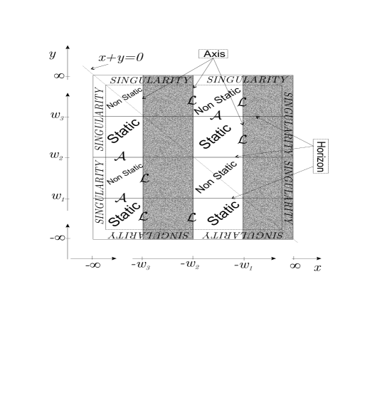
Figure 1: The $x-y$ plane for the C-metric. The vertical separator lines are axis and the horizontal ones are horizons. For comparison see similar figure in [22].

See also Figure 1.

The physical contents can be shown by the scalar invariants [29]. The simplest non-vanishing ones for the C-metric are [30]

$$C_{abcd}C^{abcd} =12\alpha^{2}A^{4}\left(x+y\right)^{6}$$ (3)

$$C_{abcd}C^{cdef}C_{ef}^{\;\;ab} =12\alpha^{3}A^{6}\left(x+y\right)^{9}$$ (4)

where $C_{abcd}$ is the Weyl conformal tensor. Therefore, locally, the only physically meaningful constants are $\alpha$ and $A$. They are called dynamical parameters [17] in contrast to the kinematical ones: $w_{1},w_{2},w_{3}$ and $K$. Furthermore, the spacetimes are not singular at the horizons. They have only singularities at $\left(x+y\right)\rightarrow\pm\infty$. We use below the notation $w_{0}=-\infty$ and $w_{4}=+\infty$.

We can introduce, for future convenience, another constant $m$ with dimension of length such that

$$\alpha=2mA.$$

Therefore the spacetimes have two dimensional dynamical parameters $m$ and $A$. They are associated to mass and acceleration parameters respectively. The two independent limiting cases $m\rightarrow 0$ and $A\rightarrow 0$ have been reported in the literature. The former is an accelerated frame while the latter is a black hole. The cubic degenerates into a quadratic or a linear function. A new justification of this interpretation is given below.

Let us compute the area of the horizons at $y=w_{j}$ where $F(y)=0$ by integrating $x$ and $\phi$ in the their ranges

$$\mathcal{A}_{(j)}^{[k+1,k]}=\frac{2\pi}{A^{2}K}\int_{-w_{k+1}}^{-w_{k}}\frac{dx}{\left(x+w_{j}\right)^{2}}=\frac{2\pi}{A^{2}K}\frac{w_{k+1}-w_{k}}{\left(w_{j}-w_{k}\right)\left(w_{j}-w_{k+1}\right)}$$ (5)

Some of the horizons have finite area ($j\neq k$ and $j\neq k+1$) so they are black hole event horizons, while the infinity area ones are acceleration event horizons. The area of the surfaces $y\rightarrow\pm\infty$ vanishes. The symbolic values of the areas are indicated in the Table I and Figure 1.

One can also compute the distance between the horizons along the axis $x=-w_{k}$ such that $dx=dt=0$ and $G(-w_{k})=0$.

$$\mathcal{L}_{(k)}^{[j+1,j]}=\frac{1}{A}\int_{w_{j}}^{w_{j+1}}\frac{dy}{\left|y-w_{k}\right|\sqrt{\left|F(y)\right|}}$$ (6)

The possible values of the distances are presented in the Table I. They may vanish, be infinite or have a finite value, say $\mathcal{L}$, according to the convergence behavior of the integral in (6).

The qualitative interpretation of the regions labeled by $1$ to $8$ in the Table I is as follows. The regions $1-5$ and $8$ are spacetimes with essential singularities. The odd labeled regions are not static. Note the region $3$: It is a compact spacetime with two black holes separated by a finite distance on one side and both boles attached to a singularity on the other side. Note the regions 5 and 6: They represent the interior of a distorted black hole and the exterior of an accelerated black hole respectively. The finite piece of the axis is behind the black hole. In the literature there are some explicit coordinate transformations from some patches of the C-metric to accelerated black holes, double black holes at infinity, infinity black hole plus black holes and so on [20] [22].

Let us suppose $Q(w)$ has only one real root $w^{\ast}$. As above, set $G(x)=Q(-x)$ and $F(y)=-Q(y)$. Then the $x-y$ plane is divided into 4 rectangular regions.

	$x<-w^{\ast}$	$x=-w^{\ast}$	$x>-w^{\ast}$
$y>w^{\ast}$	$-+--$	$\infty$	$-+++$
$y=w^{\ast}$	$\infty$		$\infty$
$y<w^{\ast}$	$+---$	$\infty$	$+-++$

Table 2: In the first column and in the first row the $y$ and $x$ range are displayed. Single root case. The second and fourth columns have the signature of the C-metric for the coordinates $(t,y,x,\phi)$ depending on the sign of the metric functions $F(y)$ and $G(x)$. On the root $y=w^{*}$ the area of the event horizons are $\infty$. On the root $x=-w^{*}$ the lenght of the lines are $\infty$.

There is an infinite area horizon at $y=w^{\ast}$. The distances along $x=-w^{\ast}$ are infinite. Assuming the same character for the coordinates $t$ and $\phi$ as above, we restrict the meaningful spacetime to $x<-w^{\ast}$. The interpretation is that of an accelerated frame with conical singularities along the line of acceleration and essential singularities at infinity. See Table II.

There are of course other intermediate cases for the roots of $Q(w)$, but we resume our discussion about the three real roots case.

We can compute the surface gravity $\kappa$ on the Killing horizons where the Killing vector $\xi=A\partial_{t}$ vanishes, i.e.

$$\kappa^{2} \equiv\left.-\frac{1}{2}\nabla_{\mu}\xi_{\beta}\nabla^{\mu}\xi^{\beta}\right|_{\left|\xi\right|=0}$$ (7)

$$\kappa_{(i)} =\frac{KA}{2}\left|\frac{dF}{dy}\right|_{y=w_{i}}\;$$ (8)

Thus the dynamical parameter $A$ is proportional to the acceleration surface gravity. Note that $\kappa_{1}>\kappa_{2}$ and $\kappa_{3}>\kappa_{2}$, that is, the horizons at $y=w_{1}$ and $y=w_{3}$, which are “closer to the singularities” at $y\rightarrow\pm\infty$, have stronger surface gravity than the “inner” horizon at $y=w_{2}$. In particular for the region 6, the surface gravity $\kappa_{(3)}$ at the black hole is larger than the acceleration $\kappa_{(2)}$. Thus, using the semi-classical analogy between $\kappa_{(3)}$ and the Hawking temperature of a black hole and between $\kappa_{(2)}$ and the Unruh temperature of the accelerating frame one concludes that the black hole is not in thermodynamical equilibrium with the Unruh environment because of its higher temperature.

For generic black holes, the product of the surface gravity by the area of the horizon is proportional to the mass of the hole[2]. From (7) and (5) we get

$$\kappa_{(i)}\mathcal{A}_{(i)}^{[k+1,k]}=4\pi\frac{m\left(w_{k+1}-w_{k}\right)}{2}=4\pi\;Mass$$ (9)

Thus the parameter $m$ is proportional to the mass of the hole.

The Killing axisymmetric vector $\eta=\partial_{\phi}$ has zero norm on the axis of the symmetry.

$$\eta^{2}=\frac{G(x)}{\left[KA\left(x+y\right)\right]^{2}}$$ (10)

Therefore, the roots of the cubic $G(x)$ are indeed the symmetry axis.

Based sole on the identification of the roots and $G(x)$ as the axis one can compute the ratio between the length of a circle by $2\pi$ times its radius of the metric (1). If this ratio is not unity, there is an angle depletion, that is, a conical singularity.

$$\lim_{\varepsilon\rightarrow 0}\frac{\int_{0}^{2\pi}\frac{1}{A\left|-w_{i}+\varepsilon+y\right|}\frac{\sqrt{\left|G(-w_{i}+\varepsilon)\right|}}{K}d\phi}{2\pi\int_{-w_{i}}^{-w_{i}+\varepsilon}\frac{1}{A\left|x+y\right|}\frac{dx}{\sqrt{\left|G(x)\right|}}}=\frac{G_{x}\left(-w_{i}\right)}{2K}$$ (11)

One can choose the constant $K$ in such a way to avoid the conical singularity in a particular piece of the axis. But in general the conical singularity will show up somewhere on the axis. This is a known feature of the boost-rotation symmetric spacetimes in which the C-metric is just one example[19].

It is also instructive to compute the Gaussian curvature $GC$ of the constant $t$ and constant $y$ surface. It is given by

$$GC=A^{2}(2mA(x+y)^{3}+F(y))$$

from which we can use the Gauss-Bonet theorem [31] to obtain the Euler characteristic $\chi$ of the horizon for $-w_{j}<x<-w_{j-1}$ at $y=w_{i}$ where $F(y)=0$.

$$\chi_{{}_{i}}^{[j,j-1]}+b.t. =\frac{1}{2\pi}\int\int GC\frac{dxd\phi}{KA^{2}\left(x+w_{i}\right)^{2}}$$ (12)

$$=\frac{mA}{K}\left(w_{j}-w_{j-1}\right)\left[2w_{i}-\left(w_{j}+w_{j-1}\right)\right]$$

The boundary terms $b.t.$ vanish if the surface is a compact closed smooth surface (CCSS) and the right-hand side of the equation above is an integer number. It is clear that, in general, the horizons are not CCSS, unless we adjust $K$ for this purpose. Of course we can only apply equation (12) if the surface is finite. Simple torus ($\chi=0$) black holes are selected by choosing the roots such that $w_{j}=w_{j-1}$ or $2w_{i}=w_{j}+w_{j+1}$, for example.

Thus the kinematical parameter $K$ can be chosen to either get rid of the conical singularity in a piece the axis or to make the horizon a CCSS, but not both. Using the membrane paradigm for the black holes and the vision of conical singularities as struts or strings we conclude that in order to accelerate a black hole one needs to push it with a strut and pull it with a string carefully enough in order to not make a hole on its horizon. If one just pushes or pulls it, the membrane will be somehow teared and the horizon will not be a CCSS.

Let us focus on the region 6 of Table I: $w_{2}<y<w_{3}$ and $-w_{2}<x<-w_{1}$. It is an accelerated frame with black hole. The Newtonian mass of the finite line source with mass density $\frac{1}{2}$ is $m\left(w_{2}-w_{1}\right)/2$ which is exactly the mass of the hole (9) as calculated above. The ratio between the surface gravity at $y=w_{3}$ to the acceleration at $y=w_{2}$ is $\kappa_{(3)}/\kappa_{(2)}=\left(w_{3}-w_{1}\right)/\left(w_{2}-w_{1}\right)>1$, so the hole would evaporate through the Hawking radiation despite the presence of the Unruh radiation of the accelerated frame.

We can adjust the constant $K$ in three ways:

1. Strut case: There is a conical singularity at $x=-w_{1}$. Thus, from (11) at $x=-w_{2}$ we get $K=mA\left(w_{2}-w_{1}\right)\left(w_{3}-w_{2}\right)$. The compression force (32) on the strut is $F_{z}=\frac{1}{4}\left(w_{2}-w_{1}\right)/\left(w_{3}-w_{2}\right)$. The Gauss-Bonet term (12) at $y=w_{3}$ becomes $\left[2w_{3}-\left(w_{2}+w_{1}\right)\right]/\left(w_{3}-w_{2}\right)$ ; it is not an integer, in general. The area of the finite horizon (5) at $y=w_{3}$ is $\pi/\left(A^{3}m\left(w_{3}-w_{2}\right)^{2}\left(w_{3}-w_{1}\right)\right)$. The surface gravity (7) at $y=w_{3}$ is $\kappa_{(3)}=mA^{2}\left(w_{2}-w_{1}\right)\left(w_{3}-w_{2}\right)^{2}\left(w_{3}-w_{1}\right)$ .

2. String case: There is a conical singularity at $x=-w_{2}$. Thus, from (11) at $x=-w_{1}$ we get $K=mA\left(w_{3}-w_{1}\right)\left(w_{2}-w_{1}\right)$. The compression force (32) on the string is $F_{z}=\frac{1}{4}\left(w_{2}-w_{1}\right)/\left(w_{3}-w_{1}\right)$. The Gauss-Bonet term (12) at $y=w_{3}$ becomes $\left[2w_{3}-\left(w_{2}+w_{1}\right)\right]/\left(w_{3}-w_{1}\right)$; it is not an integer, in general. The area of the finite horizon (5) at $y=w_{3}$ is $\pi/\left[A^{3}m\left(w_{3}-w_{2}\right)\left(w_{3}-w_{1}\right)^{2}\right]$. The surface gravity (7) at $y=w_{3}$ is $\kappa_{(3)}=mA^{2}\left(w_{2}-w_{1}\right)\left(w_{3}-w_{2}\right)\left(w_{3}-w_{1}\right)^{2}$.

3. Smooth surface case: From (12) at $y=w_{3}$ we fix

   $$K=mA\left(w_{2}-w_{1}\right)\left[2w_{3}-\left(w_{2}+w_{1}\right)\right]/\chi$$ (13)

   for some integer number $\chi$ which is the Euler characteristic of the horizon. There will be conical singularity at both $x=-w_{1}$ (strut) and $x=-w_{2}$ (string). We can compute the compression force on them so that the difference is given by $F_{1}-F_{2}=\frac{1}{4}\chi\left(w_{2}-w_{1}\right)/\left[2w_{3}-\left(w_{2}+w_{1}\right)\right]$. Both surface gravity (7) and the area of the horizon (5) can be computed also.

Thus the precise interpretation of this particular patch of the C metric could be either that of i) an eternally accelerated eternal black hole with conical singularities on the axis ahead and behind the hole or ii) an eternally accelerated eternal black hole with non smooth horizon with conical singularities on the axis ahead or behind the hole. The distortion of the horizon due to the acceleration of the inertial frame has been investigated [21].

The case of a double root at $y=w_{1}=w_{2}$ and another root at $y=w_{3}$ corresponds to an accelerated Chazy-Curzon particle[33][34][19]. It is known that the Chazy-Curzon solution by itself has directional singularity. The same is true for the accelerated case. The other double root case: $y=w_{3}=w_{2}$ and another root at $y=w_{1}$ would correspond to the case when a black hole event horizon touches the Rindler horizon [35]. From the point of view of the geometry, the limit $w_{3}\rightarrow w_{2}$ would lead to the equality of the surface gravity at Schwarzschild and Rindler horizons meaning a thermodynamical equilibrium of hole in the non-inertial frame [36]. The case of complex conjugated roots and another real root would correspond to accelerated Morgan-Morgan disk. All these cases are beyond the scope of this paper.

As presented here, there is no limitation on the values of $mA$ because we can freely set the roots $w_{1},w_{2}$ and $w_{3}$. On the other hand if we set the cubic to be $Q(w)=1-w^{2}+2mAw^{3}$, as usual in the literature, we need the constraint $mA<1/\sqrt{27}$ to have three real roots otherwise the solution will be that of an accelerated frame with no black holes. Then, $m$ and $A$ have no meaning by themselves.

See the Appendix for the connection between the C metric and the Weyl coordinates for vacuum static axisymmetric spacetimes.

3 Rotating C-metric

Let us now present the metric that describes a spacetime of a uniformly accelerating and rotating black hole in the same approach used above. It is called the rotating vacuum C-metric[25][38].

We expect three dimensional constants associated to the acceleration $A$, the mass $m$ and the spin $a$ of the black hole. One version of this metric is given by [17]

$$\begin{array}[c]{ll}ds^{2}=\frac{1}{A^{2}\left(x+y\right)^{2}}&\left[\frac{F(y)}{W}\left(Kdt-\frac{aA}{K}x^{2}d\phi\right)^{2}-\frac{W}{F(y)}dy^{2}-\frac{W}{G(x)}dx^{2}\right.\\ &\left.-\frac{G(x)}{W}\left(\frac{1}{K}d\phi+aAy^{2}Kdt\right)^{2}\right]\end{array}$$ (14)

All the coordinates and the constant $K$ are dimensionless. The constant $a$ has the dimension of length and $A$ of the inverse of length. The functions $G(x)$ and $F(y)$ are quartic polynomials such that $G(x)=-F(-x)$ and

$$W\equiv 1+\left(aAxy\right)^{2}.$$ (15)

Let us consider the real quartic $Q$ of a real variable $w$

$$Q(w) =\delta+2An\;w+\varepsilon\;w^{2}+2Am\;w^{3}-\left(aA\right)^{2}\delta\;w^{4}$$ (16)

$$=\alpha\left(w-w_{1}\right)\left(w-w_{2}\right)\left(w-w_{3}\right)\left(w-w_{4}^{\ast}\right)$$ (17)

$$=\alpha\left(w-w_{1}\right)\left(w-w_{2}\right)\left(w-w_{3}\right)\left[1+\left(aAw_{2}\right)^{2}w_{3}w\right]$$ (18)

The roots $w_{1}$, $w_{2}$ and $w_{3}$ will be the relevant ones. We set below $w_{1}=-w_{2}$ to simplify the expressions. The fourth root $w_{4}^{\ast}$ is fixed by the others. The metric (14) becomes a vacuum solution of Einstein equations by setting $G(x)=Q(-x)$ and $F(y)=-Q(y)$. Note that $x=y=0$ have been picked up as a special point in this setup. The constants $\delta$ and $\varepsilon$ are kinematical parameters while $a,A,m$ and $n$ are dynamical parameters as can be seen from the following invariants [30] ($\beta\equiv aAn/m$ ).

$$\begin{array}[c]{ll}C_{abcd}C^{abcd}=\,48m^{2}A^{6}\left(\frac{x+y}{W}\right)^{6}&\left[\left(1-\beta^{2}\right)\left(W^{2}-16W+16\right)\right.\\ &\left.+4\beta\left(3W-4\right)\left(W-4\right)\right]\end{array}$$ (19)

and the product the Weyl tensor with its dual

$$\begin{array}[c]{ll}C_{abcd}^{\ast}C^{abcd}=96m^{2}A^{6}\,\left(\frac{x+y}{W}\right)^{6}&\left[\left(1-\beta^{2}\right)aAxy\left(3W-4\right)\left(W-4\right)\right.\\ &\left.+\beta\left(8W^{2}-19W+12\right)\right]\end{array}$$ (20)

Compare (19) with (3). The singularities appear only at $\left(x+y\right)/W\rightarrow\pm\infty$ . If $a\neq 0$ these singularities are the points $(0,\pm\infty)$ and $(\pm\infty,0)$ in the $x-y$ plane, otherwise the singularities are the lines $(x,\pm\infty)$ and $(\pm\infty,y)$ as in the C-metric. So the singularities for the rotating C-metric are spinning rings (one is inside a black hole) since the singular points in the $x-y$ plane are outside the axis and by the axial symmetry they must be rings. Recall that for the C-metric the singularities are pieces of the axis (some are inside the black holes).

The roots $w_{i}$ of $F(y)$ are the Killing horizons. The timelike Killing vector field which is normal to the horizon is the linear combination $\chi=\partial_{t}+\Omega_{H}\partial_{\phi}$ where the “angular velocity” of the horizon is

$$\Omega_{H}=\left.\Omega\right|_{y=w_{i}}=-aA\left(Kw_{i}\right)^{2}.$$

and $\Omega\equiv-g_{tt}/g_{\phi t}$. The norm of this Killing vector (see also [38])

$$\chi^{\mu}\chi_{\mu}=\left(\frac{K}{A\left(x+y\right)}\right)^{2}\left\{\left[1+\left(aAw_{i}x\right)^{2}\right]^{2}F(y)-\left[aA\left(w_{i}^{2}-y^{2}\right)\right]^{2}G(x)\right\}/\left\{W\right\}$$ (21)

vanishes at $y=w_{i}$. Note the rigid rotation of the black hole from the fact the $\Omega_{H}$ is constant on the horizon. We can also compute the “surface gravity”. It has the same expression as in (8). The area of each horizon and the mass of the hole are also similar to the C-metric case given by the equations (5) and (9). Note however that the roots $w_{1},w_{2}$ and $w_{3}$ of the quartic (16) depend on the factor $aA$. Although the expression of some quantities of the rotating C-metric are similar the C-metric, they are not equal.

The norm of the Killing vector $\xi=A\partial_{t}$ is

$$\xi^{2}=\frac{F(y)-\left(aA\right)^{2}G(x){y}^{4}}{\left[KA\left(x+y\right)\right]^{2}W}$$ (22)

The roots of $\xi^{2}$ represent the boundaries of the surfaces of infinite red-shift. The regions between the surfaces of infinite red-shift and the Killing horizons are the ergoregions. The rotating regions are given by [38]

$$F(y)G(x)\geq 0.$$

As in the case of the C-metric, we restrict to the cases of  signature $-2$, i.e. $G(x)\geq 0$.

The Killing vector field

$$\eta=\partial_{\phi}-\Omega_{H}\partial_{t}$$

has norm given by

$$\eta^{2}=\left(\frac{1}{KA\left(x+y\right)}\right)^{2}\left\{G(x)\left(1+\left(aAw_{i}y\right)^{2}\right)^{2}-\left[aA\left(x^{2}-w_{i}^{2}\right)\right]^{2}F(y)\right\}/\left\{W\right\}$$ (23)

One can prove, by polynomial analysis, that $\eta$ is a spacelike Killing vector wherever $G(x)>0$ and $F(y)>0$. The axis of symmetry are given by $x=-w_{i}$ where $\eta^{2}=0$, i.e. $G(-w_{i})=0$.

As in section 2, one can compute the ratio between the length of a circle by $2\pi$ times its radius. If this ratio is not unity, there is an angle depletion, that is, a conical singularity. Note however the dragging of the inertial frame in virtue of the orbits of the spacelike Killing vector $\eta=\partial_{\phi}-\Omega_{H}\partial_{t}$, that is, $K^{2}dt=aAw^{2}d\phi$. Thus one has to compute the ratio from the metric (14).:

$$\lim_{\varepsilon\rightarrow 0}\frac{\int_{0}^{2\pi}\frac{1}{A\left|-w_{i}+\varepsilon+y\right|}\frac{\sqrt{\left|G(-w_{i}+\varepsilon)\right|}}{K}\left(1+\left(aAy\left(-w_{i}+\varepsilon\right)\right)^{2}\right)d\phi}{2\pi\int_{-w_{i}}^{-w_{i}+\varepsilon}\frac{1}{A\left|x+y\right|}\sqrt{\frac{1+\left(aAyx\right)^{2}}{\left|G(x)\right|}}dx}=\frac{G_{x}\left(-w_{i}\right)}{2K}$$ (24)

One can choose the constant $K$ in such a way to avoid the conical singularity in a particular piece of the axis. But in general the conical singularity will show up somewhere on the axis. This is a manifestation of a spinning string singularity.

The angular velocity of the string at the roots $x=-w_{j}$ is given by

$$\Omega_{string}=\frac{K^{2}}{aw_{j}^{2}}$$ (25)

Thus in general, the string and the black holes have angular velocities with different values and opposite senses.

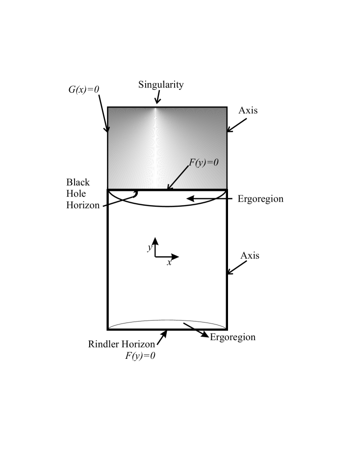
Figure 2: A piece of the $x-y$ plane for the Stationary C-metric. The axis, horizons and the ergo-regions are displayed.

Therefore, the picture of a piece of the $x-y$ plane with their interpretation is shown in Figure 2.

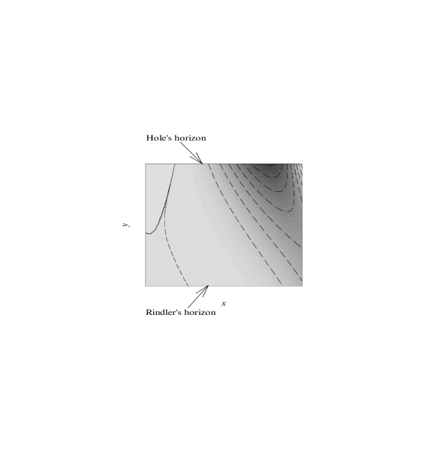
Figure 3: Contour plot of the relative values of the invariant (19) for an outter domain of comunication of the Rotating C-metric (14). The parameters are the following: $w_{1}=-1$, $w_{2}=1$, $w_{3}=2$, $m=1$, $K=1$, $a=1/2$ and $A=1/3$.

The relative value of the invariant (19) is shown in Figure 3. Note its growing values as the singularity is approached.

One last remark. The total mass of the hole as given by

$$\kappa_{(i)}\mathcal{A}_{(i)}^{[k+1,k]}=4\pi\frac{m\left(w_{k+1}-w_{k}\right)}{2}=4\pi\;Mass$$ (26)

now carries information on both acceleration and rotation since the roots depend on those parameters.

Other versions of this solution [25] have similar features.

See the Appendix for the connection between the rotating C metric and the Lewis-Papapetrou coordinates for vacuum stationary axisymmetric spacetimes.

4 Discussions

The C metric can represent several spacetimes depending on the range of the coordinates. As shown in the table I, the spacetimes have singularities, event horizons and conical singularities along the axis. If one takes appropriate combinations of the rectangles in the table I, one gets one of the interpretations found in the literature by some coordinate transformation.

By studying the geometrical quantities of the C metric we find the correct interpretation for the spacetime it generates independently of a particular transformation of coordinates.

This know-how can be of valuable help in the study of black hole accelerated during a finite time. Interesting effects like dragging of inertial frame and gravitational radiation are present.

The main conclusions of our study are: In general, the C metric and the rotating C metric represent accelerated black holes with non smooth compact horizon – there is the possibility of toroidal-like black holes. It requires a fine tuning of the constants to get a smooth compact horizon. In general the axis of symmetry is not elementary flat. The surface gravity at the holes are stronger than the frame acceleration. Therefore the accelerated black hole temperature is higher than the temperature of the thermal bath associated to the accelerated frame. The mass of the black hole can be computed from the mechanics of black holes and it is the asymptotic mass of the Weyl solution of a rod with line density $1/2$. We found no mathematical limitation on the acceleration parameter. For the rotating case the mass has the contribution of the rotation and the acceleration, as it should.

Although the solutions have some bizarre features, they give us lots of informations on how the spacetime is dragged along an accelerated black hole. The extension of uniqueness theorems to include accelerating black holes is investigated in [41]

Acknowledgments

We want to thank FAPESP for financial support, also PSL is grateful to CNPq for a research grant and to G. Gibbons for some early conversations about different aspects for the C-metric.

5 Appendix

5.1 C metric and Weyl coordinates

One can improve our interpretation of the C metric through the transformation from the coordinate $(t,x,y,\phi)$ into static axisymmetric spacetime in Weyl like dimensionless coordinates $(t,r,z,\phi)$. This transformation is valid only on the static regions of the $x-y$ plane (the even labeled regions of Table I). Let the Weyl metric be

$$ds^{2}=m^{2}\left[\exp\left(2\psi\right)dt^{2}-\exp\left(2\nu-2\psi\right)\left[dr^{2}+dz^{2}\right]-r^{2}\exp\left(-2\psi\right)d\phi^{2}\right]$$ (27)

$m$ is the dimensional constant which settles the physical scale. The functions $\psi$ and $\nu$ depend only on $r$ and $z$. From (27) and (1) one finds

$$\left.\begin{array}[c]{c}\exp\left(2\psi\right)=\frac{K^{2}F(y)}{\left(mA\right)^{2}\left(x+y\right)^{2}}\\ r^{2}\exp\left(-2\psi\right)=\frac{G(x)}{\left(KmA\right)^{2}\left(x+y\right)^{2}}\end{array}\right\} \Rightarrow r^{2}=\frac{F(y)G(x)}{\left[mA\left(x+y\right)\right]^{4}}$$ (30)

$$\exp\left(2\nu\right)\left[dr^{2}+dz^{2}\right] =\frac{K^{2}F(y)}{\left(mA\right)^{2}\left(x+y\right)^{4}}\left[\frac{dy^{2}}{F(y)}+\frac{dx^{2}}{G(x)}\right]$$

One sees that the roots of $F(y)$ are linked to the regions, in Weyl coordinates, where $\psi\rightarrow-\infty$ . Recall that the Einstein vacuum equations for the Weyl metric (27) reduce to

$$\nabla^{2}\psi \equiv\psi_{rr}+\frac{1}{r}\psi_{r}+\psi_{zz}=0$$

$$d\nu =r\left(\psi_{r}^{2}-\psi_{z}^{2}\right)\;dr+2r\psi_{r}\psi_{z}\;dz$$

Thus the function $\psi$ must be a solution of Laplace’s equation arising from sources lying on the axis $r=0$ [22] and asymptotically behaves as the Newtonian gravitational potential of those sources. Neglecting the negative mass density cases one can show that the Newtonian sources for the even labeled regions of the C-metric have mass density given by [22]

$$\lim_{r\rightarrow 0}\left(\frac{1}{2}r\psi_{r}\right)=\lim_{y\rightarrow w_{i};dx=0}\frac{1}{2}\left(\frac{F_{y}/F-2/(x+y)}{F_{y}/F-4/(x+y)}\right)=\frac{1}{2}$$

It is known that semi-infinite line source and finite line source with mass density $\frac{1}{2}$ are associated, through the Weyl solutions, to Rindler and Schwarzschild spacetimes respectively [32] [20]. Thus, if the cubic (2) has three distinct real roots, the roots of $F$ will be associated to the line sources and the roots of $G$ will be associated to pieces of the $z$-axis. We can assign the points $z_{i}$ along the $z$-axis in Weyl coordinates where the line sources begin or end in such a way that $z_{i}=w_{i}$ so that $z_{i}$ are also the roots of the cubic $Q$.

The conical singularity in Weyl coordinate appears where

$$\lim_{\varepsilon\rightarrow 0}\frac{\int_{0}^{2\pi}r\exp\left(-\psi\right)d\phi}{2\pi\int_{0}^{\varepsilon}\exp\left(\nu-\psi\right)dr}=1/\exp\nu(0,z)$$ (31)

is not unity and the compression force on it is given by[24]

$$F_{z}=\frac{1}{4}\left[\exp\left(-\nu(0,z)\right)-1\right]=\frac{1}{4}\left[\frac{G_{x}\left(-w_{i}\right)}{2K}-1\right]$$ (32)

where the second equality is obtained by the comparison of (11) and (31)

5.2 Rotating C metric and Lewis-Papapetrou coordinates

One can improve our interpretation of the rotating C metric by the comparison of the coordinate system $(t,x,y,\phi)$ with the stationary axisymmetric spacetime in Lewis-Papapetrou coordinates $(t,r,z,\phi)$. This comparison holds only on the stationary regions. Let the metric be

$$ds^{2}=m^{2}\left[\exp\left(2\psi\right)\left(dt-\varpi d\phi\right)^{2}-\exp\left(2\nu-2\psi\right)\left[dr^{2}+dz^{2}\right]-r^{2}\exp\left(-2\psi\right)d\phi^{2}\right]$$ (33)

The functions $\psi$ and $\nu$ and $\varpi$ depend on $r$ and $z$ only and all quantities but $m$ are dimensionless. From (33) and (14) one finds

$$\left.\begin{array}[c]{c}\exp\left(2\psi\right)=\frac{K^{2}W^{-1}}{\left(mA\right)^{2}\left(x+y\right)^{2}}\left[F(y)-\left(aAy^{2}\right)^{2}G(x)\right]\\ r^{2}\exp\left(-2\psi\right)+\varpi^{2}\exp\left(2\psi\right)=\frac{G(x)-\left(aAy^{2}\right)^{2}F(y)}{\left(KmA\right)^{2}\left(x+y\right)^{2}W}\\ \varpi\exp\left(2\psi\right)=\frac{aW^{-1}}{Am^{2}\left(x+y\right)^{2}}\left[x^{2}F(y)+y^{2}G(x)\right]\end{array}\right\}$$ (37)

$$r^{2} =\frac{F(y)G(x)}{\left[mA\left(x+y\right)\right]^{4}}-\left(\frac{a}{m}\right)^{2}\frac{\left[1+\left(mA\right)^{2}\right]\left[x^{2}F(y)+y^{2}G(x)\right]^{2}}{W^{2}\left[mA\left(x+y\right)\right]^{4}}$$ (38)

One sees that the roots of $F(y)-\left(aAy^{2}\right)^{2}G(x)$, the infinite red-shift surfaces, are linked to the regions where $\psi\rightarrow-\infty$ . The full transformation is very complicate and not clarifying. The Einstein vacuum equations for the metric (33) can be written as

$$\nabla^{2}\psi \equiv\psi_{rr}+\frac{1}{r}\psi_{r}+\psi_{zz}=-\frac{\exp\left(4\psi\right)}{2r^{2}}\left(\nabla\varpi\right)^{2}$$

$$\nu_{r} =r\left(\psi_{r}^{2}-\psi_{z}^{2}+\frac{\exp\left(4\psi\right)}{4r^{2}}\left(\varpi_{z}^{2}-\varpi_{r}^{2}\right)\right)$$

$$\nu_{z} =2r\left(\psi_{r}\psi_{z}-\frac{\exp\left(4\psi\right)}{4r^{2}}\varpi_{z}\varpi_{r}\right)$$

$$0 =\nabla\cdot\left(\frac{\exp\left(4\psi\right)}{r}\nabla\varpi\right)$$

where $\nabla$ stands for the flat vector operator $\left(\partial_{r},\partial_{z}\right)$. Thus the function $\psi$ must be a solution of the non-linear Poisson’s equation which have as the source a contribution from the rotation potential $\varpi$. The connection between the solutions of the equations above and the rotating C-metric solution is not simple. Nevertheless it is known that there are soliton solutions associated to Newtonian images of semi-infinite line plus a finite line with mass density $\frac{1}{2}$ that represent the rotating version of the Weyl C-metric [39].

References

- [1] M. Heusler, Black Hole Uniqueness Theorems. Cambridge University Press, Cambridge (1996).
- [2] R. Geroch and J.B. Hartle, “Distorted black holes”, J. Math. Phys. 23, 680-692 (1982)
- [3] S. Chandrasekhar, The Mathematical Theory of Black Holes. Claredon Press, Oxford (1983).
-
[4]
M. Rees, “Astrophysical evidence of black holes” in R. Wald
(Ed), Black Holes and Relativistic Stars. The University of Chicago
Press, Chicago (1998).
Ibdem, astro-ph/9701161. - [5] A. Abrahams, D. Bernstein, D. Hobill, E. Seidel and L. Smarr, “Numerically generated black-hole spacetimes: Interaction with gravitational waves”, Phys. Rev. D 45, 3544-3558 (1992).
-
[6]
S.W. Hawking and R. Penrose, “The singularities of
gravitational collapse and Cosmology”, Proc. Royal Soc. of London
A314, 529 (1970).
R. Wald, “Gravitational collapse and cosmic censorship”, gr-qc/9710068. - [7] K.S. Thorne, “Nonspherical gravitational collapse – A short review”, in J.R. Klauder (Ed.), Magic without magic: John Archibald Wheeler, H. Freeman, San Francisco, p 231 (1972).
- [8] W. Israel, “Dark stars: The evolution of an idea”, in S.W. Hawking and W. Israel (Eds.) 300 years of Gravitation, Cambridge University Press, Cambridge, p 199 (1987).
-
[9]
G. Galloway, “On the topology of black holes”
Commun. Math. Phys. 151, 53-66 (1993).
J.P.S. Lemos, “Two-dimensional black holes and planar general relativity”, Class. Quantum Gravity 12, 1081 (1995).
C.S. Peça and J.P.S. Lemos, “Thermodynamics of toroidal black holes”, gr-qc/9808035. -
[10]
J.D. Bekenstein, “Black holes and entropy”
Physics Today January 24 (1980).
J.D. Bekenstein, “Black holes and entropy”, Phys. Rev. D 7, 2333 (1973). - [11] R. Wald (Ed), Black Holes and Relativistic Stars. The University of Chicago Press, Chicago (1998). Part II.
-
[12]
A. Strominger and C. Vafa, “Microscopic origin of the
Bekenstein-Hawking entropy” Phys. Lett. B379 99
(1996).
J. Maldacena and A. Strominger, “Black hole greybody factor and D-brane spectroscopy”, Phys. Rev. D 55 861 (1997). -
[13]
F. Dowker, J. Gaunltlett, S. Giddings and G. Horowitz,
“Pair creation of extremal black holes and Kaluza-Klein monopoles”,
Phys. Rev. D 50, 2662-2679 (1994).
I.S. Booth and R.B. Mann, “Cosmological pair production of charged and rotating black holes”, gr-qc/9806051 (1998).
R.B. Mann, “Pair production of topological anti-de Sitter black holes”, Class. Quantum Gravity 14, L109-L114 (1997). - [14] T Levi-Civita, Atti Accel. dei-Lincei, Rendiconti. 27, 343 (1918).
- [15] H. Weyl, “Bemerkung über die axisymmetrishen Lösungen der Einsteinschen Gravitationsgleichungen” Ann. d. Physik 59, 185 (1919).
- [16] W. Kinnersley and M. Walker, “Uniformly accelerating charged mass in general relativity”, Phys. Rev. D 2, 1359-1370 (1970).
- [17] J.F. Plebanski and M. Demianski, “Rotating, charged and uniformly accelerating mass in general relativity”, Annals of Phys. 98, 98-127 (1976).
- [18] J. Bičák and B. Schmidt, “Asymptotically flat radiative spacetimes with boost-rotation symmetry: the general structure”, Phys. Rev. D 40, 1827-1853 (1989).
-
[19]
J. Bičák, “Selected solutions of Einstein’s field
equations: their role in general relativity and astrophysics”,
gr-qc/0004016.
J. Bičák, “Exact radiative spacetimes: some recent developments”, Annalen Phys. 9, 207-216 (2000). -
[20]
W.B. Bonnor, “The sources of the Vacuum C-Metric”,
GRG 15, 535-551 (1983).
W.B. Bonnor, “The C-metric with , ”, GRG 16, 269-281 (1984).
W. Yongcheng, “Vacuum C metric and the metric of two superposed Schwarzschild black holes”, Phys. Rev. D 55, 7977-7979 (1997). - [21] H. Farhoosh and R.L. Zimmerman, “Killing horinzons and dragging of the inertial frame about a uniformly accelerating particle”, Phys. Rev. D 21, 317-327 (1980).
- [22] F.H.J. Cornish and W.J. Uttley, “The interpretation of the C Metric. The Vacuum case”, GRG, 27, 439-454 (1995).
-
[23]
H. Farhoosh and R.L. Zimmerman, “Stationary
charged C-metric”, J. Math. Phys. 20, 2272-2279
(1979).
F.H.J. Cornish and W.J. Uttley, “The interpretation of the C-metric – the charged case when ”, GRG 27, 735-749 (1995). -
[24]
P.S. Letelier and S.R. Oliveira, “Superposition
of Weyl solutions: the equilibrium forces”, Class. Quantum Grav.,
15, 421-433 (1998).
P.S. Letelier and S.R. Oliveira, “Double Kerr-NUT spacetimes: spinning strings and spinning rods”, Phys. Lett. A 238, 101-106 (1998). - [25] H. Farhoosh and R.L. Zimmerman, “Killing horinzons around a uniformly accelerating and rotating particle”, Phys. Rev. D 22, 797-801 (1980).
- [26] A. Tomimatsu, “Power-law tail of gravitational waves from a uniformly accelerating black hole”, Phys. Rev. D 57, 2613-2616 (1998).
- [27] E.T. Newman and L. Tamburino, J. Math. Phys, 2, 667 (1961).
- [28] D. Kramer, H. Stephani, E. Herlt, and M. MacCallum, E. Schmutzer (Ed.) Exact Solutions of Einstein’s field equations, Cambridge University, Cambridge (1980).
- [29] J. Carminati and R.G. McLenaghan, “Algebraic invariants of the Riemann tensor in a four-dimensional Lorentzian space. J. Math. Phys. 32, 3135-3140 (1991).
- [30] P. Musgrave, D. Pollney, K. Lake, Grtensor II software, available from: http://astro.queensu.ca/~grtensor/ (1998).
-
[31]
M.P. do Carmo, Elements of Differential Geometry,
Prentice-Hall, Rio de Janeiro (1974). Apendix 1
S. Kobayashi and K. Nomizu, Foundations of Differential Geometry, vol I, Interscience, Newy York (1963). - [32] H. Bondi, “Negative mass in general relativity”, Reviews of Modern Physics, 29, 423-428 (1957).
- [33] H. Curzon. “Cylindrical solutions of Einstein’s gravitation equations”, Proc. London Math. Soc. 23, 477-480 (1924).
- [34] W. B. Bonnor and N. S. Swaminarayan, “An exact solution for uniformly accelerated particles in general relativity”, Zeitschrift für Physik 177, 240-256 (1964).
- [35] Z. Zheng, J.H. Zhank and Y.L. Jiang, “A jet appearing when a black hole event horizon touches the Rindler horizon”, Int. J. Theor. Phys. 36, 1359-1368 (1997)
-
[36]
P.J. Yi “Vanishing Hawking radiation from a uniformly
accelerated black hole”, Phys. Rev. Lett. 75, 382
(1995).
S. Massar and R. Parentani, “Vanishing Hawking radiation from a uniformly accelerated black hole - Comment”, Phys. Rev. Lett. 78 4526 (1997).
M.C. Sun, Z. Ren, Z. Zheng, “Hawking effect of a rotating, arbitrarily accelerating black hole”, Nuovo Cimento B 110, 829-837 (1995) - [37] B.B. Godfrey, “Horizons in Weyl metrics exhibiting extra symmetries”, GRG 3, 3-16 (1972).
- [38] J. Bičák and V. Pravda, “Spinning C metric: radiative spacetime with accelerating, rotating black holes”, Phys. Rev. D 60, 044004 (1999).
- [39] P.S. Letelier, “Static and stationary multiple soliton solutions to the Einstein equations”, J. Math. Phys. 26, 467-476 (1985).
- [40] F.J. Ernst, “Generalized C-metric”, J. Math. Phys. 19, 1986-1987 (1978).
- [41] C. G. Wells, “Extending the black hole uniqueness theorems I. Accelerating black holes: The Ernst solution and C-metric”, gr-qc/9808044.