Singularity deep inside the spherical charged black hole core

Abstract

We study analytically the spacelike singularity inside a spherically-symmetric, charged black hole coupled to a self-gravitating spherical massless scalar field. We assume spatial homogeneity, and find a generic solution in terms of a formal series expansion. This solution is tested against fully-nonlinear and inhomogeneous numerical simulations. We find full compliance between our analytical solution and the pointwise behavior of the singularity in the numerical simulations. This is a strong scalar-curvature monotonic spacelike singularity, which connects to a weak null singularity at asymptotically-late advanced time.

PACS number(s): 04.70.Bw, 04.20.Dw

]

I Introduction

The spacetime singularities, which classical General Relativity (GR) predicts under very plausible assumptions to inevitably occur inside black holes [1], are a major challenge for Physics, as the currently known physical laws are presumably invalid at such singularities. Instead, some other theory, as yet unknown, is expected to take over and control their structure. However, the GR predictions are still of the greatest importance, as they reveal the spacetime structure under extreme conditions in the strong-field regime.

In the last few years, much advance in the study of black hole singularities has been achieved in the framework of classical GR. Poisson and Israel showed that when non-linear perturbations were allowed, the inner horizon of Reissner-Nordström evolved into a scalar curvature singularity, where the internal mass function diverged and curvature blew up [2]. For spinning or charged black holes, it has been found that at least for a portion of the singularity the latter is null and weak [3, 4]. Namely, despite the divergence of spacetime curvature at the singularity, its tidal influence on extended physical objects is bounded. The detailed structure of the null weak singularity was studied numerically [5, 6] and analytically [7, 8] in the context of a spherical charged black hole, non-linearly perturbed by a self-gravitating, minimally-coupled, massless scalar field. (In the case of a spinning black hole, the evidence for the occurrence of the null weak singularity emerged from analytical perturbative [4] and non-perturbative [9] analyses.) It has been found numerically [5, 6], that under the impact of the non-linear scalar field, the generators of the Cauchy horizon are monotonically focused, until the focosing effect is complete, and the singularity becomes spacelike, rather than null.

Although the existence of a spacelike singularity was suggested by several independent numerical simulations [10, 5, 6], that spacelike singularity has not been shown analytically to exist: its very occurrence is a non-linear effect, and no fully non-linear analytical analyses of the problem have been performed. In addition, the properties of that singularity (both geometrical and physical) have not been studied in detail. In fact, the occurrence suggested by the numerical simulations is the only thing currently known about the spacelike singularity inside charged black holes. It is the purpose of this paper to study the spacelike singularity in the model of a spherical charged black hole and a neutral massless scalar field (the same model for which the singularity was found numerically).

The organization of the paper is as follows. In Section II we show that within a simplified homogeneous model one indeed finds a generic solution describing a spacelike singularity. This model is used to analyze the behavior of geometry and the scalar field near the singularity. In Section III we describe fully-nonlinear and inhomogeneous numerical simulations which test the validity of the homogeneity assumption of our analytical model. We find full compliance between the analytical results and the pointwise behavior found in the numerical simulations. We also use the numerical simulations to study the spatial structure of the singularity. We conclude and discuss our results in Section IV.

II Analytical homogeneous model

In order to facilitate the analysis, we make the simplifying assumption, that the singularity can be modeled to be homogeneous. (This assumption is justified a posteriori numerically.) That is, we assume that spatial gradients of the dynamical fields are negligible near the spacelike singularity compared with temporal gradients. Consequently, our analysis can actually probe just the pointwise behavior at the singularity. The spatial dependence, however, cannot be studied with this model. We shall therefore study the spatial dependence numerically below in Sec. III.

We write the general homogeneous spherically-symmetric line element as

$$\,ds^{2}=h(r)\,dt^{2}+f(r)\,dr^{2}+r^{2}\,d\Omega^{2}$$ (1)

where $\,d\Omega^{2}=\,d\theta^{2}+\sin^{2}\theta\,d\phi^{2}$ is the metric on the unit two-sphere. Here, $r$ is the radial coordinate, defined such that spheres of radius $r$ have surface area $4\pi r^{2}$ (note that $r$ is timelike inside the black hole), and $t$ is normal to $r$ ($t$ is spacelike inside the black hole. There is a gauge freedom in $t$—see below). The Einstein-Maxwell-scalar equations (with a free electric field corresponding to charge $q$ and with a scalar field $\Phi$) are then given by

$$\left(f^{\prime}r+f^{2}-f\right)/\left(fr^{2}\right)=\Phi^{\prime 2}+f\,q^{2}/r^{4}$$ (2)

$$\left(h^{\prime}r-hf+h\right)/\left(hr^{2}\right)=\Phi^{\prime 2}-fq^{2}/r^{4}$$ (3)

$$\left[\left(h^{2}\right)^{\prime}\,\left(f-\frac{1}{2}rf^{\prime}\right)+2rf\,\left(hh^{\prime\prime}-\frac{1}{2}h^{\prime 2}\right)-2f^{\prime}h^{2}\right]$$ (4)

$$/\left(4rfh^{2}\right)=fq^{2}/r^{4}-\Phi^{\prime 2}$$ (5)

in addition to the Klein-Gordon equation $\nabla^{\mu}\nabla_{\mu}\;\Phi=0$, whose first integral is $\Phi^{\prime}(r)=d\;\sqrt{|f/\left(hr^{4}\right)|}$, where $d\neq 0$ is an integration constant. Here, a prime denotes differentiation with respect to $r$, and $\nabla_{\mu}$ denotes covariant differentiation. We seek a generic solution to these equations describing a spacelike singularity at $r=0$.

The source terms for the field equations [the right-hand side (RHS) of Eqs. (2)–(5)] contain contributions from both the electric field and the scalar field. We find that for a dominant electric-field contribution near the singularity at $r=0$, the latter is timelike, rather than spacelike. As in this case the scalar field’s contribution to the field equations is negligible compared with the electric field’s contribution near $r=0$, to the leading order in $r$ one would expect to find the same solution as with no scalar field at all. However, from the generalized Birkhoff theorem the solution in the latter case is nothing but the Reissner-Nordström solution. Namely, with dominant electric field, to the leading order in $r$ the singularity is indistinguishable from the Reissner-Nordström singularity, which is timelike. We note in passing that this case might be of some relevance for consideration of the self-gravitating scalar field for a hypothetical extension of the spacetime manifold beyond the weakly singular Cauchy horizon. A second case is scalar field and electric field which are comparable in strength near $r=0$. It turns out that there is no consistent solution for comparable electric- and scalar-field contributions at the singularity. The third case is the case where the electric field’s contribution to the energy-momentum tensor near the singularity is negligible compared with the scalar field’s contribution, and to this case we shall specialize below. We emphasize that the causal structure of the singularity at $r=0$ depends on which field dominates: if the electric field dominates the singularity is timelike, and if the scalar field dominates the singularity is spacelike. Note, that in this sense the spacelike singularity we are studying is similar to the spacelike singularity with vanishing charge. In fact, we find that to the leading order in $r$ the singularity in our case is indistinguishable from the singularity in the uncharged case. However, in our case the spacelike singularity is a non-linear effect, whereas in the uncharged case a spacelike singularity exists even with a vanishing scalar field (the Schwarzschild singularity). (There are additional differences between the spacelike singularities in the two cases [11].) Another comment to be made about the timelike singularity is that it is reasonable to expect a linear perturbation analysis to be valid near it, as the non-linear effects of the scalar field are negligible.

We assume a formal series expansion for the metric functions of the general form $f^{(n)}(r)=\sum_{i=1}^{n}f_{i}(r)$ and $h^{(n)}(r)=\sum_{i=1}^{n}h_{i}(r)$, and assume that both series have a finite radius of absolute convergence to $f$ and $h$, respectively, in the limit $n\to\infty$. We also assume that for all values of $i$, $f_{i}(r)=f_{i0}\,r^{m_{i}}$ and $h_{i}(r)=h_{i0}\,r^{n_{i}}$, with constant $f_{i0}$ and $h_{i0}$. (These assumptions are justified a posteriori numerically.) We then find the leading terms in $r$ for the metric functions, namely

$$f(r) = -(\beta+1)C\,r^{\beta+2}$$ (6)

$$+ \frac{(\beta+1)^{2}(3\beta+2)}{\beta^{2}}\;C^{2}\;q^{2}\;r^{2\beta+2}+O(r^{2\beta+2+\gamma})$$ (7)

$$h(r)=d^{2}C\;r^{\beta}-d^{2}\frac{(\beta+1)(\beta+2)}{\beta^{2}}\;C^{2}\;q^{2}\;r^{2\beta}+O(r^{2\beta+\gamma})$$ (8)

where $C$ and $\beta$ are positive parameters. Here, $\gamma=2$ if $\beta>2$ and $\gamma=\beta$ otherwise. For the scalar field we find

$$\Phi(r) = \sqrt{\beta+1}\;\ln r-\frac{(\beta+1)^{3/2}(3\beta+2)}{2\beta^{3}}\;C^{2}\;q^{2}\;r^{\beta}$$ (9)

$$+ O(r^{\beta+\gamma}).$$ (10)

This form for the solution suggests that $f,h$ are given by infinite double series

$$f,h=\sum_{m=1}^{\infty}\sum_{n=1}^{\infty}a_{mn}^{f,h}\;r^{\beta m+(\beta+2)(n-1)+\sigma_{f,h}},$$ (11)

$a_{mn}^{f}=a_{mn}^{f}(C,\beta)$ and $a_{mn}^{h}=d^{2}\tilde{a}_{mn}^{h}(C,\beta)$ being the expansion coefficients. Here, $\sigma_{f}=0$ and $\sigma_{h}=-2$. As we have already remarked, the black hole electric charge does not appear in the leading order terms of either the metric functions or the scalar field. This is a direct consequence of the dominance of the scalar field over the electric field near the singularity. Consequently, the derivation of the solution is similar to the derivation in [11], and further details can be found there. The charge affects the spacetime geometry and the behavior of the scalar field in higher order terms, however, as is evident from the solution, such that at any finite value of $r$, even very close to the singularity, both the geometry and the field are different from the uncharged case’s counterparts. Note, that we find the parameter $\beta$ to be positive. In the case of the spacelike singularity inside an uncharged black hole, the corresponding parameter is found to be greater than $-1$, which is the value found for the Schwarzschild singularity. Thus, in the uncharged case the parameter $\beta$ changes continuously from its vacuum value, whereas in the charged case we study here it jumps discontinuously from the $-2$ value of the Reissner-Nordström singularity which corresponds to the (electro-)vacuum limit of our spacetime, to positive values. This discontinuity is the result of the non-linear nature of the spacelike singularity: with no scalar field (the electro-vacuum case) the singularity at $r=0$ is timelike. With the addition of a scalar field the only singularity we find is spacelike. The change from timelike to spacelike is discontinuous, and this is what we indeed find.

From this solution, we draw the following inferences: First, we define a ‘tortoise’ coordinate $r_{*}$ by $g_{r_{*}r_{*}}=-g_{tt}$. Then, null coordinates are defined by $t=(v-u)/2$ and $r_{*}=(v+u)/2$, with ingoing $v$ and outgoing $u$. For a certain outgoing ray $u=u_{0}\equiv\rm{const}$ which runs into the spacelike singularity, the latter is hit at some finite value of advanced time $v=v_{*}$ (see Fig. 1). (The null singularity is located at $v=\infty$.) We find that to the leading order in $v_{*}-v$

$$r(u_{0},v)=\left[d^{2}/(\beta+1)\right]^{1/4}\;(v_{*}-v)^{1/2}.$$ (12)

This property of the spacelike singularity inside a non-linearly perturbed charged black hole is similar to the properties of the singularity inside uncharged black holes [11]. We next consider an observer who follows a radial $t={\rm const}$ trajectory. Let $\tau$ be that observer’s proper time, set such that $\tau=0$ at $r=0$. We denote by $x^{0}$ the coordinate tangent to the worldline. Then, to the leading order in $\tau$, the $(00)$ tetrad component of the Ricci tensor and the Kretschmann scalar, correspondingly, are given by

$$R_{(0)(0)}(\tau)=8\;\frac{\beta+1}{(\beta+4)^{2}}\;\frac{1}{\tau^{2}}$$ (13)

$$R_{\alpha\beta\gamma\delta}R^{\alpha\beta\gamma\delta}(\tau)=64\;\frac{2\beta(\beta+1)+3}{(\beta+4)^{4}}\;\frac{1}{\tau^{4}}.$$ (14)

As Eqs. (13) and (14) are given to the leading order in $\tau$, they are identical to the corresponding equations in the uncharged case (cf. [11]). Equation (14) implies that this is a scalar-curvature singularity. From Eq. (13) and from the theorem by Clarke and Królak [13] it then follows that this singularity is strong in the Tipler sense [14], as the twice integrated $R_{(0)(0)}(\tau)$ over $\tau$ diverges logarithmically as $\tau\to 0$. Namely, any extended physical object will unavoidably be crushed to zero volume upon arrival to the singularity. As we find that $\beta>0$, we infer that there is no finite $\beta$ which nullifies any of the RHS’s of either Eq. (13) or Eq. (14). Consequently, for the entire range of permissible parameters, this is a strong scalar-curvature singularity. This property of the singularity is in sharp contrast with the Cauchy horizon singularity, which is known to be null and weak.

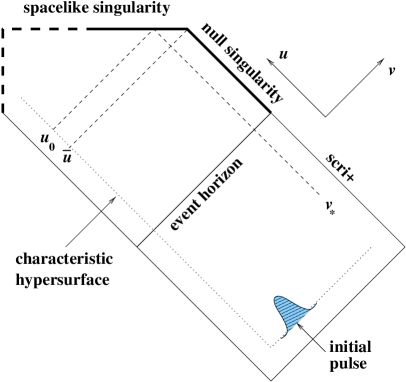
FIG. 1.: The Penrose diagram of the simulated spacetime. Singularities are depicted by thick lines. Dashed thick lines denote regions of the singularity not covered by the domain of integration, and describe a possible picture of these portions. The causal structure of the singularity changes from null to spacelike at $(u=\bar{u},v=\infty)$. For any outgoing null ray at $u=u_{0}>\bar{u}$ the spacelike singularity is reached at $v=v_{*}$.

Let us consider the genericity of our solution. The notion of a general solution for non-linear differential equations is not unambiguous. However, we can count the number of arbitrary parameters in our solution, and thus show that it is generic. From the physical point of view, one would expect two arbitrary parameters (one because of Birkhoff’s theorem and one due to the scalar field. Note that as the scalar field is neutral, the electric charge is fixed). Apparently, our solution has three arbitrary parameter, namely $\beta$, $d^{2}$, and $C$. However, the arbitrariness in $d^{2}$ reflects merely a trivial gauge mode, i.e., the freedom to re-scale the coordinate $t$ (see Ref. [11]). Consequently, our solution has two physical degrees of freedom, and is therefore generic. These considerations do not rule out the possible existence of other generic solutions. However, this solution is the one which is realized in the numerical simulations (see below).

III Fully inhomogeneous numerical simulations

The analytical approach presented above assumes the singularity to be homogeneous. However, the spacetime inside black holes (even very close to the singularity) is expected in general to be inhomogeneous. To what extent then is the homogeneity assumption restrictive? We shall present in what follows the results of fully non-linear and inhomogeneous numerical simulations. We show, that the above homogeneous analytical model succeeds to describe the pointwise behavior of the singularity as inferred from the inhomogeneous simulations. In this sense the assumption of homogeneity is a simplification which does not ruin the structure of the singularity, as the numerical simulations reveal that the dependence of the geometry at and near the singularity depends only weakly on spatial coordinates: it is the temporal gradients which dominate. However, the spatial dependence can still be studied numerically. We shall do just this after we confront the predictions of the analytical model with the pointwise behavior of the numerical simulations.

Let us discuss then the results obtained from fully non-linear (and inhomogeneous) numerical simulations. We used the same code which was used in Ref. [6] (see also [15]) to study the null singularity in this model. This code is based on double-null coordinates and on free evolution of the metric functions and fields. The code is stable and converges with second order. (Slight adaptations of the code were needed, to allow for a careful approach to $r=0$. These modifications are described in Ref. [11].) Our initial value set-up is such that prior to the smooth initial pulse of compact support the geometry is Reissner-Nordström with charge $q$ and mass $M$ (see Fig. 1). Then, due to the scalar field the geometry is changed, and the final mass of the black hole is $M_{f}$.

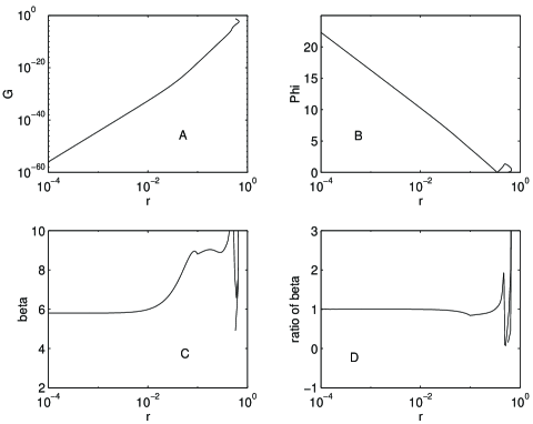
FIG. 2.: (A) The metric function $G=-2g_{uv}$. (B) The scalar field $\Phi$. (C) The parameter $\beta$ as calculated from the exponent of $h$. (D) The ratio of $\beta$ as calculated from the exponent of $h$ and $\beta$ as calculated from the amplitude of $\Phi$. In all graphs the abscissae are $r$.

Figures 2, 3 and 4 display the results of the numerical simulations with $q/M=0.998$ and $M_{f}/M\approx 1.51$. We have also performed numerical simulations with other values of the parameters, and found no qualitative change of the behavior. In fact, when we increase the amplitude of the scalar-field pulse (while keeping the support of the pulse fixed), we find the following two effects. First, the ratio $M_{f}/M$ increases, as should be expected from the greater energy content of the pulse. Second, the larger the amplitude, the earlier the spacelike singularity occurs. Namely, with larger amplitude for the initial pulse the generators of the Cauchy horizon focus faster, and the Cauchy horizon focuses completely within a smaller lapse of affine parameter. However, the spacelike singularity itself is unchanged by this change of the initial parameters, and is in this sense robust. Very similarly, varying the value of $q/M$ does not change the properties of the singularity. This should indeed be expected from our analytical considerations of Section II: the singularity is dominated by the scalar field, and to the leading order in $r$ the charge of the black hole has no effect.

The data are shown along an outgoing ray at $u_{0}$ approaching the spacelike singularity at $r=0$ (similar results are obtained for any choice of such an outgoing ray; in all four graphs of Fig. 2 the abscissae are $r$): 2(A) the metric component $g_{uv}$, for double-null coordinates defined such that $v=r$ on the outgoing segment of the characteristic hypersurface, and $u\propto-r$ on its ingoing segment. The vanishing of $g_{uv}$ implies the vanishing of both $f$ and $h$. Moreover, the asymptotically linear curve in this plot implies a power-law behavior near the singularity. (This is checked more accurately in Fig. 2(C).) Figure 2(B) displays the scalar field $\Phi$. We find that $\Phi$ diverges logarithmically, in agreement with Eq. (10). Figure 2(C) shows the local power index of $g_{uv}$, namely, the local slope in Fig. 2(A). The asymptotically constant value to which the local power approaches—in agreement with Eqs. (7) and (8)—implies that the power-law assumption for the metric functions is justified. In fact, this power-law index is just the value of the parameter $\beta$ for the intersection point of the outgoing ray under consideration with the spacelike singularity. Finally, we test another aspect of the analytical model. We found that the same parameter $\beta$ appears in two different contexts, namely, in the exponent of the metric functions [Eqs. (7) and (8)], and in the amplitude of the scalar field [Eq. (10)]. The ratio of these two values for $\beta$ is predicted, therefore, to asymptotically approach a value of unity. This is indeed shown in Fig. 2(D), to within $1$ part in $10^{3}$.

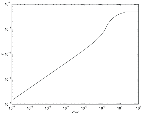
FIG. 3.: The radial coordinate $r(u_{0},v)$ as function of (advanced-time) distance $v_{*}-v$ from the spacelike singularity. The singularity is located at $v=v_{*}$.

Figure 3 shows $r(u_{0},v)$ as a function of the distance (in terms of advanced time) from the singularity $v_{*}-v$. The slope is equal asymptotically to the value of $1/2$ implied by Eq. (12) to within a numerical error of $1\%$.

Finally, we use the numerical simulation in order to check the spatial dependence of the solution. Figure 4 displays the value of the parameter $\beta$ as a function of advanced time, namely, as a function of the value of $v_{*}$ at which the outgoing ray under consideration hits the singularity. We find that along the spacelike singularity, upon approach to the spacetime event where the causal structure of the singularity changes from null to spacelike, $\beta$ increases rapidly. This suggests that at the particular outgoing ray at $u=\bar{u}$ for which that event is reached $\beta$ may be infinite. We can therefore compare the relative strength of different points along the spacelike singularity. Although this singularity is strong throughout, the nearer one is to the spacetime event where the causal structure changes, the weaker is the strong singularity, as curvature scalars diverge slowlier. That is, let us consider a constant $r$ hypersurface near the singularity (namely, deep in the asymptotic region). Then, approaching $\bar{u}$ along this hypersurface curvature scalars decrease (as $\beta$ increases). This fits well with our overall picture: when the singularity first forms it is null and weak. At later times, the weak null singularity becomes stronger with increasing affine parameter. This is manifested by the focusing effect, and by the inverse proportion of the blue-shift factors to the area coordinate [8]. Thus, we have a weak singularity which becomes stronger. Then, at $u=\bar{u}$, $r$ vanishes and the causal structure of the singularity changes and it becomes spacelike and strong, and strengthens as one gets farther from the changing point, namely, as $u-\bar{u}$ increases.

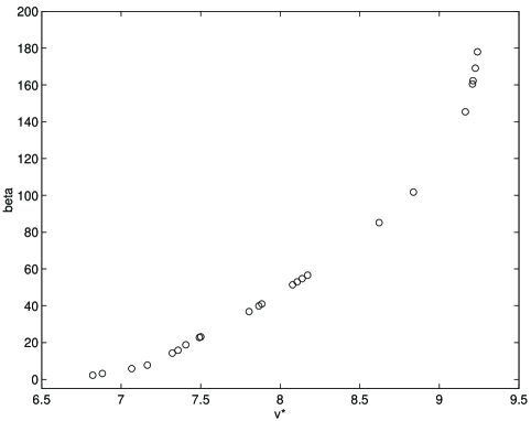
FIG. 4.: The value of $\beta$ for different outgoing null rays as a function of $v_{*}$, namely, as a function of the value of the ingoing coordinate $v$ for which the spacelike singularity is reached when approached along outgoing null rays.

IV Discussion

We find analytically a simple homogeneous model, which describes the pointwise behavior of the spacelike singularity which occurs inside spherical charged black holes with a non-linear scalar field. This singularity is generic in the sense that the solution has the expected number of free parameters. The numerical simulations imply that the singularity we find in the simple homogeneous model successfully describes the pointwise behavior of the singularity of the fully nonlinear and in general inhomogeneous spacetime. The spacelike singularity is scalar curvature (like the null singularity which precedes it), monotonic, and strong (unlike the null singularity, which is weak).

It remains an open question, to what extent this simple model captures the essence of the singularity inside realistic black holes, namely, spinning black holes with vacuum perturbations: First, scalar fields are known to be related to unique phenomena, such as the destruction of the oscillations of the Belinskii-Khalatnikov-Lifshitz (BKL) singularity [16]. Second, we find that the scalar field in our model is dominant near the singularity, whereas the BKL singularity is often dominated by vacuum perturbations rather than by matter fields [17]. Finally, both the spherical symmetry and the scalar field are mere toy models for the more realistic cases. A major open question is then whether in more realistic cases there would indeed be a spacelike singularity to the future of the null singularity, and whether it would be monotonic – like the spacelike singularity inside spherical charged black holes with a scalar field – or oscillatory – like the BKL singularity.

REFERENCES

- [1] S. W. Hawking and G. F. R. Ellis, The large scale structure of space-time, (Cambridge University Press, Cambridge, 1973).
- [2] E. Poisson and W. Israel, Phys. Rev. D 41, 1796 (1990).
- [3] A. Ori, Phys. Rev. Lett. 67, 789 (1991).
- [4] A. Ori, Phys. Rev. Lett. 68, 2117 (1992).
- [5] P. R. Brady and J. D. Smith, Phys. Rev. Lett. 75, 1256 (1995).
- [6] L. M. Burko, Phys. Rev. Lett. 79, 4958 (1997).
- [7] A. Bonanno, S. Droz, W. Israel, and S. M. Morsink, Proc. R. Soc. London A 450, 553 (1995).
- [8] L. M. Burko and A. Ori, Phys. Rev. D 57, R7084 (1998).
- [9] P. R. Brady, S. Droz, and S. M. Morsink, Report No. gr-qc/9805008.
- [10] M. L. Gnedin and N. Y. Gnedin, Class. Quantum Grav. 10, 1083 (1993).
- [11] L. M. Burko, Phys. Rev. D 58, 084013 (1998).
- [12] L. M. Burko, in Internal structure of black holes and spacetime singularities, volume XIII of the Annals of the Israel Physical Society, edited by L. M. Burko and A. Ori (Institute of Physics, Bristol, 1997).
- [13] C. J. S. Clarke and A. Królak, J. Phys. Geom. 2, 127 (1985), proposition 5.
- [14] F. J. Tipler, Phys. Lett. A 64, 8 (1977).
- [15] L. M. Burko and A. Ori, Phys. Rev. D 56, 7820 (1997).
- [16] V. A. Belinskii and I. M. Khalatnikov, Zh. Eksp. Teor. Fiz. 63, 1121 (1972) [Sov. Phys. JETP 36, 591 (1973)].
- [17] L. D. Landau and E. M. Lifshitz, The Classical Theory of Fields, Fourth Edition (Pergamon, Oxford, 1975).