All nonspherical perturbations of the Choptuik spacetime decay

Abstract

We study the nonspherical linear perturbations of the discretely self-similar and spherically symmetric solution for a self-gravitating scalar field discovered by Choptuik in the context of marginal gravitational collapse. We find that all nonspherical perturbations decay. Therefore critical phenomena at the threshold of gravitational collapse, originally found in spherical symmetry, will extend to (at least slightly) nonspherical initial data.

I Introduction and summary

We have many and powerful results about the static or stationary end-states of gravitational collapse. However, very little is known in comparison about the dynamical evolution towards them. Analytical studies are limited by the complicated non-linear nature of the equations. Numerical studies can fill this gap if they can demonstrate generic behavior.

Starting with the pioneering work of Choptuik [1], a number of authors have shown that, despite the complicated nature of the equations, the threshold of gravitational collapse is strikingly simple [2]. Following the initial ideas of Evans [3] it has been possible to explain this simplicity as the consequence of the existence of a “critical solution” which acts as an intermediate attractor in phase space. This solution has a single linearly-unstable eigenmode which drives out every nearby solution either towards black hole formation or dispersal, leaving flat space behind.

This body of work expands our understanding of the dynamical process of collapse, borrowing concepts and tools from the theory of dynamical systems. The emphasis is shifted to phase space, and within it, to solutions with special stability characteristics:

1. First, we look for global attractors. The Minkowski and Kerr-Newman solutions are the only possible end-states of collapse in the Einstein-scalar-Maxwell system.

2. Then we look for codimension-one attractors, which separate phase space into basins of attraction of the global attractors. These solutions are also very important. For example, the study of the trajectories connecting the codimension-one attractors with the global attractors gives us a qualitative picture of marginal collapse because many different trajectories tend to approach them and arrive at the attractors along them. In this terminology, Choptuik discovered the first codimension-one attractor. For reasons still unknown, many of the codimension-one attractors are self-similar.

3. The long-term objective is the construction of a picture of the unfolding of trajectories in phase space. It would contain all the dynamical information about a given system. Furthermore it is the natural place to accommodate the zoo of special solutions we currently know of, including naked singularities.

In a previous paper [4] we addressed the question of whether the Choptuik solution was a codimension-one solution in the system Einstein-Maxwell-charged scalar field, restricted to spherical symmetry, and obtained an affirmative answer, which has been confirmed in independent work [5]. In this paper we address the same question for the system Einstein-real scalar field, but this time allowing for arbitrary small deviations from spherical symmetry, and we obtain again an affirmative answer. The study of the Einstein-Maxwell-charged scalar field system beyond spherical symmetry will be reported elsewhere.

This result, together with a parallel result on the collapse of a perfect fluid [6], strongly suggests that critical phenomena in gravitational collapse are still present in the absence of spherical symmetry. An equally strong indication that critical phenomena are not restricted to spherical symmetry is provided by numerical work on the critical collapse of axisymmetric vacuum spacetimes [7], which shows universality and scaling similar to that of the spherical scalar field.

The plan of the article is as follows: In section II we give a complete review of the Gerlach and Sengupta [8, 9] formalism of gauge-invariant perturbations around a general spherically symmetric spacetime (which typically contains matter and is time-dependent). In section III we re-express these still general tensor equations of section II in an arbitrary basis to facilitate the study of their causal structure. The equations in this section will be of help in any study of linear perturbations around spherical symmetry for arbitrary matter content, in an arbitrary background coordinate system. In section IV we specialize the formalism to massless scalar field matter. The background solution is briefly reviewed in section V, where we specialize to a particular basis, and choose a coordinate system. In sections VI and VII we split the odd and even linear perturbation equations, respectively, into evolution equations and constraints, and identify free data. Section VIII describes our numerical results in detail. The appendix contains a description of our numerical methods for computing the background and then the perturbations on it.

To summarize our main result here, all non-spherical physical perturbations of Choptuik’s solution decay, and therefore the critical phenomena at the black hole threshold in scalar field collapse — universality, echoing and scaling — are expected to persist for initial data that deviate (slightly) from spherical symmetry. Nevertheless, the $l=2$ even-parity perturbations decay quite slowly, and may become apparent in non-spherical collapse situations.

II Review of Gerlach and Sengupta formalism of gauge-invariant perturbations

In this section we give a brief introduction to the formalism of Gerlach and Sengupta [8, 9] for perturbations around the most general spherically symmetric spacetime. Spacetime is decomposed as $M^{4}=M^{2}\times S^{2}$, where $S^{2}$ is the two-sphere and $M^{2}$ is a two-dimensional manifold with boundary. Tensor indices on $M^{4}$ are Greek letters, tensor indices on $M^{2}$ are upper case Latin letters, and tensor indices on $S^{2}$ are lower case Latin letters. We write the general spherically symmetric metric as

$$g_{\mu\nu}dx^{\mu}dx^{\nu}\equiv g_{AB}(x^{D})dx^{A}dx^{B}+r^{2}(x^{D})\gamma_{ab}(x^{d})dx^{a}dx^{b},$$ (1)

where $g_{AB}$ is a metric and $r$ is a scalar field on $M^{2}$. $\gamma_{ab}$ is the unit Gaussian-curvature metric on $S^{2}$. $r=0$ identifies the center of the spherical symmetry, where each $S^{2}$ degenerates to a point. $r=0$ is the boundary of $M^{2}$. In the same way we decompose the spherically symmetric stress-energy tensor:

$$t_{\mu\nu}dx^{\mu}dx^{\nu}\equiv t_{AB}(x^{D})dx^{A}dx^{B}+Q(x^{D})r^{2}(x^{D})\gamma_{ab}(x^{d})dx^{a}dx^{b}.$$ (2)

For simplifying the field equations, it is useful to introduce a vector and a scalar on $M^{2}$ derived from the scalar $r$:

$$v_{A} \equiv \frac{r_{|A}}{r},$$ (3)

$$V_{0} \equiv -r^{-2}+2{v_{A}}^{|A}+3v_{A}v^{A}.$$ (4)

We distinguish covariant derivatives on $M^{4}$, $M^{2}$ and $S^{2}$:

$$g_{\mu\nu;\lambda}\equiv 0,\ \ \ \ g_{AB|C}\equiv 0,\ \ \ \ \gamma_{ab:c}\equiv 0.$$ (5)

We shall also need the covariantly constant unit antisymmetric tensors with respect to $g_{AB}$ and $g_{ab}$, which we call $\epsilon_{AB}$ and $\epsilon_{ab}$.

The Einstein equations in spherical symmetry are

$$G_{AB}=-2(v_{A|B}+v_{A}v_{B})+g_{AB}V_{0} = 8\pi t_{AB},$$ (6)

$$\frac{1}{2}{G_{a}}^{a}=-{\cal R}+{v_{A}}^{|A}+v_{A}v^{A} = 8\pi Q,$$ (7)

where ${G_{a}}^{a}$ denotes the partial trace over $G_{\mu\nu}$. ${\cal R}\equiv\frac{1}{2}R^{(2)A}_{A}$ is the Gaussian-curvature scalar of $M^{2}$. The four-dimensional Ricci scalar is $R=2({\cal R}-V_{0})$. The conservation equation for the stress-energy tensor in spherical symmetry is

$${t_{AB}}^{|B}+2t_{AB}v^{B}=2Qv_{A}.$$ (8)

As a manifestation of the contracted Bianchi identities, (7) can be obtained as a derivative of equation (6), provided that (8) holds.

Now we introduce an arbitrary (not spherically symmetric) perturbation of this spacetime: $g_{\mu\nu}\to g_{\mu\nu}(x^{D})+h_{\mu\nu}(x^{D},x^{d})$ and again we perform a 2+2 decomposition. Furthermore we decompose the angular ($x^{d}$) dependence into series of tensorial spherical harmonics:

• $Y^{m}_{l}(x^{d})$ are the scalar spherical harmonics,

• the objects ${Y^{m}_{l}}_{:a}$ and ${S^{m}_{l}}_{a}\equiv\epsilon_{a}^{\ b}{Y^{m}_{l}}_{:b}$ form a complete basis of vector harmonics, and

• following Zerilli[11], we use the following basis of symmetric tensor harmonics: $Y^{m}_{l}\gamma_{ab}$, ${Z^{m}_{l}}_{ab}\equiv{Y^{m}_{l}}_{:ab}+\frac{l(l+1)}{2}Y^{m}_{l}\gamma_{ab}$, and ${S^{m}_{l}}_{a:b}+{S^{m}_{l}}_{b:a}$, which is a linear combination of the basis introduced by Regge and Wheeler [12]. For $l=0,1$ there is only one linearly independent tensor, namely $\gamma_{ab}Y^{m}_{l}$, while the other two tensors vanish. Gerlach and Sengupta initially [8] used the Regge-Wheeler basis, but in [9] changed to Zerilli’s basis in order to include the cases $l=0,1$ into a single formalism.

All these spherical harmonics have definite parity under spatial inversion: a spherical harmonic with label $l$ is called even if it has parity $(-1)^{l}$ and odd if its parity is $(-1)^{l+1}$; $Y^{m}_{l}$, ${Y^{m}_{l}}_{:a}$ and ${Z^{m}_{l}}_{ab}$ are even and ${S^{m}_{l}}_{a}$ and ${S^{m}_{l}}_{a:b}+{S^{m}_{l}}_{b:a}$ are odd. (An alternative terminology is polar instead of even, and axial instead of odd.) Even and odd perturbations decouple, and different values of $l$ and $m$ decouple. Furthermore, the perturbation equations do not depend on $m$. In the following we consider one value of $l$ and $m$ at a time, and suppress both the indices $l$ and $m$ and the explicit summation over them. $h_{\mu\nu}$ is decomposed into

$$h_{AB} \equiv {\tilde{h}_{AB}}Y,$$ (9)

$$h_{Ab} \equiv {h_{A}^{{\rm E}}}{Y}_{:b}+{h_{A}^{{\rm O}}}{S}_{b},$$ (10)

$$h_{ab} \equiv r^{2}K\gamma_{ab}Y+r^{2}G{Z}_{ab}+h({S}_{a:b}+{S}_{b:a}).$$ (11)

Note that the left-hand sides are components of a tensor on $M^{4}$. On the right-hand side $\tilde{h}_{AB}$ is a tensor on $M^{2}$, and $Y$ is a scalar on $S^{2}$. Similar remarks apply to the other definitions. In the same way we decompose the perturbation $\Delta t_{\mu\nu}$ into tensorial spherical harmonics:

$$\Delta t_{AB} \equiv {\Delta\tilde{t}_{AB}}Y,$$ (12)

$$\Delta t_{Ab} \equiv {\Delta t_{A}^{{\rm E}}}{Y}_{:b}+{\Delta t_{A}^{{\rm O}}}{S}_{b},$$ (13)

$$\Delta t_{ab} \equiv r^{2}{\Delta t^{3}}\gamma_{ab}Y+{\Delta t^{2}}{Z}_{ab}+{\Delta t}({S}_{a:b}+{S}_{b:a}).$$ (14)

where we use the superindices $2$ and $3$ in order to follow the notation of [9]. (They are just labels, not components of any vector.) Some of the coefficients on the right hand side of these expansions are not defined for $l=0,1$ because the corresponding spherical harmonics vanish. In the following, we always point out which of the general equations continue to hold for $l=0$ and $l=1$ if one sets these coefficients to zero.

Now we define gauge-invariant variables, which do not contain perturbations of the background generated by simple coordinate transformations on this background. With the shorthand

$$p_{A}\equiv h_{A}^{{\rm E}}-\frac{1}{2}r^{2}G_{|A},$$ (15)

a complete set of gauge-invariant metric perturbations is

$$k_{AB} \equiv \tilde{h}_{AB}-(p_{A|B}+p_{B|A}),$$ (16)

$$k_{A} \equiv h_{A}^{{\rm O}}-h_{|A}+2hv_{A},$$ (17)

$$k \equiv K+\frac{l(l+1)}{2}G-2v^{A}p_{A}.$$ (18)

A complete set of gauge-invariant matter perturbations is

$$T_{AB} \equiv \Delta\tilde{t}_{AB}-t_{AB|C}p^{C}-t_{AC}p^{C}_{\ |B}-t_{BC}p^{C}_{\ |A},$$ (19)

$$T_{A} \equiv \Delta t_{A}^{{\rm E}}-t_{AC}p^{C}-\frac{r^{2}}{2}QG_{|A},$$ (20)

$$T^{3} \equiv \Delta t^{3}-\frac{1}{r^{2}}(r^{2}Q)_{|C}p^{C}+\frac{l(l+1)}{2}QG,$$ (21)

$$T^{2} \equiv \Delta t^{2}-r^{2}QG,$$ (22)

$$L_{A} \equiv \Delta t_{A}^{{\rm O}}-Qh_{A},$$ (23)

$$L \equiv \Delta t-Qh.$$ (24)

(These are only partially gauge-invariant for $l=0,1$, and therefore a partial gauge fixing is required in those cases in order to eliminate coordinate transformations from the set of arbitrary perturbations.)

For $l\geq 2$ the metric and matter perturbations in any particular gauge can be obtained by freely choosing values for $G$, $h^{{\rm E}}_{A}$ and $h$ (the gauge in which these all vanish is Regge-Wheeler gauge [12]) and then solving the definitions of the gauge-invariant perturbations for the “naked” perturbations.

The perturbed Einstein equations, expressed only in gauge-invariant perturbations, are

$$l\geq 0:\hskip 398.33858pt\mbox{}$$ (25)

$$(k_{CA|B}+k_{CB|A}-k_{AB|C})v^{C}-g_{AB}(2{k_{CD}}^{|D}-{{k_{D}}^{D}}_{|C})v^{C}$$ (26)

$$-(k_{|A}v_{B}+k_{|B}v_{A}+k_{|AB})+\left(V_{0}+\frac{l(l+1)}{2r^{2}}\right)k_{AB}$$ (27)

$$-g_{AB}\left[{k^{F}}_{F}\frac{l(l+1)}{2r^{2}}+2k_{DF}v^{D|F}+3k_{DF}v^{D}v^{F}-{k_{|F}}^{F}-3k_{|F}v^{F}+\frac{(l-1)(l+2)}{2r^{2}}k\right] = 8\pi T_{AB},$$ (28)

$$\frac{1}{2}\{-{k^{AB}}_{|AB}+{{{k^{A}}_{A}}^{|B}}_{|B}-2{k^{AB}}_{|A}v_{B}+{k^{A}}_{A|B}v^{B}+R^{AB}(k_{AB}-kg_{AB})$$ (29)

$$-\frac{l(l+1)}{2r^{2}}k^{A}_{\ A}+{k_{|A}}^{A}+2k_{|A}v^{A}\} = 8\pi T^{3},$$ (30)

$$l\geq 1:\hskip 199.16928pt\mbox{}$$ (31)

$$\frac{1}{2}({k_{AB}}^{|B}-{k^{B}}_{B|A}+{k^{B}}_{B}v_{A}-k_{|A}) = 8\pi T_{A},$$ (32)

$$-\frac{1}{2r^{2}}\left[r^{4}\left(\frac{k_{A}}{r^{2}}\right)_{|C}-r^{4}\left(\frac{k_{C}}{r^{2}}\right)_{|A}\right]^{|C}+\frac{(l-1)(l+2)}{2r^{2}}k_{A} = 8\pi L_{A},$$ (33)

$$l\geq 2:\hskip 28.45274pt\mbox{}$$ (34)

$$-\frac{1}{2}{k^{A}}_{A} = 8\pi T^{2},$$ (35)

$$\frac{1}{2}{k^{A}}_{|A} = 8\pi L.$$ (36)

$R^{AB}$ in (30) are the $AB$ components of the four-dimensional Ricci tensor. Equations (30) and (36) can be obtained as derivatives of the other equations using the linearized equations of stress-energy conservation, which are

$$l\geq 0:\hskip 170.71652pt\mbox{}$$ (37)

$$\frac{1}{r^{2}}(r^{2}T_{AB})^{|B}-\frac{l(l+1)}{r^{2}}T_{A}-2v_{A}T^{3} = (t_{AB|D}+2t_{AB}v_{D})k^{BD}+Q(k_{|A}-2kv_{A})-t_{AB}k^{|B}$$ (39)

$$+\frac{1}{2}t^{BC}k_{BC|A}-\frac{1}{2}t_{AB}{k_{F}}^{F|B}+t_{AB}{k^{BF}}_{|F},$$

$$l\geq 1:\hskip 170.71652pt\mbox{}$$ (40)

$$\frac{1}{r^{2}}(r^{2}T_{B})^{|B}+T^{3}-\frac{(l-1)(l+2)}{2}\frac{T^{2}}{r^{2}} = \frac{1}{2}k_{AB}t^{AB}+Q\left(k-\frac{1}{2}{k^{A}}_{A}\right),$$ (41)

$$(r^{2}L_{B})^{|B} = (l-1)(l+2)L.$$ (42)

III Perturbation equations for arbitrary matter in an arbitrary orthonormal basis

Both in order to transform tensor equations into sets of scalar equations, and in order to separate evolution equations from constraints, it is desirable to introduce an orthonormal frame in $M^{2}$, namely

$$-u_{A}u^{A}\equiv n_{A}n^{A}\equiv 1,\ \ \ \ u_{A}n^{A}\equiv 0.$$ (43)

In the presence of curvature, this cannot be a coordinate basis:

$$[n,u]^{A}=\mu n^{A}-\nu u^{A},\ \ \ \ \mu\equiv{u^{A}}_{|A},\ \ \ \ \nu\equiv{n^{A}}_{|A}.$$ (44)

We define an associated basis of 2-tensors,

$$g_{AB}=-u_{A}u_{B}+n_{A}n_{B},\ \ \ \ \epsilon_{AB}\equiv n_{A}u_{B}-u_{A}n_{B},$$ (45)

$$p_{AB}\equiv u_{A}u_{B}+n_{A}n_{B},\ \ \ \ q_{AB}\equiv n_{A}u_{B}+u_{A}n_{B}.$$ (46)

and use it to decompose the gauge-invariant metric perturbation:

$$k_{AB}\equiv\eta g_{AB}+\phi p_{AB}+\psi q_{AB}.$$ (47)

We define derivatives along the basis vectors:

$$\dot{f}\equiv u^{A}f_{|A},\ \ \ \ f^{\prime}\equiv n^{A}f_{|A},$$ (48)

and re-express the even-perturbation equations in this basis. We also introduce the notation

$$u^{A}v_{A}\equiv U,\quad n^{A}v_{A}\equiv W,\quad W^{2}-U^{2}=v^{A}v_{A}\equiv v^{2}.$$ (49)

For reference we give the background Einstein equations in frame components:

$$W^{\prime}-\dot{U}+\nu W-\mu U-2U^{2}+2W^{2}-r^{-2} = 8\pi\frac{1}{2}{t_{A}}^{A}\ ,$$ (50)

$$-W^{\prime}-\dot{U}+\nu W+\mu U-U^{2}-W^{2} = 8\pi\frac{1}{2}p_{AB}t^{AB}\ ,$$ (51)

$$-U^{\prime}-\dot{W}+\mu W+\nu U-2UW = 8\pi\frac{1}{2}q_{AB}t^{AB}\ ,$$ (52)

$$-{\cal R}+W^{\prime}-\dot{U}+\nu W-\mu U-U^{2}+W^{2} = 8\pi Q\ .$$ (53)

We use them among other things to bring all perturbation equations into a standard form by eliminating the derivatives of $U$ and $W$.

The complete Einstein equations for the even perturbations, still for arbitrary matter content, expressed in gauge-invariant variables, and decomposed in an arbitrary frame, are

$$l\geq 0:\hskip 369.88582pt\mbox{}$$ (54)

$$-\ddot{k}+k^{\prime\prime}+\nu k^{\prime}-\mu\dot{k}-2U[2\dot{k}+\dot{\phi}+\psi^{\prime}+2\mu\phi+2\nu\psi]-2W[-2k^{\prime}+\phi^{\prime}+\dot{\psi}+2\nu\phi+2\mu\psi]$$ (55)

$$-\frac{l(l+1)}{r^{2}}(k+\eta)+\frac{2}{r^{2}}(k-\eta)-2\phi(U^{2}+W^{2})-4\psi UW+16\pi(\phi p_{AB}+\psi q_{AB})t^{AB} = 8\pi{T_{A}}^{A},$$ (56)

$$-\ddot{k}-k^{\prime\prime}+\nu k^{\prime}+\mu\dot{k}+2U[-\dot{k}+\dot{\eta}+\psi^{\prime}+2\mu\phi]+2W[-k^{\prime}+\eta^{\prime}-\dot{\psi}-2\nu\phi]$$ (57)

$$+2\phi\left(V_{0}+\frac{l(l+1)}{2r^{2}}\right) = 8\pi p^{AB}T_{AB},$$ (58)

$$-(\dot{k})^{\prime}-(k^{\prime})\dot{}+\mu k^{\prime}+\nu\dot{k}+2U[-k^{\prime}+\eta^{\prime}-\phi^{\prime}-2\mu\psi]+2W[-\dot{k}+\dot{\eta}+\dot{\phi}+2\nu\psi]$$ (59)

$$-2\psi\left(V_{0}+\frac{l(l+1)}{2r^{2}}\right) = 8\pi q^{AB}T_{AB},$$ (60)

$$-\ddot{k}-\ddot{\eta}-\ddot{\phi}+k^{\prime\prime}+\eta^{\prime\prime}-\phi^{\prime\prime}-(\dot{\psi})^{\prime}-(\psi^{\prime})\dot{}+\nu k^{\prime}-\mu\dot{k}+\nu\eta^{\prime}-\mu\dot{\eta}-3(\nu\phi^{\prime}+\nu\dot{\psi}+\mu\psi^{\prime}+\mu\dot{\phi})$$ (61)

$$-2{U}(\dot{\phi}+\dot{k}+\psi^{\prime})-2{W}(\phi^{\prime}-k^{\prime}+\dot{\psi})-2(\nu^{\prime}\phi+\dot{\nu}\psi+\mu^{\prime}\psi+\dot{\mu}\phi)-\frac{l(l+1)}{r^{2}}\eta$$ (62)

$$-2(k-\eta)[{\cal R}-{W}^{\prime}+\dot{U}-\nu{W}+\mu{U}+{U}^{2}-{W}^{2}]$$ (63)

$$-2\phi[{W}^{\prime}+\dot{U}+\nu{W}+\mu{U}+{U}^{2}+{W}^{2}+\mu^{2}+\nu^{2}]$$ (64)

$$-2\psi[{U}^{\prime}+\dot{W}+\mu{W}+\nu{U}+2{U}{W}+2\mu\nu] = 16\pi T^{3},$$ (65)

$$l\geq 1:\qquad\dot{k}+\dot{\eta}+\dot{\phi}+\psi^{\prime}+2\mu\phi+2\nu\psi-2U\eta = -16\pi u^{A}T_{A},$$ (66)

$$k^{\prime}+\eta^{\prime}-\phi^{\prime}-\dot{\psi}-2\nu\phi-2\mu\psi-2W\eta = -16\pi n^{A}T_{A},$$ (67)

$$l\geq 2:\qquad\eta = -8\pi T^{2}.$$ (68)

We have now turned the even perturbation equations into scalar form. They are already in first-order form if one counts $f$, $\dot{f}$ and $f^{\prime}$ as separate variables linked by certain trivial equations. In the following we always imply this first-order interpretation. The final step of the analysis is to separate the equations into evolution equations and constraints. This cannot be done in general, as the causal structure of the equations depends on the matter content.

Attention must be paid to the regularity of the perturbations at $r=0$. Changing to Cartesian coordinates one can see that regular perturbations scale as

$$\eta = r^{l}\bar{\eta},$$ (69)

$$k = r^{l}\bar{k},$$ (70)

$$\psi = r^{l+1}\bar{\psi},$$ (71)

$$\chi\equiv\phi-k+\eta = r^{l+2}\bar{\chi},$$ (72)

where the barred variables are $O(1)$ at the center.

The odd metric-perturbations are contained in $k_{A}$. We can transform the vector equation (33) into a scalar equation using the curl of $k_{A}$:

$$\Pi\equiv\epsilon^{AB}(r^{-2}k_{A})_{|B}.$$ (73)

It is possible to reconstruct $k_{A}$ from $\Pi$ for $l\geq 2$ using equation (33). Therefore $\Pi$ alone characterizes the physical odd metric perturbations. For $l\geq 2$ it obeys the “odd parity master equation” [8]

$$l\geq 2:\qquad-\frac{1}{2}\left[\frac{1}{r^{2}}(r^{4}\Pi)^{|A}\right]_{|A}+\frac{(l-1)(l+2)}{2}\Pi=8\pi\epsilon^{AB}L_{A|B}.$$ (74)

This equation is a generalization of the Regge-Wheeler equation[12]. If we define the object $\Pi_{RW}=r^{3}\Pi$ then the master equation is:

$${{\Pi_{RW}}^{|A}}_{A}+\left({v^{A}}_{|A}-v^{A}v_{A}-\frac{(l-1)(l+2)}{r^{2}}\right)\Pi_{RW}=-16\pi r\epsilon^{AB}L_{A|B}$$ (75)

which, for Schwarzschild background in radial coordinates, and using the “tortoise” coordinate $r^{*}$, is the Regge-Wheeler equation:

$$-\frac{\partial^{2}\Pi_{RW}}{\partial t^{2}}+\frac{\partial^{2}\Pi_{RW}}{\partial r^{*2}}+\left(1-\frac{2M}{r}\right)\left(\frac{6M}{r^{3}}-\frac{l(l+1)}{r^{2}}\right)\Pi_{RW}=0.$$ (76)

We enforce regularity at the origin by defining

$$\Pi=r^{l-2}\bar{\Pi},$$ (77)

and equation (74) in an arbitrary basis becomes

$$l\geq 2:\qquad-\ddot{\bar{\Pi}}+{\bar{\Pi}}^{\prime\prime}+[\nu+2(l+1)W]\bar{\Pi}^{\prime}-[\mu+2(l+1)U]\dot{\bar{\Pi}}$$ (78)

$$+(l+2)\left[\frac{{r_{|A}}^{A}}{r}+(l-1)(v_{A}v^{A}-r^{-2})\right]\bar{\Pi} = -16\pi r^{-l}[-(u_{A}L^{A})^{\prime}+(n_{A}L^{A})\dot{}+\mu n_{A}L^{A}-\nu u_{A}L^{A}].$$ (79)

In the special case $l=1$, $k_{A}$ is defined by $\Pi$ only up to a gradient, but precisely this gradient is a gauge degree of freedom, so that $\Pi$ again contains all the gauge-invariant information. As we have $(r^{2}L_{A})^{|A}=0$, $L_{A}$ can be expressed as $r^{2}L_{A}=\epsilon_{AB}T^{|B}$, with $T$ a new scalar. Equation (33) can be integrated to obtain the algebraic Einstein equation

$$l=1:\qquad r^{4}\Pi=16\pi T+{\rm const}.$$ (80)

The integration constant must be zero if the perturbed spacetime is to be regular in $r=0$. (If the background spacetime is Schwarzschild, then this integration constant parameterizes an infinitesimal angular momentum taking Schwarzschild into Kerr.) For $l=0$, there are no odd-parity perturbations at all.

IV The massless scalar field model

In the remainder of the paper, we restrict attention to a particular matter model, the real massless scalar field $\varphi$ with stress-energy tensor

$$t_{\mu\nu}=\varphi_{,\mu}\varphi_{,\nu}-\frac{1}{2}g_{\mu\nu}\varphi_{,\lambda}\varphi^{,\lambda}.$$ (81)

The background momentum-conservation equation (8) gives the evolution equation of the field:

$$\frac{1}{r^{2}}(r^{2}\varphi_{|A})^{|A}=\varphi_{|A}^{\ \ A}+2v^{A}\varphi_{|A}=0.$$ (82)

It is useful to notice that for scalar field matter

$$V_{0}=\frac{{r_{|A}}^{|A}}{r}=r^{-2}-v_{A}v^{A}={2m_{\rm Hawking}\over r^{3}}.$$ (83)

The scalar field has a perturbation $\sum_{l,m}Y\Delta\varphi$. We can construct a gauge-invariant perturbation as

$$\Phi\equiv\Delta\varphi-p^{C}\varphi_{|C},$$ (84)

in terms of which the gauge-invariant perturbations of the stress-energy tensor are

$$T_{AB} = \Phi_{|A}\varphi_{|B}+\Phi_{|B}\varphi_{|A}-g_{AB}\varphi_{|F}\Phi^{|F}+\frac{1}{2}g_{AB}k^{DF}\varphi_{|D}\varphi_{|F}-\frac{1}{2}k_{AB}\varphi_{|F}\varphi^{|F},$$ (85)

$$T_{A} = \Phi\varphi_{|A},$$ (86)

$$T^{3} = kQ-\varphi_{|D}\Phi^{|D}+\frac{1}{2}k^{DF}\varphi_{|D}\varphi_{|F},$$ (87)

$$T^{2} = 0,$$ (88)

$$L_{A} = 0,$$ (89)

$$L = 0.$$ (90)

Notice that there are no odd perturbations.

Again, the momentum-conservation equation (39) gives the evolution equation for the matter perturbation, that is, the perturbed scalar wave equation:

$$l\geq 0:\qquad\frac{1}{r^{2}}(r^{2}\Phi_{|A})^{|A}-\frac{l(l+1)}{r^{2}}\Phi=\frac{1}{r^{2}}(r^{2}k_{AB}\varphi^{|A})^{|B}-(k+\eta)_{|B}\varphi^{|B}.$$ (91)

Equations (41) and (42) are redundant for scalar field matter. If $\varphi=0$, matter and metric perturbations decouple.

To enforce regularity at the origin, we define

$$\Phi=r^{l}\bar{\Phi},$$ (92)

where $\bar{\Phi}$ is $O(1)$ at $r=0$.

V Choice of frame and coordinate system

In the remainder of the paper we shall use the radial basis defined by

$$n^{A}\equiv\frac{v^{A}}{v}\qquad W=v,\qquad U=0.$$ (93)

There is a system of coordinates naturally associated with this basis, which uses $r$ as a coordinate: the familiar “Schwarzschild-like” coordinate system, in which the metric is

$$ds^{2}=-\alpha^{2}(t,r)dt^{2}+a^{2}(t,r)dr^{2}+r^{2}d\Omega^{2},$$ (94)

In these coordinates, the derivatives in the $v_{A}$ frame take the form

$$\dot{f}=\alpha^{-1}{\partial f\over\partial t},\qquad f^{\prime}=a^{-1}{\partial f\over\partial r}.$$ (95)

This is not yet the coordinate system we shall use, but it is useful as an intermediate step in the presentation of the final coordinates.

The Choptuik critical solution is a solution of the Einstein-real massless scalar field system defined by its self-similarity together with regularity. We introduce coordinates $x$ and $\tau$ adapted to self-similarity of the spacetime. The background solution has the geometric property of being discretely self-similar (DSS), which in our coordinates means that $\varphi(\tau+\Delta,x)=\varphi(\tau,x)$. The metric coefficients $a$ and $\alpha$ defined in (94) have the same periodicity. Coordinates with this property are not unique. We make the following choice (in terms of the Schwarzschild-like coordinates):

$$\tau\equiv-\ln\left(-\frac{t}{r_{0}}\right),\qquad x\equiv\left(-{r\over t}\right)e^{-\xi_{0}(\tau)},$$ (96)

where $r_{0}$ is an arbitrary scale. In the following we set it equal to 1. Our choice has the following properties. Surfaces of constant $\tau$ coincide with those of constant $t$, and $\tau$ increases with $t$. Therefore $\tau$ is a good time coordinate, as well as being the logarithm of overall spacetime scale. The origin $r=0$ coincides with $x=0$. We choose the function $\xi_{0}(\tau)$ such that the past light cone of the point $r=t=0$ coincides with the surface $x=1$. The domain of dependence of the disk $0\leq x\leq 1$ on any spacelike surface is therefore given by $0\leq x\leq 1$. We can therefore work on the numerical domain $0\leq x\leq 1$, $0\leq\tau<\infty$ without requiring boundary data on $x=1$. If we extended our perturbation initial data to $x>1$, that part of the data could not influence $x<1$. We can therefore determine exponential growth or decay on the domain $0\leq x\leq 1$ alone.

In these coordinates the frame derivatives in the radial frame are

$$\dot{f} = \alpha^{-1}e^{\tau}\left[{\partial f\over\partial\tau}+\left(1-{d\xi_{0}\over d\tau}\right)x{\partial f\over\partial x}\right],$$ (97)

$$f^{\prime} = a^{-1}e^{\tau-\xi_{0}}{\partial f\over\partial x},$$ (98)

and the spacetime metric in these coordinates, but expressed through $a$ and $\alpha$, is

$$ds^{2}=r_{0}^{2}e^{-2\tau}\left\{-\alpha^{2}d\tau^{2}+a^{2}e^{2\xi_{0}}\left[dx+\left(1-{d\xi_{0}\over d\tau}\right)x\,d\tau\right]^{2}+x^{2}e^{2\xi_{0}}\,d\Omega^{2}\right\}.$$ (99)

The background Einstein equations and a few more definitions are given in appendix A.

VI Odd perturbations of the Choptuik spacetime

As we have seen, both $L_{A}$ and $L$ vanish and therefore the odd metric perturbations decouple from the matter perturbations. This implies [see equation (80)] that for $l=1$ we have $T=0$, and hence $\Pi=0$, if we demand regularity at the center. $k_{A}$ is then pure gauge. All $l=1$ odd perturbations are therefore pure gauge. For $l\geq 2$ equation (79) is, in the radial basis,

$$l\geq 2:\qquad-\ddot{\bar{\Pi}}+{\bar{\Pi}}^{\prime\prime}+[\nu+2(l+1)v]\bar{\Pi}^{\prime}-\mu\dot{\bar{\Pi}}-(l^{2}-4)V_{0}\bar{\Pi}=0.$$ (100)

This equation is equivalent to the first-order system

$$-(\dot{\bar{\Pi}})\dot{}+({\bar{\Pi}}^{\prime})^{\prime}+S_{1} = 0,$$ (101)

$$-({\bar{\Pi}}^{\prime})\dot{}+(\dot{\bar{\Pi}})^{\prime}+S_{2} = 0,$$ (102)

$$-({\bar{\Pi}})\dot{}+\dot{\bar{\Pi}} = 0,$$ (103)

$$-({\bar{\Pi}})^{\prime}+{\bar{\Pi}}^{\prime} = 0,$$ (104)

where

$$S_{1} = -\mu\dot{\bar{\Pi}}+[\nu+2(l+1)v]{\bar{\Pi}}^{\prime}-(l^{2}-4)V_{0}{\bar{\Pi}},$$ (105)

$$S_{2} = -\mu{\bar{\Pi}}^{\prime}+\nu\dot{\bar{\Pi}}.$$ (106)

Note that equations (102-104) are really identities that need to be added to the system when we consider $\bar{\Pi}$, $\dot{\bar{\Pi}}$ and $\bar{\Pi}^{\prime}$ as independent variables. From this first-order point of view, we now have three evolution equations (which contain dot-derivatives) and one constraint (which does not). The three characteristics are the light rays and the lines of constant $r$. Note that this causal structure is independent of any particular choice of coordinates. Now we introduce coordinates $(\tau,x)$. We also rescale ${\bar{\Pi}}$ and its derivatives so that the rescaled variables $u$ are precisely periodic in $\tau$ if (and only if) the perturbed solution is DSS. Consider a perturbation of a self-similar background so that the sum of background and perturbations is again self-similar (to linear order in the perturbations). To find the scaling behavior of $\Pi$, we note that the tensor $k_{A}S_{a}$ must scale like the metric itself. $S_{a}$ scales trivially, so that $k_{A}$ scales like the metric itself. On the other hand $\epsilon^{AB}$ scales like the inverse metric, so that the scalar $\epsilon^{AB}k_{A|B}$ scales trivially, that is, it is periodic in $\tau$ for a DSS perturbation. Therefore $\bar{\Pi}=r^{2-l}\epsilon^{AB}(r^{-2}k_{A})_{|B}$ scales like $r^{-l}$, that is like $e^{l\tau}$. We also note that each frame derivative adds a power $e^{\tau}$. In order to cancel this scaling behavior, we define

$$u_{1} \equiv e^{-(l+1)\tau}\dot{\bar{\Pi}},$$ (107)

$$u_{2} \equiv e^{-(l+1)\tau}{\bar{\Pi}}^{\prime},$$ (108)

$$u_{3} \equiv e^{-l\tau}{\bar{\Pi}}.$$ (109)

The final form of the equations is then

$${\partial u\over\partial\tau}+A_{3}{\partial u\over\partial x}+s=0,$$ (110)

where the 3$\times$3 matrix $A_{3}$ is

$$A_{3}\equiv{\rm diag}(A_{2},\lambda_{0})\qquad\lambda_{0}\equiv x\left(1-{d\xi_{0}\over d\tau}\right).$$ (111)

with

$$A_{2}\equiv\left(\matrix{\lambda_{0}&-{(\alpha/a)}e^{-\xi_{0}}\cr-{(\alpha/a)}e^{-\xi_{0}}&\lambda_{0}\cr}\right).$$ (112)

We first consider the transport part of the equations. The characteristic speeds, or eigenvalues of $A_{3}$ are

$$\lambda_{0},\quad\lambda_{\pm}=\lambda_{0}\pm{\alpha\over a}e^{-\xi_{0}}.$$ (113)

$\lambda_{0}$ and $\lambda_{+}$ are always positive, while $\xi_{0}$ has been chosen so that $\lambda_{-}$ changes sign at $x=1$ by definition. That is, $\xi_{0}(\tau)$ is defined by the equation

$$\left(1-{d\xi_{0}\over d\tau}\right)\,e^{\xi_{0}}\equiv\left({\alpha\over a}\right)_{x=1}.$$ (114)

This definition means that for $0\leq x<1$ the characteristic speeds $\lambda_{0}$ and $\lambda_{+}$ are positive, and $\lambda_{-}$ is negative. At $x=1$, $\lambda_{0}$ and $\lambda_{+}$ are still positive, and $\lambda_{-}$ is zero. Therefore no boundary condition is required at the boundary $x=1$, because no information crosses it from the right. At $x=0$, all $u$ are either even or odd in $x$, so that boundary conditions are obtained trivially.

The source terms in the final equations are

$$s_{1} = -\alpha e^{-(l+2)\tau}S_{1}+(l+1)u_{1}=-\alpha\left[-\bar{\mu}u_{1}+\bar{\nu}u_{2}+2(l+1)\bar{v}u_{2}-(l^{2}-4)\bar{V}_{0}u_{3}\right]+(l+1)u_{1},$$ (115)

$$s_{2} = -\alpha e^{-(l+2)\tau}S_{2}+(l+1)u_{2}=-\alpha\left[-\bar{\mu}u_{2}+\bar{\nu}u_{1}\right]+(l+1)u_{2},$$ (116)

$$s_{3} = -\alpha u_{1}+lu_{3}.$$ (117)

We have used rescaled background coefficients that are periodic in $\tau$ on the DSS background. Using the background Einstein equations they are

$$\bar{\mu} \equiv e^{-\tau}\mu={2a\over e^{\xi_{0}}x}XY,$$ (118)

$$\bar{\nu} \equiv e^{-\tau}\nu={a\over e^{\xi_{0}}x}\left(X^{2}+Y^{2}+{1-a^{-2}\over 2}\right),$$ (119)

$$\bar{v} \equiv e^{-\tau}v={1\over e^{\xi_{0}}ax},$$ (120)

$$\bar{V}_{0} \equiv e^{-2\tau}V_{0}={1-a^{-2}\over e^{2\xi_{0}}x^{2}}.$$ (121)

Note that at $x=0$, these are regular except for $\bar{v}\sim x^{-1}$. (The background fields $X$ and $Y$ are defined in the appendix.) Finally, the constraint equation becomes

$${\partial u_{3}\over\partial x}=ae^{\xi_{0}}u_{2}.$$ (122)

As free initial data we can take $u_{1}$ and $u_{3}$, and we obtain $u_{2}$ by taking the derivative of $u_{3}$. Numerically it is more stable to take $u_{1}$ and $u_{2}$, plus the value of $u_{3}$ at $x=0$, as free data, and solve for $u_{3}$ by integration.

VII Even perturbations of the Choptuik spacetime

A General case $l\geq 2$

The even perturbation equations are far more complicated. We discuss the cases $l\geq 2$, $l=0$ and $l=1$ separately, beginning with the general case $l\geq 2$.

The vanishing of the matter perturbation $T^{2}$ makes $k_{AB}$ traceless ($\eta=0$). Therefore the even perturbations are described by $\bar{\chi},\bar{\psi},\bar{k}$ and $\bar{\Phi}$. These obey the following set of equations:

$$-\ddot{\bar{\Phi}}+\bar{\Phi}^{\prime\prime}-\mu\dot{\bar{\Phi}}+(\nu+2(l+1)v)\bar{\Phi}^{\prime}+\left(-l^{2}V_{0}+\frac{8}{r^{2}}(Y^{2}-X^{2})\right)\bar{\Phi}$$ (123)

$$-2(\bar{k}+r^{2}\bar{\chi})\frac{1}{r}(\dot{Y}-\nu X)-2\bar{\psi}(\dot{X}+(v-\nu)Y) = 0,$$ (124)

$$-\ddot{\bar{k}}+\bar{k}^{\prime\prime}-\mu\dot{\bar{k}}+(\nu+2(l+1)v)\bar{k}^{\prime}-l^{2}V_{0}\bar{k}-2\bar{\chi}+2\left(V_{0}+\frac{2}{r^{2}}(X^{2}+Y^{2})\right)(\bar{k}+r^{2}\bar{\chi})+\frac{8}{r}XY\bar{\psi}-\frac{16v}{r}X\bar{\Phi} = 0,$$ (125)

$$r^{2}\dot{\bar{\chi}}+2\dot{\bar{k}}+r\bar{\psi}^{\prime}+(2\nu+(l+1)v)r\bar{\psi}+2\mu(\bar{k}+r^{2}\bar{\chi})+\frac{8}{r}Y\bar{\Phi} = 0,$$ (126)

$$r\dot{\bar{\psi}}+r^{2}\bar{\chi}^{\prime}+(l+2)r^{2}v\bar{\chi}+2\nu(\bar{k}+r^{2}\bar{\chi})+2\mu r\bar{\psi}-\frac{8}{r}X\bar{\Phi} = 0,$$ (127)

$$\bar{k}^{\prime\prime}+2(l+1)v\bar{k}^{\prime}-\mu\dot{\bar{k}}-\left(\frac{(l+1)(l+2)}{2}+2r^{2}v^{2}\right)\bar{\chi}-(l(l+1)V_{0}+l\nu v)\bar{k}-vr^{2}\bar{\chi}^{\prime}$$ (128)

$$+\left(lV_{0}+\frac{4}{r^{2}}Y^{2}\right)(\bar{k}+r^{2}\bar{\chi})+\frac{4}{r}(Y\dot{\bar{\Phi}}+X(lv\bar{\Phi}+\bar{\Phi}^{\prime}))+r\bar{\psi}\left(-2\mu v+\frac{4}{r^{2}}XY\right) = 0,$$ (129)

$$-(\dot{\bar{k}})^{\prime}-(l+2)v\dot{\bar{k}}+\mu\bar{k}^{\prime}+(l-2)\mu v\bar{k}-rv\bar{\psi}^{\prime}-r\bar{\psi}\left((l+1)v^{2}+V_{0}+\frac{l(l+1)}{2r^{2}}+\frac{2}{r^{2}}(X^{2}-Y^{2})\right)-2\mu vr^{2}\bar{\chi}$$ (130)

$$-\frac{4}{r}(X\dot{\bar{\Phi}}+Y\bar{\Phi}^{\prime})-\frac{4}{r}vY\bar{\Phi}(l+2) = 0.$$ (131)

Again, we rescale the variables so that they are periodic in $\tau$ if and only if the perturbed spacetime is still DSS:

$$u_{1} \equiv e^{-(l+1)\tau}\dot{\bar{\Phi}},u_{2}\equiv e^{-(l+1)\tau}\bar{\Phi}^{\prime},u_{3}\equiv e^{-l\tau}\bar{\Phi},$$ (132)

$$u_{4} \equiv e^{-(l+1)\tau}\dot{\bar{k}},u_{5}\equiv e^{-(l+1)\tau}\bar{k}^{\prime},u_{6}\equiv e^{-l\tau}\bar{k},$$ (133)

$$u_{7} \equiv e^{-(l+1)\tau}r\bar{\chi},u_{8}\equiv-e^{-(l+1)\tau}\bar{\psi}.$$ (134)

There are 8 evolution equations of the form

$$\frac{\partial u}{\partial\tau}+A_{8}\frac{\partial u}{\partial x}+s=0,$$ (135)

where the matrix $A_{8}$ is

$$A_{8}\equiv{\rm diag}\left(A_{3},A_{3},A_{2}\right),$$ (136)

and $s$ is the vector

$$s_{1} = (l+1)u_{1}-\alpha\left[-\bar{\mu}u_{1}+(\bar{\nu}+2(l+1)\bar{v})u_{2}+\left(-l^{2}\bar{V}_{0}+\frac{8}{x^{2}e^{2\xi_{0}}}(Y^{2}-X^{2})\right)u_{3}\right.$$ (138)

$$\ \ \ \ \ \ \ \ \ \ \ \ \ \ \ \ \ \ \ \left.-2(e^{-\tau}\dot{Y}-\bar{\nu}X)\left(\frac{1}{xe^{\xi_{0}}}u_{6}+u_{7}\right)+2(e^{-\tau}\dot{X}+(\bar{v}-\bar{\nu})Y)u_{8}\right],$$

$$s_{2} = (l+1)u_{2}-\alpha[\bar{\nu}u_{1}-\bar{\mu}u_{2}],$$ (139)

$$s_{3} = lu_{3}-\alpha u_{1},$$ (140)

$$s_{4} = (l+1)u_{4}-\alpha\left[-\frac{16}{xe^{\xi_{0}}}\bar{v}Xu_{3}-\bar{\mu}u_{4}+(\bar{\nu}+2(l+1)\bar{v})u_{5}+\left((2-l^{2})\bar{V}_{0}+\frac{4}{x^{2}e^{2\xi_{0}}}(Y^{2}+X^{2})\right)u_{6}\right.$$ (142)

$$\ \ \ \ \ \ \ \ \ \ \ \ \ \ \ \ \ \ \ \left.+\frac{2}{xe^{\xi_{0}}}(-a^{-2}+2(X^{2}+Y^{2}))u_{7}-\frac{4}{a}\bar{\mu}u_{8}\right],$$

$$s_{5} = (l+1)u_{5}-\alpha[\bar{\nu}u_{4}-\bar{\mu}u_{5}],$$ (143)

$$s_{6} = lu_{6}-\alpha u_{4},$$ (144)

$$s_{7} = (l+1)u_{7}-\alpha\left[-\frac{8}{x^{2}e^{2\xi_{0}}}Yu_{3}-\frac{2}{xe^{\xi_{0}}}(u_{4}+\bar{\mu}u_{6})-2\bar{\mu}u_{7}+(2\bar{\nu}+(l+1)\bar{v})u_{8}\right],$$ (145)

$$s_{8} = (l+1)u_{8}-\alpha\left[-\frac{8}{x^{2}e^{2\xi_{0}}}Xu_{3}+\frac{2}{xe^{\xi_{0}}}\bar{\nu}u_{6}+(2\bar{\nu}+(l+1)\bar{v})u_{7}-2\bar{\mu}u_{8}\right].$$ (146)

There are four constraints

$$\frac{\partial u_{3}}{\partial x} = ae^{\xi_{0}}u_{2},$$ (147)

$$\frac{\partial u_{6}}{\partial x} = ae^{\xi_{0}}u_{5},$$ (148)

$$\frac{\partial u_{7}}{\partial x}+\frac{b_{7}}{x}u_{7} = c_{7},$$ (149)

$$\frac{\partial u_{8}}{\partial x}+\frac{b_{8}}{x}u_{8} = c_{8},$$ (150)

where

$$b_{7} = a^{2}\left(\frac{2+l+l^{2}}{2}+\frac{l+1}{a^{2}}-4Y^{2}\right),$$ (151)

$$b_{8} = a^{2}\left(\frac{2+l+l^{2}}{2}+\frac{l}{a^{2}}+2(X^{2}-Y^{2})\right),$$ (152)

$$c_{7} = a\frac{\partial u_{5}}{\partial x}-a^{2}e^{\xi_{0}}\left\{-\frac{4}{xe^{\xi_{0}}}(Yu_{1}+X(u_{2}+l\bar{v}u_{3}))+\bar{\mu}u_{4}-2(l+1)\bar{v}u_{5}+\left(l^{2}\bar{V}_{0}+l\bar{\nu}\bar{v}-\frac{4}{x^{2}e^{2\xi_{0}}}Y^{2}\right)u_{6}\right\},$$ (153)

$$c_{8} = a\frac{\partial u_{4}}{\partial x}-a^{2}e^{\xi_{0}}\left\{-\frac{4}{xe^{\xi_{0}}}(Xu_{1}+Y(u_{2}+(l+2)\bar{v}u_{3}))-(l+2)\bar{v}u_{4}+\bar{\mu}u_{5}+(l-2)\bar{\mu}\bar{v}u_{6}-\frac{2}{a}\bar{\mu}u_{7}\right\}.$$ (154)

The causal structure of the equations is similar to the odd case, because $A_{8}$ is constructed from $A_{2}$ and $A_{3}$. The characteristics of $A_{2}$ are just the ingoing and outgoing radial null geodesics. $u_{1}$, $u_{2}$ and $u_{3}$ on the one hand, and $u_{4}$, $u_{5}$ and $u_{6}$ each form a wave equation with a mass-like term, while $u_{7}$ and $u_{8}$ form a massless wave equation. The first two constraints are also identical to the odd perturbation case, and can be solved for $u_{3}$ and $u_{6}$ by integration, or for $u_{2}$ and $u_{5}$ by differentiation. Again we choose the former in the numerical treatment, taking the value of $u_{3}$ and $u_{6}$ at $x=0$ as free initial data, together with $u_{1}$, $u_{2}$, $u_{4}$ and $u_{5}$.

The next constraint equation contains $u_{7}$ but not $u_{8}$, and is therefore a linear ordinary differential equation (ODE) for $u_{7}$. Once $u_{7}$ is known, the last constraint can be solved as an ODE for $u_{8}$. We solve these ODEs by a second-order implicit method, in order to finite-difference all constraints in the same way. Both the evolution equation for $u_{7}$ and the constraint for $u_{8}$ require the following condition at the origin $x=0$ for all $\tau$ in order to be consistent:

$$2u_{4}+{8\over e^{\xi_{0}}}{\partial Y\over\partial x}u_{3}-(l+1)u_{8}=O(x^{2}).$$ (155)

We solve this constraint for the value of $u_{8}$ at $x=0$. The value of $u_{7}$ at $x=0$ is zero by definition. These boundary conditions complete the constraints for $u_{7}$ and $u_{8}$, which are then determined completely, given $u_{1}$ to $u_{6}$.

B Special case $l=0$

For $l=0$ a general perturbation is described by the objects ($k_{AB},k,T_{AB},T^{3}$), which are not gauge-invariant: under an arbitrary coordinate transformation generated by the vector $\xi_{\mu}dx^{\mu}=\tilde{\xi}_{A}Ydx^{A}$ these objects change as

$$k_{AB} \longrightarrow k_{AB}-(\tilde{\xi}_{A|B}+\tilde{\xi}_{B|A}),$$ (156)

$$k \longrightarrow k-2v^{A}\tilde{\xi}_{A},$$ (157)

$$T_{AB} \longrightarrow T_{AB}-t_{AB|C}\tilde{\xi}^{C}-t_{AC}{\tilde{\xi}^{C}}_{\ \ |B}-t_{BC}{\tilde{\xi}^{C}}_{\ \ |A},$$ (158)

$$T^{3} \longrightarrow T^{3}-\frac{1}{r^{2}}(r^{2}Q)_{|D}\tilde{\xi}^{D}.$$ (159)

Therefore we have to impose two gauge conditions. In our case we want to maintain the form (94) of the metric during perturbation, so we perform a gauge transformation to obtain $k=\psi=0$. Then, metric perturbations are described by $\eta$ and $\chi$. By regularity they are $O(1)$ and $O(r^{2})$ at the center, respectively. The condition $k=0$ fixes the projection of $\tilde{\xi}$ on $v^{A}$ completely, but $\psi=0$ fixes the orthogonal part only up to a residual gauge freedom $\tilde{\xi}_{A}=fu_{A}$ where the scalar $f$ obeys the equation $f^{\prime}=\nu f$. This latter equation can be thought of as an ODE in $r$ at constant $t$. We can give the boundary value for this ODE at each moment of time, so the residual gauge is an arbitrary function of time. We use it to set $\eta=0$ at the center.

Using (69), (72) we define

$$\eta=\bar{\eta},\qquad\chi=\phi+\eta=r^{2}\bar{\chi},$$ (160)

where $\bar{\chi}$ is $O(1)$ at the center, but $\bar{\eta}$ is $O(x^{2})$, due to our gauge choice. The scalar field perturbation $\Phi$ is already $O(1)$ and even at the center, compare (92). Equations (56-60) and (91) are then

$$\frac{r}{a}\bar{\chi}^{\prime}+(1+2a^{-2})\bar{\chi}+4Y^{2}\left(\frac{\bar{\eta}}{r^{2}}-\bar{\chi}\right)-\frac{4}{r}(Y\dot{\Phi}+X\Phi^{\prime}) = 0,$$ (161)

$$\frac{1}{ar}\bar{\eta}^{\prime}+4Y^{2}\left(\frac{\bar{\eta}}{r^{2}}-\bar{\chi}\right)-\frac{4}{r}(Y\dot{\Phi}+X\Phi^{\prime}) = 0,$$ (162)

$$\frac{r}{a}\dot{\bar{\chi}}-\frac{4}{r}(X\dot{\Phi}+Y\Phi^{\prime}) = 0,$$ (163)

$$-\ddot{\Phi}+\Phi^{\prime\prime}-\frac{6}{r}aXY\dot{\Phi}+\frac{a}{2r}(1+3a^{-2}+2X^{2}-6Y^{2})\Phi^{\prime}$$ (164)

$$+\frac{Y}{r}\dot{\bar{\eta}}+aX(1-4Y^{2})\bar{\chi}+\frac{4}{r^{2}}aXY^{2}\bar{\eta}+2\left(\frac{\bar{\eta}}{r^{2}}-\bar{\chi}\right)r\dot{Y} = 0.$$ (165)

The last equation is the wave equation for the matter perturbation. We do not have an evolution equation for $\bar{\eta}$. Instead, we have to calculate it by integration of the constraint (162). Finally $\bar{\chi}$ can be calculated from the evolution equation (163) or by integration of the constraint (161).

Again we rescale the variables. We also reorganize the variables to eliminate $\dot{\eta}$ from the equations. (This is the same trick as using $Y$ instead of $\dot{\varphi}$ to simplify the background equations.)

$$u_{1} \equiv e^{-\tau}\left(\dot{\Phi}-\frac{Y}{r}\eta\right),u_{2}\equiv e^{-\tau}\Phi^{\prime},u_{3}\equiv\Phi,$$ (166)

$$u_{4} \equiv \bar{\eta},u_{5}\equiv e^{-\tau}r\bar{\chi}.$$ (167)

Variables $(u_{1},u_{2},u_{3},u_{5})$ verify the following evolution equations:

$$\frac{\partial u}{\partial\tau}+A_{4}\frac{\partial u}{\partial x}+s=0,$$ (168)

where the matrix $A_{4}$ is

$$A_{4}\equiv{\rm diag}(A_{3},\lambda_{0}),$$ (169)

and $s$ is the vector

$$s_{1} = u1-\alpha\left[-\frac{6a}{xe^{\xi_{0}}}XYu_{1}+\left(\frac{3}{2}\bar{v}+\frac{a}{xe^{\xi_{0}}}(\frac{1}{2}+X^{2}-3Y^{2})\right)u_{2}+(-2a\frac{XY^{2}}{x^{2}e^{2\xi_{0}}}+e^{-\tau}\frac{\dot{Y}}{xe^{\xi_{0}}})u_{4}\right.$$ (171)

$$\left.\hskip 42.67912pt+\left(\frac{aX}{xe^{\xi_{0}}}(1-4Y^{2})-2e^{-\tau}\dot{Y}\right)u_{5}\right],$$

$$s_{2} = u_{2}-\alpha\left[\left(\frac{axe^{\xi_{0}}}{2}\bar{V}_{0}+\frac{a}{xe^{\xi_{0}}}(X^{2}+5Y^{2})\right)u_{1}+\frac{2aXY}{xe^{\xi_{0}}}u_{2}+\left(2a\frac{X^{2}Y}{x^{2}e^{2\xi_{0}}}+e^{-\tau}\frac{\dot{X}}{xe^{\xi_{0}}}\right)u_{4}+\frac{4aY^{3}}{xe^{\xi_{0}}}u_{5}\right],$$ (172)

$$s_{3} = -\alpha\left[u_{1}+\frac{Y}{xe^{\xi_{0}}}u_{4}\right],$$ (173)

$$s_{5} = u_{5}-\alpha\left[\frac{4a}{xe^{\xi_{0}}}(Xu_{1}+Yu_{2})+4a\frac{XY}{x^{2}e^{2\xi_{0}}}u_{4}\right].$$ (174)

There are three constraints:

$$\frac{\partial u_{3}}{\partial x} = ae^{\xi_{0}}u_{2},$$ (175)

$$\frac{\partial u_{4}}{\partial x} = c_{4},$$ (176)

$$\frac{\partial u_{5}}{\partial x}+\frac{b_{5}}{x}u_{5} = c_{5},$$ (177)

where

$$c_{4} = 4a^{2}e^{\xi_{0}}(Yu_{1}+Xu_{2}+Y^{2}u_{5}),$$ (178)

$$b_{5} = 1+a^{2}(1-4Y^{2}),$$ (179)

$$c_{5} = \frac{4a^{2}}{x}(Yu_{1}+Xu_{2}).$$ (180)

Note that we have a constraint, but no evolution equation, for $u_{4}$. We have in fact constraints for $u_{3}$ and both $u_{4}$ and $u_{5}$, so that the only degrees of freedom are those of a wave equation. We obtain $u_{4}$ by solving a constraint at each time step, starting from the gauge condition $u_{4}=0$ at $x=0$.

C Special case $l=1$

For $l=1$ a general even perturbation is described by the objects ($k_{AB},k,T_{AB},T_{A},T^{3}$), which are only partially gauge-invariant: under an arbitrary coordinate transformation generated by the vector $\xi_{\mu}dx^{\mu}=\tilde{\xi}_{A}Ydx^{A}+r^{2}\xi Y_{:a}dx^{a}$ these objects change as:

$$k_{AB} \longrightarrow k_{AB}+(r^{2}\xi_{|A})_{|B}+(r^{2}\xi_{|B})_{|A},$$ (181)

$$k \longrightarrow k+2\xi+(r^{2})^{|A}\xi_{|A},$$ (182)

$$T_{AB} \longrightarrow T_{AB}+r^{2}(t_{AB|C}\xi^{|C}+t_{AC}{\xi^{|C}}_{B}+t_{BC}{\xi^{|C}}_{A}),$$ (183)

$$T_{A} \longrightarrow T_{A}+r^{2}(t_{AB}\xi^{|B}-Q\xi_{|A}),$$ (184)

$$T^{3} \longrightarrow T^{3}+2Q\xi+(r^{2}Q)^{|A}\xi_{|A}.$$ (185)

We see that there is invariance under the $\tilde{\xi}_{A}$ part of the transformation. Therefore we have to impose just one partial gauge condition. The most interesting gauge condition is $k=0$, because then we can eliminate all second derivatives from equations (56-68). Now matter perturbations are described by $\eta,\psi,\chi$, which are $O(r)$, $O(r^{2})$ and $O(r^{3})$ at the center, respectively. The condition $k=0$ does not fix the gauge completely, and again we have a residual gauge freedom of functions $\xi$ obeying equation $r^{2}v\xi^{\prime}+\xi=0$. We use this freedom to set $\eta\sim O(r^{3})$ at the center.

Using (69), (71), (72) and (92) we define

$$\eta=r\bar{\eta},\qquad\psi=r^{2}\bar{\psi},\qquad\chi=\phi+\eta=r^{3}\bar{\chi},\qquad\Phi=r\bar{\Phi}.$$ (186)

where the barred variables are even and $O(1)$ at the center, except $\bar{\eta}$, which is $O(r^{2})$, due to our gauge choice. Equations (56-67) and (91) are then

$$\frac{r}{a}\bar{\chi}^{\prime}+(2+3a^{-2}-4Y^{2})\bar{\chi}+4Y^{2}\frac{\bar{\eta}}{r^{2}}-\frac{4}{r}\left(\frac{X}{ar}\bar{\Phi}+Y\dot{\bar{\Phi}}+X\bar{\Phi}^{\prime}\right) = 0,$$ (187)

$$\frac{1}{ar}\bar{\eta}^{\prime}+2(1-a^{-2}+X^{2}+Y^{2})\frac{\bar{\eta}}{r^{2}}+(a^{-2}-2X^{2}-2Y^{2})\bar{\chi}-\frac{4}{r}XY\bar{\psi}+\frac{8}{ar^{2}}X\bar{\Phi} = 0,$$ (188)

$$\frac{r}{a}\bar{\psi}^{\prime}+(2+a^{-2}+2X^{2}-2Y^{2})\bar{\psi}+4rXY\left(\bar{\chi}-\frac{\bar{\eta}}{r^{2}}\right)+4\left(\frac{3Y}{ar}\bar{\Phi}+X\dot{\bar{\Phi}}+Y\bar{\Phi}^{\prime}\right) = 0,$$ (189)

$$\frac{r}{a}\dot{\bar{\chi}}-(1-4Y^{2})\frac{\bar{\psi}}{r}-\frac{4}{r}\left(\frac{Y}{ar}\bar{\Phi}+X\dot{\bar{\Phi}}+Y\bar{\Phi}^{\prime}\right) = 0,$$ (190)

$$\frac{r}{a}\dot{\bar{\psi}}-4XY\bar{\psi}+(3(1-a^{-2})+2(X^{2}-Y^{2}))\frac{\bar{\eta}}{r}-(1-a^{-2}+2(X^{2}-Y^{2}))r\bar{\chi}+4\left(\frac{3X}{ar}\bar{\Phi}+Y\dot{\bar{\Phi}}+X\bar{\Phi}^{\prime}\right) = 0,$$ (191)

$$-\ddot{\bar{\Phi}}+\bar{\Phi}^{\prime\prime}-\frac{2}{r}aXY\dot{\bar{\Phi}}+(1+7a^{-2}+2X^{2}+2Y^{2})\frac{a}{2r}\bar{\Phi}^{\prime}+\left(-V_{0}+8\frac{Y^{2}}{r^{2}}\right)\bar{\Phi}$$ (192)

$$+\frac{Y}{r}\dot{\bar{\eta}}+(aX-2r\dot{Y})\bar{\chi}+(aX+2r\dot{Y})\frac{\bar{\eta}}{r^{2}}+\left(\frac{aY}{r}(1-3a^{-2}-2X^{2}+2Y^{2})-2\dot{X}\right)\bar{\psi} = 0.$$ (193)

Again we rescale and regroup the variables:

$$u_{1} \equiv e^{-2\tau}\left(\dot{\bar{\Phi}}-\frac{Y}{r}\eta\right),u_{2}\equiv e^{-2\tau}\bar{\Phi}^{\prime},u_{3}\equiv e^{-\tau}\bar{\Phi},$$ (194)

$$u_{4} \equiv e^{-\tau}\bar{\eta},u_{5}\equiv e^{-2\tau}r\bar{\chi},u_{6}\equiv-e^{-2\tau}\bar{\psi}.$$ (195)

The variables $(u_{1},u_{2},u_{3},u_{5},u_{6})$ obey the following evolution equations:

$$\frac{\partial u}{\partial\tau}+A_{5}\frac{\partial u}{\partial x}+s=0,$$ (196)

where the matrix $A_{5}$ is

$$A_{5}\equiv{\rm diag}(A_{3},\lambda_{0},\lambda_{0}),$$ (197)

and $s$ is the vector

$$s_{1} = 2u1-\alpha\left[-\frac{2aXY}{xe^{\xi_{0}}}u_{1}+\left(\frac{7}{2}\bar{v}+\frac{a}{xe^{\xi_{0}}}(\frac{1}{2}+X^{2}+Y^{2})\right)u_{2}+\left(-\bar{V}_{0}+\frac{8Y^{2}}{x^{2}e^{2\xi_{0}}}\right)u_{3}+\left(a\frac{X}{x^{2}e^{2\xi_{0}}}(1-2Y^{2})+e^{-\tau}\frac{\dot{Y}}{xe^{\xi_{0}}}\right)u_{4}\right.$$ (199)

$$\hskip 42.67912pt\left.+\left(\frac{aX}{xe^{\xi_{0}}}-2e^{-\tau}\dot{Y}\right)u_{5}+\left(3\bar{v}Y-\frac{aY}{xe^{\xi_{0}}}(1-2X^{2}+2Y^{2})+2e^{-\tau}\dot{X}\right)u_{6}\right],$$

$$s_{2} = 2u_{2}-\alpha\left[\left(\frac{axe^{\xi_{0}}}{2}\bar{V}_{0}+\frac{a}{xe^{\xi_{0}}}(X^{2}+Y^{2})\right)u_{1}-\frac{2aXY}{xe^{\xi_{0}}}u_{2}-\frac{8XY}{x^{2}e^{2\xi_{0}}}u_{3}+\left(-2aY(\bar{V}_{0}+\frac{Y^{2}}{x^{2}e^{2\xi_{0}}})+e^{-\tau}\frac{\dot{X}}{xe^{\xi_{0}}}\right)u_{4}\right.$$ (201)

$$\hskip 42.67912pt\left.+\frac{Y}{xe^{\xi_{0}}}\left(-\frac{1}{a}+2a(X^{2}+Y^{2})\right)u_{5}-\frac{4aXY^{2}}{xe^{\xi_{0}}}u_{6}\right],$$

$$s_{3} = u_{3}-\alpha\left[u_{1}+\frac{Y}{xe^{\xi_{0}}}u_{4}\right],$$ (202)

$$s_{5} = 2u_{5}-\alpha\left[\frac{4a}{xe^{\xi_{0}}}(Xu_{1}+Yu_{2})+\frac{4}{x^{2}e^{2\xi_{0}}}Yu_{3}+4a\frac{XY}{x^{2}e^{2\xi_{0}}}u_{4}-\frac{a}{xe^{\xi_{0}}}(1-4Y^{2})u_{6}\right],$$ (203)

$$s_{6} = 2u_{6}-\alpha\left[\frac{4a}{xe^{\xi_{0}}}(Yu_{1}+Xu_{2})+\frac{12}{x^{2}e^{2\xi_{0}}}Xu_{3}+(3a\bar{V}_{0}+\frac{2a}{x^{2}e^{2\xi_{0}}}(X^{2}+Y^{2}))u_{4}\right.$$ (205)

$$\hskip 42.67912pt\left.-\left(axe^{\xi_{0}}\bar{V}_{0}+\frac{2a}{xe^{\xi_{0}}}(X^{2}-Y^{2})\right)u_{5}+\frac{4a}{xe^{\xi_{0}}}XYu_{6}\right].$$

There are four constraints:

$$\frac{\partial u_{3}}{\partial x} = ae^{\xi_{0}}u_{2},$$ (206)

$$\frac{\partial u_{4}}{\partial x}+\frac{b_{4}}{x}u_{4} = c_{4},$$ (207)

$$\frac{\partial u_{5}}{\partial x}+\frac{b_{5}}{x}u_{5} = c_{5},$$ (208)

$$\frac{\partial u_{6}}{\partial x}+\frac{b_{6}}{x}u_{6} = c_{6},$$ (209)

where

$$b_{4} = -2+2a^{2}(1+X^{2}+Y^{2}),$$ (210)

$$b_{5} = 2+2a^{2}(1-2Y^{2}),$$ (211)

$$b_{6} = 1+2a^{2}(1+X^{2}-Y^{2}),$$ (212)

$$c_{4} = -\frac{8aX}{x}u_{3}+e^{\xi_{0}}(-1+2a^{2}(X^{2}+Y^{2}))u_{5}-4e^{\xi_{0}}a^{2}XYu_{6},$$ (213)

$$c_{5} = \frac{4a^{2}}{x}(Yu_{1}+Xu_{2}+\bar{v}Xu_{3}),$$ (214)

$$c_{6} = \frac{4a^{2}}{x}(Xu_{1}+Yu_{2}+3\bar{v}Yu_{3}+XYu_{5}).$$ (215)

Note that again we do not have an evolution equation for $u_{4}$, and that we have constraints for all variables other than $u_{1}$ and $u_{2}$, so that the only degrees of freedom are those of a wave equation. There is a consistency condition at the center:

$$u_{6}-{4\over e^{\xi_{0}}}{dY\over dx}u_{3}=O(x^{2}).$$ (216)

Again we impose $u_{4}=0$ at $x=0$ as a gauge condition.

VIII Numerical results

Our numerical code, and the tests we have performed, are described in an appendix. Here we only summarize three important points.

The code treats the boundaries $x=0$ (center of spherical symmetry) and $x=1$ (boundary of domain of dependence) in exactly the same way as all other points. On a flat empty background spacetime, it is second-order convergent, the origin $x=0$ is stable, and waves cleanly leave the computational domain at $x=1$ without numerical backscatter.

On the Choptuik background we observe second-order convergence for most values of $x$ and $\tau$. Convergence of a lower than second order is observed near $x=0$, twice per period in $\tau$. These are the values of $\tau$ where certain coefficients of the background solution change rapidly in time, namely at the minima and maxima of the background scalar field. A typical solution (as we shall discuss below) is an exponentially damped quasiperiodic oscillation. Convergence inevitably breaks down at large $\tau$ for two reasons: the oscillations at different numerical resolutions gradually drift out of phase, and small differences in the exponential decay rates at different resolutions have a cumulative effect on the amplitude.

As we discuss in detail in the appendix, the numerical code has a subtle instability which becomes apparent only at high $l$ at high resolutions. The instability is already present in the free wave equation (in self-similar coordinates) on Minkowski space. We have found a way of repairing it in Minkowski space, but it persists on the Choptuik background. At low resolution this instability can be neglected, and we see convergence up to a resolution of $\Delta x=1/800$.

In spite of the inevitable absence of pointwise convergence at late times, and in spite of the numerical instability, our main result appears secure: all non-spherical physical perturbation modes, for all initial data, decay exponentially in $\tau$. The exponential decay is typically rapid. Only for even $l=2$ perturbations is the decay quite slow, but there (as for low $l$ in general) we have good convergence of the solution itself, and therefore the decay exponent.

Due to the discrete self-similarity of the background solution, the perturbations decay in a complicated fashion, with the exponential decay apparent only over many periods. The background-dependent coefficients of the perturbation equations are periodic in $\tau$ (at constant $x$). Therefore the general form of the perturbation is a sum of terms of the form

$$u(x,\tau)={\rm Re}\left[C\,e^{\lambda\tau}f(x,\tau)\right],$$ (217)

with $C$, $\lambda$ and $f(x,\tau)$ all complex, and $f(x,\tau+\Delta)=f(x,\tau)$. Once the most slowly decaying mode dominates, only one such term is left. In real notation, it is

$$u(x,\tau)=e^{\kappa\tau}\left[C_{1}\cos(\omega\tau)f_{1}(x,\tau)+C_{2}\sin(\omega\tau)f_{2}(x,\tau)\right],$$ (218)

with $\kappa={\rm Re}\lambda$, $\omega={\rm Im}\lambda$, $C_{1}$, $C_{2}$, $f_{1}$ and $f_{2}$ now real, and $f_{1}$ and $f_{2}$ again periodic. This means that $u(x,\tau)$, even after the exponential decay has been taken out, is not periodic in $\tau$ unless $\omega$ is commensurate with $2\pi/\Delta$. Furthermore, $C_{1}$ and $C_{2}$, and in particular their ratio, depend on the perturbation initial data. Therefore, the complex exponent $\lambda$ is not easy to read off. Nevertheless, to the extent to which they are approximated by (218), the Fourier transform in $\tau$ of the data with the exponential decay taken out should be peaked around the set of frequencies

$$N{2\pi\over\Delta}+\omega$$ (219)

for integer $N$. The background is not only periodic in $\tau$ with period $\Delta$, but has an additional symmetry. The background scalar field obeys $\varphi(\tau+\Delta/2,x)=-\varphi(\tau,x)$, while the background metric coefficients obey $g(\tau+\Delta/2,x)=g(\tau,x)$. The perturbations inherit this additional symmetry. Therefore, in the spectrum (219) of the scalar field perturbations $u_{1}$ to $u_{3}$, only odd integers $N$ appear, while in the spectrum of the metric perturbations $u_{4}$ to $u_{8}$, only even value of $N$ appear. This must be taken into account when we read off $\omega$ from the spectrum. Because the $N$ are either even or odd, $\omega\Delta/2\pi$ is defined modulo $2$ (and not modulo $1$ as one might expect), and we define it to be $0\leq\omega\Delta/2\pi<2$. For example, with the highest peak in the spectrum of $u_{1}$ at $\omega\Delta/2\pi=5.3$, and the highest peak in the spectrum of $u_{4}$ at $\omega\Delta/2\pi=6.3$, we consistently obtain $\omega\Delta/2\pi=0.3$.

The only exception to this complicated behavior are the spherical ($l=0$) perturbations. At large $\tau$ they are dominated by a single growing mode with $\lambda$ real. (The fact that there is a single growing mode is of course at the center of critical phenomena in critical collapse, and this unique $\lambda$ must then be real because the background is real.) Here we can read off both $\kappa$ and $f(x,\tau)$ quite clearly. We find $\kappa\Delta=9.21$. This corresponds to $\kappa=2.67$, and a critical exponent for the black hole mass of $\gamma=1/\kappa=0.374$. This agrees to all three digits with the value of the critical exponents obtained from collapse simulations [1], and a perturbative calculation [10] that is completely independent from the present one.

For $l>0$, we have obtained estimates of $\kappa$ and $\omega$ by first adjusting the value of $\kappa$ until the rescaled $u_{\rm rescaled}\equiv e^{-\kappa\tau}u$ appeared to be neither increasing nor decreasing over many periods. The resulting $u_{\rm rescaled}$ is then quasiperiodic. We have carried out a discrete Fourier transform on the time series $u_{1,\rm rescaled}(0,\tau)$ over a range of $10\Delta$. The result has sharp peaks spaced at intervals $4\pi/\Delta$ due to the additional symmetry in the background mentioned above. In the special cases $l=0$ and $l=1$ the function $u_{1,\rm rescaled}$ is clearly periodic ($\omega=0$), and the line spectrum is very sharp.

The estimated values of $\kappa$ and $\omega$ are tabulated for different resolutions in Table 1. As an example, we show the value of $u_{1}$ for even $l=2$ perturbations at $x=0$ as a function of $\tau$, after an exponential decay has been taken out, in Fig. 1. In Fig. 2 we show the low frequency part of the discrete Fourier transform of Fig. 1. The quasiperiodic nature of the signal becomes clear in that there is a series of peaks obeying (219).

As the background spacetime is periodic in $\tau$, and the perturbation equations are linear, evolving the perturbations for one period is equivalent to multiplying them by a transfer matrix. For odd perturbations, this matrix has size $(2N)^{2}$, and for even perturbations $(4N)^{2}$, where $N$ is the number of grid points in $x$, and two and four respectively is the number of degrees of freedom. For $N=50$ and $100$, we have verified that the logarithm of the largest eigenvalue of the transfer matrix agrees with $\lambda\Delta$. These matrices contain of course all the information that there is about the system, but for larger $N$ the computation time and memory requirement for calculating these matrices and their eigenvalues quickly becomes prohibitive, scaling as $N^{4}$. However, if we use generic initial data, in which no $u$ vanishes at any $x$ (except odd $u$ at $x=0$), we have a mixture of all perturbation modes, and at late enough times the most slowly decaying mode has taken over.

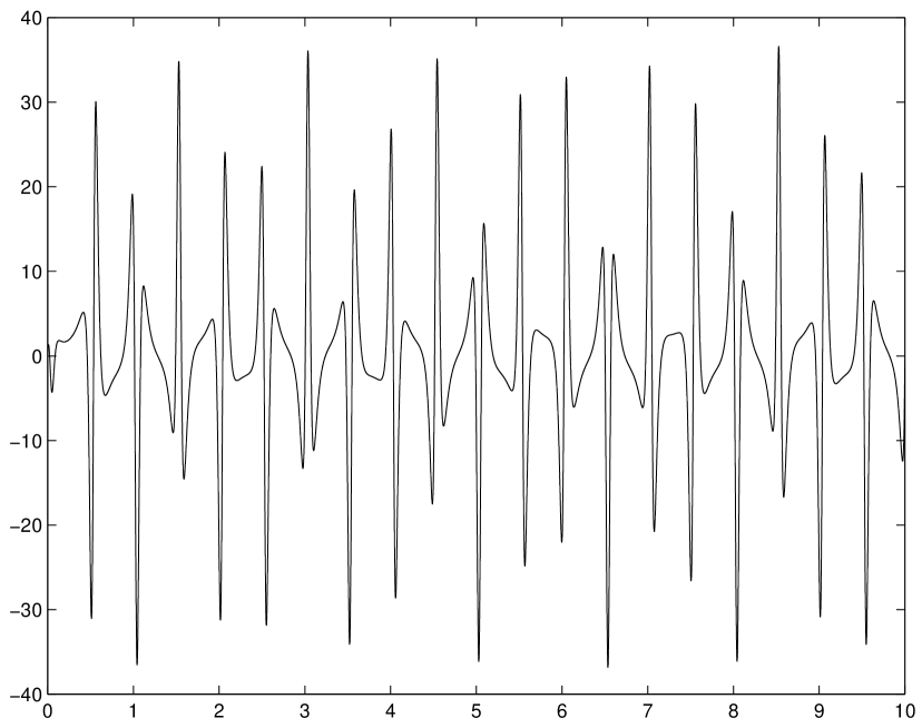
FIG. 1.: $u_{1}$ versus $\tau$ at $x=0$. An overall exponential decay has been compensated for. The scale on the vertical axis is irrelevant, as the equations are linear. On the horizontal axis we have marked background periods, that is $\tau/\Delta$. The sharp peaks are typical features. Although it is not clear from this plot, they are perfectly smooth.

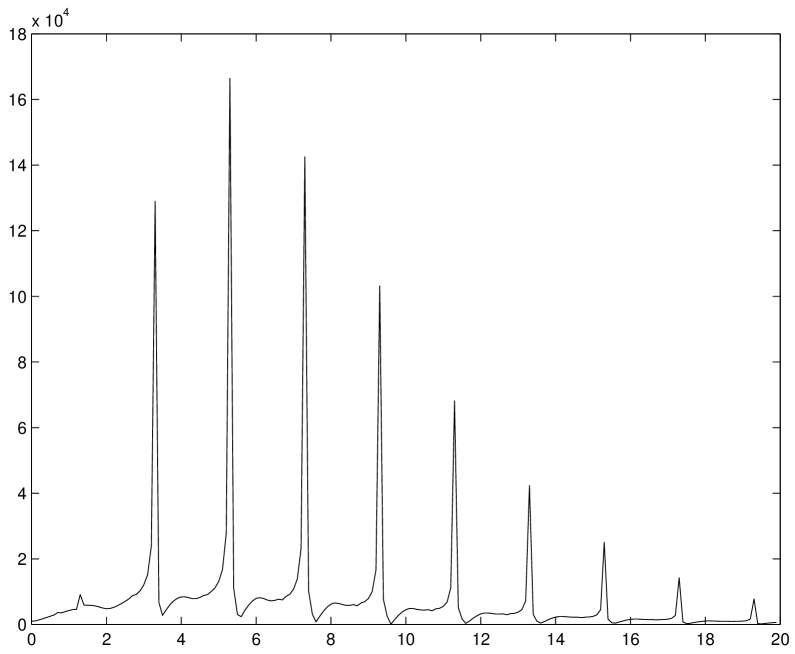
FIG. 2.: The low-frequency end of the discrete Fourier transform of the previous figure. The vertical scale is again irrelevant. On the horizontal axis we have marked frequency in units of the background frequency, that is $(\omega\Delta)/(2\pi)$. The quasiperiodic nature of the signal shows up in the peaks situated at $(\omega\Delta)/(2\pi)=1.3,3.3,5.3,\dots$. The spectrum decays rapidly at high frequencies.

With increasing $l$, the even parity numerical code appears to be more and more sensitive to small errors in the background solution, as the solutions obtained at different resolutions drift apart more and more rapidly. The solution at late times depends sensitively on the initial data, so that the system looks chaotic. This problem may be unavoidable with any code. Our results still seem to capture the correct overall behavior, as the values of $\kappa$ and $\omega$ obtained at different resolutions differ much less than the actual time series. We believe that the explanation is that different resolutions agree reasonably well on the periodic functions $f_{1}$ and $f_{2}$, but that the initial data-dependent coefficients $C_{1}$ and $C_{2}$ take essentially random values at late times for different resolutions.

In summary, we find that both even and odd perturbations decay exponentially for all physical values of $l$. It is clear that perturbations with large $l$ will decay more and more quickly because of the presence of the terms $u_{,\tau}=-lu+\dots$ in all evolution equations. (These terms are introduced by the scaling of perturbations with $r^{l}$ to keep them regular at $r=0$.) The numerical evolutions confirm that higher $l$ modes decay more and more rapidly. We can therefore affirm that all values of $l$ decay, even though we have checked this explicitly only for the lowest few values. The most slowly decaying mode occurs in the $l=2$ polar perturbations, with $\lambda\simeq-0.07\times(1/\Delta)+0.3\times(2\pi i/\Delta)\simeq-0.02+0.55i$. As this mode decays so very slowly, there may be an intermediate range of $p-p_{*}$ for a given one-parameter family of initial data where this perturbation becomes universally visible. For $p-p_{*}$ small enough, however, the spherical universal solution will again dominate.

System			$\left(\kappa\Delta,{\omega\Delta/2\pi}\right)$
grid points	$100$	$200$	$400$	$800$	$1600$
even $l=0$	$9.24,0.0$	$9.21,0.0$	$9.21,0.0$	$9.21,0.0$	$9.21,0.0$
even $l=1$	$-0.34,0.0$	$-0.31,0.0$	$-0.48,0.0$	$noisy$	$-0.30,0.0$
even $l=2$	$-0.08,0.3$	$-0.07,0.3$	$-0.06,0.3$	$-0.07,0.3$	$-0.070.3$
even $l=3$	$-1.63,1.6$	$-1.65,1.6$	$-1.65,1.6$	$-1.65,1.6$	$-1.66,1.6$
even $l=4$	$-2.8,0.9$	$-2.9,0.9$	$-2.9,0.9$	$-3.0,0.9$	$noisy$
even $l=5$	$-4.0,0.2$	$-4.25,0.2$	$-3.9,0.2$	$-3.65,0.3$	$noisy$
odd $l=2$	$-2.20,1.9$	$-2.28,1.9$	$-2.30,1.9$	$-2.30,1.9$	$-1.8,3.0$
odd $l=3$	$-3.13,1.3$	$-3.23,1.4$	$-3.27,1.4$	$-3.28,1.4$	$noisy$
odd $l=4$	$-4.05,0.7$	$-4.20,0.7$	$-4.25,0.7$	$-4.27,0.7$	$noisy$
odd $l=5$	$-5.0,0.0$	$-5.2,0.0$	$-5.2,0.1$	$-5.3,0.1$	$-5.3,0.1$

TABLE I.: Summary of eigenvalues $\lambda$, read off from $u_{1}(x=0,\tau)$. The values of kappa were obtained by eliminating an exponential factor. The values of $\omega$ were obtained from a discrete Fourier transform of the result. Values of $\omega\Delta/2\pi$ are defined modulo $2$, while peaks in the discrete Fourier transform of $u_{1}$ are located at $\omega\Delta/2\pi+1+2N$ for non-negative integer $N$. As we have integrated over a range of $10\Delta$ in $\tau$, $\omega\Delta/2\pi$ can only be estimated in multiples of $0.1$. Results marked “noisy” are dominated by numerical error. In the Fourier transform this shows up as high frequency noise.

System			$\left(\kappa\Delta,{\omega\Delta/2\pi}\right)$
grid points	$100$	$200$	$400$	$800$	$1600$
even $l=2$	$1.1,0.3$	$0.15,0.3$	$0.0,0.3$	$-0.05,0.3$	$-0.07,0.3$
even $l=3$	$0.25,1.4$	$-1.3,1.6$	$-1.55,1.6$	$-1.63,1.6$	$-1.65,1.6$
even $l=4$	$-0.53,0.5$	$-2.0,0.8$	$-2.75,0.9$	$-2.8,1.0$	$noisy$
even $l=5$	$-1.45,1.5$	$-2.77,0.0$	$-3.3,0.1$	$-3.2,0.2$	$noisy$
odd $l=2$	$-1.74,1.8$	$-2.18,1.9$	$-2.30,1.9$	$-2.30,1.9$	$noisy$
odd $l=3$	$-1.95,1.2$	$-2.95,1.3$	$-3.2,1.4$	$-3.25,1.4$	$noisy$
odd $l=4$	$-2.2,0.4$	$-3.55,0.7$	$-4.1,0.7$	$-4.25,0.7$	$noisy$
odd $l=5$	$-2.7,1.4$	$-4.1,1.9$	$-5.0,0.0$	$-5.2,0.1$	$noisy$

TABLE II.: The same with an alternative finite differencing method for $l\geq 2$, defined by Eq. (B10). Note that convergence is much slower, but that for 800 grid points these results agree quite well with those of the other method.

A Background solution

Following Choptuik, we introduce the scale-invariant and dimensionless auxiliary fields for the spherically symmetric scalar field system as

$$X=\sqrt{2\pi}r\varphi^{\prime},\qquad Y=\sqrt{2\pi}r\dot{\varphi},$$ (A1)

in the radial basis. (Do not confuse Y with a spherical harmonic.) We use the dependent variables $g=a/\alpha$, $a$, $X$ and $Y$, and the coordinates $x$ and $\tau$. With the shorthand

$$D\equiv xge^{\xi_{0}}(1-\xi_{0,\tau}),$$ (A2)

the wave equation for $\varphi$ is equivalent to the first-order system

$$x\left(\matrix{X_{,x}\cr Y_{,x}}\right)=\frac{1}{1-D^{2}}\left(\matrix{1&D\cr D&1}\right)\left(\matrix{-[\frac{1}{2}(1+a^{2})+a^{2}(X^{2}-Y^{2})]X+gxe^{\xi_{0}}Y_{,\tau}\cr\ \ \;[\frac{1}{2}(3-a^{2})+a^{2}(X^{2}-Y^{2})]Y+gxe^{\xi_{0}}X_{,\tau}}\right).$$ (A3)

The Einstein equations are

$$xg_{,x} = g(1-a^{2}),$$ (A4)

$$xa_{,x} = \frac{a}{2}[1-a^{2}+2a^{2}(X^{2}+Y^{2})],$$ (A5)

$$a_{,\tau} = -(1-\xi_{0,\tau})xa_{,x}+\frac{2a^{3}}{gxe^{\xi_{0}}}XY.$$ (A6)

In order to exclude a conical singularity at $r=0$, we impose $a=1$ at $x=0$. In order to fix the remaining coordinate ambiguity $t\to f(t)$ we impose $g=1$ at $x=0$. We make $x=1$ an ingoing null surface by imposing $D=1$ at $x=1$. $\xi_{0}$ is not initially known, but is determined together with the dynamical fields $X$, $Y$, $a$ and $g$ of the critical solution.

We have recalculated the background using the numerical code of Gundlach[10], slightly modified to use $x$ instead of $\zeta=\ln x$, which results in a better treatment of $x=0$. If the solution is regular, $X$ and $Y$ vanish at $x=0$. Therefore we work with $X_{2}\equiv x^{-2}X$ and $Y_{1}\equiv x^{-1}Y$. $x=0$ and $x=1$ are regular singular points of the equations. The regularity condition (vanishing of the numerator in the wave equation) is

$$X_{2}={1\over 3}e^{\xi_{0}}\left[Y_{1,\tau}+(1-d\xi_{0}/d\tau)Y_{1}\right]$$ (A7)

at $x=0$, while at $x=1$ it is

$$\left[1+a^{2}(1+2X_{2}^{2}-2Y_{1}^{2})\right]X_{2}+\left[-3+a^{2}(1-2X_{2}^{2}+2Y_{1}^{2})\right]Y_{1}-2\left(1-{d\xi_{0}\over dx}\right)^{-1}\left({\partial Y_{1}\over\partial\tau}+{\partial X_{2}\over\partial\tau}\right)=0.$$ (A8)

The discrete self-similarity of the background is equivalent to periodicity of $X$, $Y$, $a$ and $g$ in $\tau$, with a period $\Delta$ that is initially unknown. $a$ is treated as a functional of $X$, $Y$, $g$ and $\xi_{0}$, by solving equation (A6), with periodic boundary conditions in $\tau$ for each value of $x$. Note that this equation is linear in $a^{-2}$. Periodicity is imposed by representing $X$, $Y$, $g$ and $\xi_{0}$ through a (truncated) Fourier series. $\tau$-derivatives are calculated, and equation (A6) is solved, in Fourier space. This makes the numerical method a pseudo-spectral one. The $y$-derivatives are implemented through finite differencing on a grid equally spaced in $x$, and are solved by relaxation, together with the algebraic and ODE (pseudo-algebraic) boundary conditions at $x=0$ and $x=1$.

We have calculated the background solution using points 51, 101, …, 1601 on the range $0\leq x\leq 1$, always with 128 points per period $0\leq\tau<\Delta$. It was shown in [10] that this resolution in $\tau$ is large enough so that numerical error is dominated by resolution in $x$ and systematic error effects at $x=0$ and $x=1$.

We observe second-order convergence, measured by the maximal and root-mean-squared differences of $X_{2}$, $Y_{1}$, $a$ and $g$, from 51 to 1601 grid points in $x$ (with 128 Fourier components in $\tau$). $\Delta$ and $\xi_{0}$ (in the maximum and root-mean-squared norms) also show convergence, but not to a distinct order. This is illustrated in Fig. 3. For the perturbation calculations we have always used the high-resolution background, downsampled as necessary.

FIG. 3.: Convergence of the background solution with increasing resolution in $x$. On the horizontal axis we plot the logarithm of the number of grid points, on the vertical axis the logarithm of the difference between one numerical solution and the one with half the resolution. The two thick lines are the maximal and root-mean-squared differences (over both $0\leq x\leq 1$ and one period in $\tau$) of all fields. The thin lines are the differences of the “eigenvalue” $\xi_{0}(\tau)$. The dashed line is the difference in the eigenvalue $\Delta$.

B Perturbations numerical method

The perturbation equations are of the form

$${\partial u\over\partial\tau}+A{\partial u\over\partial x}+Bu=0,$$ (B1)

where $u$ is a vector of unknowns, and $A$ and $B$ are background-dependent matrices.

As by definition $x=1$ is an ingoing spherical null surface, the domain of dependence of perturbation data at $\tau=0$, $0\leq x\leq 1$ for $\tau\geq 0$ is precisely $0\leq x\leq 1$. Both scalar and gravitational waves travel only from smaller to larger $x$ for $x\geq 1$. In order to implement a time evolution without an artificial boundary condition at $x=1$, we use an evolution scheme that explicitly uses the characteristic speeds and therefore changes over smoothly to upwind $x$-derivatives for $x\geq 1$. The numerical method we have used is similar to that used for the perturbations of the perfect fluid critical solutions in a previous publication [6, 13], but is second order in space and time. It uses second order one-sided derivatives in $x$, and is Runge-Kutta-like in $\tau$:

$$u^{n+{1\over 2}}_{j} = u^{n}_{j}-{\Delta\tau\over 2}\left[(A_{-})^{n}_{j}{4u^{n}_{j+1}-u^{n}_{j+2}-3u^{n}_{j}\over 2\Delta x}-(A_{+})^{n}_{j}{4u^{n}_{j-1}-u^{n}_{j-2}-3u^{n}_{j}\over 2\Delta x}+B^{n}_{j}u^{n}_{j}\right],$$ (B2)

$$u^{n+1}_{j} = u^{n}_{j}-\Delta\tau\left[(A_{-})^{n+{1\over 2}}_{j}{4u^{n+{1\over 2}}_{j+1}-u^{n+{1\over 2}}_{j+2}-3u^{n+{1\over 2}}_{j}\over 2\Delta x}-(A_{+})^{n+{1\over 2}}_{j}{4u^{n+{1\over 2}}_{j-1}-u^{n+{1\over 2}}_{j-2}-3u^{n+{1\over 2}}_{j}\over 2\Delta x}+B^{n+{1\over 2}}_{j}u^{n+{1\over 2}}_{j}\right].$$ (B3)

Here $A_{+}+A_{-}=A$. In order to use the characteristic speeds in the finite differencing scheme, it is necessary to split $A$ into a sum over its eigenvalues according to their sign, so that, for example,

$$A_{3+}=\lambda_{+}\left(\matrix{{1/2}&-{1/2}&\cr-{1/2}&{1/2}&\cr&&0\cr}\right)+\lambda_{0}\left(\matrix{0&&\cr&0&\cr&&1\cr}\right),\qquad A_{3-}=\lambda_{-}\left(\matrix{{1/2}&{1/2}&\cr{1/2}&{1/2}&\cr&&0\cr}\right)$$ (B4)

For $x\geq 1$, $\lambda_{-}$ becomes positive, so that$A_{+}=A$ and $A_{-}=0$, so that we do not need the downwind derivative there. We go just one grid point beyond $x=1$, so that the last grid point just before $x=1$ still has two points to its right in order to take a right derivative there. All grid points further to the right only require left derivatives. This means that we could have extended the numerical domain to large $x$. We have chosen $0\leq x\leq 1+\Delta x$ because it is the smallest numerical domain in which we stay in the domain of dependence of the perturbation initial data for all $\tau$, while using a one-sided three-point stencil. (If we used a first-order differencing scheme, with two-point stencils, the numerical domain $0\leq x\leq 1$ would be sufficient.)

We might refer to the method just described as the second-order characteristic method. It is explicit and second order. One obtains an implicit method by averaging $u^{n}$ and $u^{n+1}$ to obtain a new improved estimate for $u^{n+1/2}$,

$$u^{n+1/2}=(u^{n}+u^{n+1})/2,$$ (B5)

and iterating the pair (B5,B3) of equations until $u^{n+1}$ has converged. Let us call this the iterated characteristic method.

The boundary $x=0$ does not require special treatment, as $u(-x)=\pm u(x)$ for all $u$, so that ghost grid points with $x<0$ are available for taking derivatives. The one-sided differencing operators do not give exactly zero at $x=0$ even if analytically $\partial u/\partial x(0)=0$, but that is consistent: all terms in the finite difference equations combine so that $u(0)$ remains zero to machine precision if $u$ is odd initially. This also ensures that source terms of the form $u/x$ for odd $u$ in the evolution equations are well behaved numerically.

Another promising candidate for numerical treatment of the equations is the iterated Crank-Nicholson method. In this method, we need to treat the boundaries specially. At $x=0$ we have tried updating the boundary point by extrapolation from its next neighbors at each iteration, taking into account that $u$ is either odd in $x$ (and vanishes at $x=0$) or even in $x$. Alternatively we have used the exact value $\partial u/\partial x=0$ for even $u$ and the finite difference stencil $\partial u/\partial x=[u(\Delta x)-u(0)]/\Delta x$, which is second order at $x=0$ for odd $u$. At $x=1+\Delta x$, we have either used extrapolation, or the one-sided (left side only) second-order stencil of the characteristic methods.

The constraints are solved by integrating from $x=0$ out to $x=1$. For stability, we do not evolve any variable for which we have a constraint, but instead calculate it from the constraints, including at the half-step $n+{1\over 2}$. For simple integrations $du/dx=c$ with $u$ an even function of $x$, and $u(0)$ given, we use the trapezoidal rule

$$u_{j+1}=u_{j}+{\Delta x\over 2}\left(c_{j}+c_{j+1}\right).$$ (B6)

For the ODE $du/dx+bu/x=c$, with $b$ and $c$ even in $x$ and, therefore, $u$ odd in $x$, we use

$$u_{j+1}=u_{j}+\left(1+{\Delta x\,b_{j+1}\over x_{j}+x_{j+1}}\right)^{-1}\left[\left(1-{\Delta x\,b_{j}\over x_{j}+x_{j+1}}\right)+{\Delta x\over 2}(c_{j}+c_{j+1})\right].$$ (B7)

This scheme is second-order accurate at all grid points. For those variables $u$ that are even in $x$ and of $O(1)$ at $x=0$, because $c$ is odd and of $O(x^{-1})$, we use the same scheme, with coefficients $b-1$ and $cx$, in order to first calculate the odd function $\bar{u}=ux$. Then we divide by $x$ to obtain $u$. In this case we extrapolate twice: first $cx$ to $x=0$, and then $\bar{u}/x=u$ to $x=0$.

The perturbations were calculated at different resolutions, related by grid refinements by a factor two in both $x$ and $\tau$. As our lowest resolution, we used $\Delta x=0.01$, with a Courant factor of $\Delta\tau/\Delta x\simeq 0.05$. (The exact Courant factor is chosen so that the number of time steps for integrating the perturbations is a multiple of the number of time steps in the background, per period.) This small Courant factor is necessary for stability, apparently because some coefficients of the perturbation equations, although smooth, have very large gradients in $\tau$ near $x=0$. We have also verified that the effect of using an even smaller Courant factor is negligible. Our highest resolution was finer by a factor of $16$ in both space and time. The background coefficients $a$, $\alpha$, $X$, $Y$ were given in Fourier coefficients at 128 points per period in $\tau$ and the required intermediate values of $\tau$ were obtained by local cubic interpolation. We chose local cubic interpolation as it is much faster than Fourier interpolation, and because of limited computer memory. The interpolation is formally second order accurate, and all background coefficients are well resolved at this resolution. To separate the convergence of the perturbations from that of the background coefficients, we used a background solution obtained with 1601 points in $x$, and downsampled it by factors of 1, 2, 4, 8 and 16.

As a test, we used all numerical methods on the trivial background of flat empty spacetime without a scalar field. On this background, the even matter and metric perturbations decouple. In fact, the even matter perturbation equation is identical to the odd master equation, and both are identical to the free wave equation. We are therefore testing the code on the free wave equation, with angular dependence $Y_{lm}$, and in self-similarity coordinates, on the domain of dependence $0\leq x<1$.

Already in this simple test, we find that the iterated Crank-Nicholson method with any of the boundary treatments discussed is unstable. The instability does not have a continuum limit in space. In fact, it changes sign about every grid point in space, and grows twice as fast in time when $\Delta x$ is halved. Nevertheless, it appears to have a continuum limit in time. The instability changes smoothly from one time step to the next, and in fact, it is practically unchanged if $\Delta\tau$ is reduced by a factor of 10 (at constant $\Delta x$). The instability is most apparent at $x=0$, but in an implicit scheme, all grid points in space are of course linked.

As we have not found a boundary treatment in which iterated Crank-Nicholson is stable, we now restrict ourselves to the two characteristic schemes. In flat space we find that they give essentially the same solution. Both are stable and second-order convergent for a long time. In particular, $x=0$ and $x=1$ are perfectly normal points, as expected from the construction of the numerical scheme. At high resolutions, high $l$, and late times (for example, $\Delta x=1/1600$, $l=6$, $\tau\gtrsim 1$) we see an oscillating instability in $\tau$ near $x=0$ that leads to a breakdown of convergence near $x=0$, and which blows up for sufficiently large $l$ and high resolution. This instability appears to be a solution of the continuum equations, but for initial data which are provided by finite differencing error at late times. To demonstrate this, we have evolved a narrow Gaussian pulse originally centered around $x=0.5$ in flat spacetime. After this pulse has left the computational domain, nothing should happen physically, and we are left with pure numerical error. We then extracted new Cauchy data at a late time, at a high resolution, and restarted these data with different resolutions (in space and time), down-sampling the error data as necessary. For some time we clearly see quadratic convergence, until new numerical error takes over.

The instability is present already in the free wave equation in flat space, which in our rescaled variables and self-similarity coordinates is

$${\partial u_{1}\over\partial\tau}+x{\partial u_{1}\over\partial x}-{\partial u_{2}\over\partial x}-{2l+2\over x}u_{2}-(l+1)u_{1}=0,$$ (B8)

$${\partial u_{2}\over\partial\tau}+x{\partial u_{2}\over\partial x}-{\partial u_{1}\over\partial x}-(l+1)u_{2}=0.$$ (B9)

Recall that for any $l$, $u_{1}$ is an even function of $O(1)$ of $x$ and $u_{2}$ is an odd function of $O(x)$. As the instability is centered at $x=0$ and becomes worse with increasing $l$, it must be linked to the term $u_{2}/x$. We have generalized a well known trick for the spherical wave equation which consists in absorbing this term into the $x$-derivative. We rewrite the equations as

$${\partial u_{1}\over\partial\tau}+x{\partial u_{1}\over\partial x}-(2l+3){\partial(x^{2l+2}u_{2})\over\partial(x^{2l+3})}-(l+1)u_{1}=0,$$ (B10)

$${\partial u_{2}\over\partial\tau}+x(2l+3){\partial(x^{2l+2}u_{2})\over\partial(x^{2l+3})}-{\partial u_{1}\over\partial x}+(l+1)u_{2}=0.$$ (B11)

We then finite difference $u_{2}$ always in the way suggested by the equations, using left and right second-order one-sided derivatives to obtain the characteristic method outlined above. Note that we only ever use the new derivative of $u_{2}$, never the straight derivative $\partial u_{2}/\partial x$. The generalization to the even and odd parity perturbations of scalar field collapse, applied to the variables $u_{2}$ and $u_{5}$, is straightforward. In particular, the coefficients of $\partial u_{2}/\partial x$ and $(2l+2)u_{2}/x$, although now different from unity, remain equal to each other. All other variables $u$ are differentiated directly with respect to $x$. When we use this finite differencing method for the flat space wave equation, the late-time solution that is pure numerical error is now smooth and decays exponentially instead of blowing up, as we had hoped. On the Choptuik background, however, the instability at the center is still not suppressed. Before the instability takes over, the two methods clearly converge towards each other.

We have also tested convergence of the code on the (numerically generated) Choptuik background. Here, stability requires a smaller Courant factor. The differences between different resolutions are peaked at $x=0$ and are smooth functions of $x$. For most values of $\tau$ and $x$ convergence is clearly second order, with the exception of certain value of $\tau$ near $x=0$, where the background coefficients are particularly rapidly varying. Here convergence still occurs (differences between resolutions decrease with resolution), but is not of a clear order: lower than second order for low resolutions and higher than second order for high resolutions. Somewhat surprisingly, second-order convergence disappears and then reappears many times. Apparently error is not just growing with time, but depends very strongly on the background. The explicit and iterated characteristic methods give very similar results. At typical resolutions the differences between the two methods at the same resolution are much smaller than between resolutions. The only exception from this behavior is at early times, when the iterated method clearly shows first-order convergence that goes over smoothly into the expected second-order convergence.

In the flat empty background, pulses with support well inside $x=1$ quickly leave the computational domain. On the Choptuik background, we expect to find (exponentially damped) quasiperiodic behavior at late times. We must therefore evolve to large values of $\tau$ (of the order of 10 to 20 background periods $\Delta$). Not surprisingly we find that second-order convergence breaks down after a period or so, both because the quasiperiodic oscillations at different resolutions drift out of phase, and because the exponential decay rates are slightly different. At early times, we still observe second-order convergence, as described above.

REFERENCES

- [1] M. W. Choptuik, Phys. Rev. Lett. 70, 9 (1993).
- [2] C. Gundlach, Adv. Theor. Math. Phys. 2, 1 (1998), gr-qc/9712084.
- [3] C. R. Evans and J. S. Coleman, Phys. Rev. Lett. 72, 1782 (1994).
- [4] C. Gundlach and J. M. Martín-García, Phys. Rev. D 54, 7353 (1996).
- [5] S. Hod and T. Piran, Phys. Rev. D 55, 3485 (1997).
- [6] C. Gundlach, Phys. Rev. D 57, 7075 (1998)
- [7] A. M. Abrahams and C. R. Evans, Phys. Rev. Lett. 70, 2980 (1993)
- [8] U. H. Gerlach and U. K. Sengupta, Phys. Rev. D 19, 2268 (1979).
- [9] U. H. Gerlach and U. K. Sengupta, Phys. Rev. D 22, 1300 (1980).
- [10] C. Gundlach, Phys. Rev. Lett. 75, 3214 (1995); Phys. Rev. D 55, 695 (1997).
- [11] F. J. Zerilli, J. Math. Phys. 11, 2203 (1970)
- [12] T. Regge and J. A. Wheeler, Phys. Rev. 108, 1063 (1957).
- [13] R. J. LeVeque, Numerical methods for conservation laws, Birkhäuser, Basel 1992.