Exact relativistic stellar models with liquid surface.
I. Generalizing Buchdahl’s $n=1$ polytrope.

Abstract

A family of exact relativistic stellar models is described. The family generalizes Buchdahl’s $n=1$ polytropic solution. The matter content is a perfect fluid and, excluding Buchdahl’s original model, it behaves as a liquid at low pressures in the sense that the energy density is non-zero in the zero pressure limit. The equation of state has two free parameters, a scaling and a stiffness parameter. Depending on the value of the stiffness parameter the fluid behaviour can be divided in four different types. Physical quantities such as masses, radii and surface redshifts as well as density and pressure profiles are calculated and displayed graphically. Leaving the details to a later publication, it is noted that one of the equation of state types can quite accurately approximate the equation of state of real cold matter in the outer regions of neutron stars. Finally, it is observed that the given equation of state does not admit models with a conical singularity at the center.

1 Introduction

Among the new exact relativistic stellar models recently found in [1, 2], two families are of particular physical interest. They both generalize gaseous models found by Buchdahl [3, 4]. His models have equations of state which reduce to a Newtonian polytropic gas (of index $n=1$ and $n=5$ respectively) at low pressures. We will refer to the generalized solutions as the generalized Buchdahl $n=1$ polytrope (GB1) and generalized Buchdahl $n=5$ polytrope (GB5) models respectively. By contrast to Buchdal’s original solutions the generalized models have equations of state which are liquid at low pressures in the sense that the density is non-zero at zero pressure, $\rho_{\rm s}>0$. Their equations of state each have two free parameters. By properly adjusting those parameters, the models can describe the interior of neutron stars with surprising accuracy. In this paper we describe the GB1 family [1]. The matter in the model is a perfect fluid obeying a certain barotropic equation of state $p=p(\rho)$. The history of static spherically symmetric (SSS) models with matter goes back to Schwarzschild’s discovery already in 1916 of his interior solution with incompressible matter [5]. Although a number of exact SSS models have been found since then (see e.g. Tolman’s classic paper [6]) there is an important distinction which should be made between solutions such as Schwarzschild’s interior solution and solutions of Tolman’s type. Whereas the former kind is a family of solutions describing a stellar sequence with varying masses for the given equation of state ($\rho=constant$ in that case) the latter kind gives only a single solution with a fixed mass once the equation of state is specified. The underlying reason is that Schwarzschild’s interior model is the general solution of the Einstein field equations for the given equation of state. By general solution we mean a solution with the full number of integration constants. For any given equation of state there is a family of SSS models parametrized by precisely two physically relevant integration constants. Usually one of these constants is determined by requiring that the stellar model is regular at the center. The single remaining nontrivial integration constant then determines the total mass.

The general solutions correspond to nontrivial symmetries of the field equations. Such symmetries only exist for certain special equations of state [1]. Tolman type solutions on the other hand are particular solutions which do not contain the full number of integration constants. Such special solutions have been referred to as submanifold solutions since they correspond to submanifolds in the phase space which are left invariant by the field equations [7]. Obviously the general solutions are more useful than the submanifold solutions. However, until recently Schwarzschild’s interior solution was the only general SSS solution which was considered to be of physical interest.

At this point we should make clear what we mean by a physically interesting solution. For the purposes of this paper we consider a solution to be physical if the energy density is non-negative, $\rho\geq 0$ (gravity is attractive), and that the matter is locally mechanically stable so that $p\geq 0$ and $dp/d\rho\geq 0$. Incompressible matter is considered to be included in this category. Schwarzschild’s interior solution was the first matter filled general physical SSS solution of the Einstein equations. It took almost half a century before the next general physical SSS model, the $n=5$ polytrope solution, was discovered by Buchdahl in 1964 [4]. As in the case of a Newtonian $n=5$ polytrope this solution has an infinite radius although the mass is finite. This model was not considered to be of any significant physical interest. A few years later Buchdahl found the $n=1$ polytrope solution [3]. Although this model has a finite radius it has not been widely discussed in the literature. The next development came recently when the generalizations of Buchdahl’s solutions were discovered by Simon [2] and Rosquist [1]. The GB1 and GB5 solutions are in fact families of solutions with equations of state depending on two continuous parameters. In the present paper we discuss the GB1 family in some detail. Because of the two parameters the structure of this family is quite rich with qualitative behaviour varying in different parts of parameter space. In particular, by an appropriate choice of the equation of state parameters, the GB1 family can be fitted quite accurately to the Harrison-Wheeler (HW) equation of state [8] for cold matter expected to be valid in the outer parts of a neutron star. Later refinements of the HW equation of state are essentially corrections in the regime above nuclear densities. The fitting will be performed in a separate paper [9]. It turns out that the best fit GB1 model is very close to the original Buchdahl solution rendering that model more interesting than previously thought. As for the GB5 family, its basic properties are planned to be discussed in a forthcoming paper [10] (see also [11]).

One reason that the new static models are interesting is that they can serve as starting points to find an interior solution for the Kerr metric. Assuming that such an interior general physical solution exists, and that it is valid for a slowly rotating Kerr exterior, there must be an SSS interior solution in the limit of zero rotation. Furthermore, this static limit will also be a general physical solution because of the arbitrary mass parameter which is present in the Kerr metric. Of course this heuristic argument excludes interiors with singular matter distributions such as the Negebauer-Meinel disk [12]. Referring to the extensive classification of general SSS models in [1], the GB1 and GB5 solutions are in fact the only good candidates for the static limit of a possible interior Kerr solution. On the other hand it is quite conceivable that there are rotating generalizations of the GB1 and GB5 models (as of any fluid SSS model) which have an exterior vacuum field which is different from Kerr. One might try to spin up the GB1 model to yield a rotating perfect fluid solution which may or may not have an exterior gravitational field which coincides with the Kerr solution. Attempts in this direction have been made by trying to extend the use of the Newman-Janis trick [13] to impart rotation to fluid SSS models [14, 15] but without success so far. However, the GB1 or GB5 models so far have not been considered in this context.

Exact SSS solutions may also serve as benchmarks to test the numerical codes for integrating the equations of stellar structure. Such testing was performed for example in [16] using the exact solution for the $n=1$ Newtonian polytrope. The existence of exact relativistic solutions with physically reasonable equations of state make it possible to test such codes also in the relativistic domain.

Another important use for exact solutions is to investigate in more detail how the maximum mass depends on properties of the equation of state. Only general physical solutions qualify as objects to study in this context since it is necessary to vary the mass while keeping the equation of state fixed. However, in the past there was no exact model available which was capable of exhibiting a mass maximum. The reason is that the mass maximum requires a rather soft equation of state by contrast to the hardest conceivable matter, the incompressible perfect fluid, which makes up the matter source for the interior Schwarzschild solution. The GB1 models which are the subject of this paper also contain matter which is too hard for a mass maximum to appear. However, as will be shown in [10], the GB5 models have a softer equation of state and do exhibit a mass maximum.

In addition to the topics discussed above the GB1 models have also turned out to be interesting from the point of view of understanding the space of solutions of the SSS Einstein equations. Taking the case of an incompressible fluid as an example, one of the two physically relevant integration constants is determined by the requirement that the metric should be regular at the center. This is sometimes referred to as the condition of elementary flatness. The center is defined as that value of the radial parameter for which the area of the 2-sphere of constant radius tends to zero. However, as described in section 3 the GB1 models have a different behaviour in this respect. It turns out that a GB1 model can only be continued to the center for one specific value of one of the integration constants. The condition of elementary flatness is then automatically satisfied. The global behaviour of singular GB1 models therefore seem to be different from that of singular incompressible models. A discussion of possible singularity types for SSS models was given in [17] but we have not made an attempt to see how the GB1 models would fit in that scheme.

2 The model

The usual starting point when studying SSS models is to write down the metric in Schwarzschild coordinates

$$ds^{2}=-{\rm e}^{2\nu}dt^{2}+{\rm e}^{2\lambda}dr^{2}+r^{2}d\Omega^{2}\ ,$$ (1)

where

$$d\Omega^{2}=d\theta^{2}+\sin^{2}\!\theta\,d\phi^{2}\ ,$$ (2)

is the metric of the 2-sphere and $\nu$ and $\lambda$ are functions of Schwarzschild’s radial variable, $r$. However, this form of the metric is not general enough in the sense that it is not possible to express all exact solutions in closed form using Schwarzschild coordinates. It is therefore useful to write the SSS metric in terms of a general radial variable, $R$,

$$ds^{2}=-{\rm e}^{2\nu}dt^{2}+N^{2}dR^{2}+W^{2}d\Omega^{2}\ ,$$ (3)

where $N$ and $W$ are both functions of $R$. Schwarzschild’s radial variable then becomes a derived quantity given by $r=W(R)$. The form of the metric (3) reflects the free gauge choice of the radial variable expressed by the freedom to choose the radial gauge function $N$. To write down the GB1 model we use the gauge $N={\rm e}^{-\nu}$. The SSS metric then becomes

$$ds^{2}=-Zdt^{2}+Z^{-1}dR^{2}+W^{2}d\Omega^{2}\ ,$$ (4)

where $W$ and $Z:={\rm e}^{2\nu}$ are functions of the radial parameter $R$. Since $N>0$, the radial variable $R$ is increasing outwards from the center of the star. The Schwarzschild radial variable is given by $r=W(R)$. The center of the star is therefore located at $R=R_{\rm c}$ defined by the condition $W(R_{\rm c})=0$. The GB1 model is defined by [1]

$$\begin{split}&Z=V/W\ ,\qquad W=T+X\ ,\qquad V=T-X\ ,\\ &T=\begin{cases}(\omega_{-})^{-1}(\cosh\zeta)\sin[\omega_{-}(R-R_{-})]\ ,&\text{for $\delta>1$ \ ,}\\ (\cosh\zeta)(R-R_{-})&\text{for $\delta=1$ \ ,}\end{cases}\\ &X=(\omega_{+})^{-1}(\sinh\zeta)\sin[\omega_{+}(R-R_{+})]\ ,\end{split}$$ (5)

where $\omega_{\pm}=\sqrt{2\kappa a(\delta\pm 1)}$ and $\zeta>0$. The parameters $\zeta$ and $R_{\pm}$ are integration constants while the parameters $a$ and $\delta$ characterize the equation of state. The latter can be parametrized as

$$p=a(Z^{2}-2\delta Z+1)\ ,\qquad\rho=a(-5Z^{2}+6\delta Z-1)\ ,$$ (6)

where $a>0$ and $\delta\geq 1$. As discussed in [1], models with $\delta<1$ also exist but can only be used in the pressure region $p\geq a(1-\delta^{2})$. The range of $\delta$ will be further restricted below. From the physical point of view, $a$ is a scaling parameter. Models with different values of $a$ can be transformed into each other by simply scaling the metric. The parameter $a$ represents an overall scaling of length scales in the model. A model with given $a$ has a natural length scale given by $\ell=(\kappa a)^{-1/2}$. However, scale invariant physical quantities such as surface redshift are unaffected by changes in $a$. As will be explained below the parameter $\delta$ can be interpreted as a measure of the stiffness of the matter. We will refer to it as the stiffness parameter. The integration constants are not all physical. Only $\zeta$ and the difference $D:=R_{+}-R_{-}$ carry physical information. This is because $D$ is invariant under translations of $R$. Because of its nature as a metric coefficient $Z$ must be strictly positive. Physical requirements on the equation of state further restrict the range of $Z$ as discussed in the next section.

Expressing the functions $T$ and $X$ in terms of $r$ and $Z$ we have

$$T=\textstyle{\frac{1}{2}}r(1+Z)\ ,\qquad X=\textstyle{\frac{1}{2}}r(1-Z)\ .$$ (7)

Since the conditions $r\geq 0$ and $Z>0$ must hold in the stellar interior it follows that $T\geq 0$. Also, as shown below in (12), we have that $Z\leq 1$ which shows that $X\geq 0$.

2.1 The equation of state

In this paper we assume that the energy density is non-negative, $\rho\geq 0$, and that the matter is mechanically stable so that $p\geq 0$ and $dp/d\rho\geq 0$. It follows immediately from (6) that the condition $p\geq 0$ is satisfied precisely if

$$Z\leq Z_{\rm s}=\delta-\sqrt{\delta^{2}-1}\ ,$$ (8)

where $Z_{\rm s}$ denotes the value of $Z$ at the star surface defined by the condition $p=0$. Also, the relation

$$\frac{dp}{d\rho}=\frac{\delta-Z}{5Z-3\delta}\ .$$ (9)

together with $Z>0$ implies that the condition $dp/d\rho\geq 0$ is equivalent to the relation

$$\frac{3\delta}{5}<Z\leq\delta\ .$$ (10)

The speed of sound is given by $u:=\sqrt{dp/d\rho}$. It reaches the speed of light, $u=c=1$, at $Z_{*}=2\delta/3$. It is sometimes of interest to allow superluminal sound speeds for example to obtain a simple model such as Schwarzschild’s interior solution. The limit in which the speed of sound becomes superluminal will be referred to as the causal limit and denoted by an asterisk subscript. The pressure at the causal limit is given by $p_{*}=a(1-8\delta^{2}/9)$ and the corresponding energy density is $\rho_{*}=a(16\delta^{2}/9-1)$. At zero pressure the energy density is $\rho_{\rm s}=4a(1-\delta^{2}+\delta\sqrt{\delta^{2}-1})$. The speed of sound at the surface is given by

$$u_{\rm s}^{2}=\frac{\sqrt{\delta^{2}-1}}{2\delta-5\sqrt{\delta^{2}-1}}\ .$$ (11)

It follows from this expression that the zero pressure sound speed reaches the speed of light at $\delta=\delta_{*}:=3\sqrt{2}/4\approx 1.061$ and becomes infinite in the limit $\delta\rightarrow\delta_{\infty}:=5/\sqrt{21}\approx 1.091$. Thus models with $\delta>\delta_{*}$ have a superluminal speed of sound for all physcially allowed values of the pressure while models with $\delta\leq\delta_{*}$ are causal for $p<p_{*}$ and acausal or $p>p_{*}$.

The upper limit in (8) must be strictly larger than the lower limit in (10). This gives the additional restriction $\delta<\delta_{\infty}$ and then

$$\frac{3\delta}{5}<Z\leq\delta-\sqrt{\delta^{2}-1}\leq 1\ .$$ (12)

It can be checked that the condition $\rho\geq 0$ is always satisfied if $\delta\geq 1$ and $Z$ is in the range (12).

An important physical characteristic of the equation of state is the relativistic adiabatic index defined by

$$\gamma=\left(1+\frac{\rho}{p}\right)\frac{dp}{d\rho}\ .$$ (13)

It can be interpreted physically as a compressibility index. Lower $\gamma$-values correspond to softer matter. For the GB1 model the adiabatic index is given by

$$\gamma=\frac{4Z(\delta-Z)^{2}}{(5Z-3\delta)(Z^{2}-2\delta Z+1)}\ .$$ (14)

For models with $\delta>1$ the adiabatic index tends to infinity at the surface while $\gamma_{\rm s}=2$ for Buchdahl’s original model ($\delta=1$). The adiabatic index also tends to infinity in the limit $Z\rightarrow Z_{\infty}:=3\delta/5$ corresponding to $v_{\rm sound}\rightarrow\infty$. At the causal limit the adiabatic index is given by $\gamma_{*}=8\delta^{2}/(9-8\delta^{2})$.

In practical calculations it is convenient to use $\xi:=\omega_{-}/\omega_{+}=\sqrt{(\delta-1)/(\delta+1)}$ as a stiffness parameter in place of $\delta$. The value $\xi=0$ (Buchdahl’s original model) corresponds to the softest equation of state within the GB1 family. The range of $\xi$ is

$$0\leq\xi<\xi_{\infty}:=\frac{1}{2}(5-\sqrt{21})\approx 0.2087\ .$$ (15)

The causal limit is at $\xi=\xi_{*}:=3-2\sqrt{2}\approx 0.1716$. The parameter $\xi$ can be interpreted physically in terms of the speed of sound. Using (6) and (9) and defining $k:=p/\rho$ we find that

$$\xi =\frac{\sqrt{d}}{\sqrt{d_{1}}+\sqrt{d_{2}}}\ ,$$ (16a)

where

$$d :=d_{1}-d_{2}=4u^{2}(u^{2}-2k-5u^{2}k)\ ,$$ (16b)

$$d_{1} :=(k+1)(1+5u^{2})^{2}\ ,$$ (16c)

$$d_{2} :=k+1+2(9k+5)u^{2}+3(15k+7)u^{4}\ .$$ (16d)

In the limit $k\rightarrow 0$ this reduces to

$$\xi=\frac{2u_{\rm s}^{2}}{1+5u_{\rm s}^{2}+\sqrt{1+10u_{\rm s}^{2}+21u_{\rm s}^{4}}}=u_{\rm s}^{2}+\mathcal{O}(u_{\rm s}^{4})\ .$$ (17)

The inverse of this relation takes the simple form $u_{\rm s}^{2}=\xi/\mu$ where we have defined the parameter $\mu:=1-5\xi+\xi^{2}$ which takes values in the interval $0<\mu\leq 1$. Thus for $u_{\rm s}\ll 1$ we see that $\xi$ is essentially the sound speed squared. Assuming that the material in a cold star at low pressure consists of pure iron we can get a rough estimate of the value of $\xi$ for a realistic stellar model. The speed of sound in iron is $6\cdot 10^{5}cm/s$ [18] corresponding to $u=2\cdot 10^{-5}$ in geometrized units. Inserting this value in (16) gives $\xi\sim 4\cdot 10^{-10}$. This value is not sensitive to the value of $p$ for moderate pressures up to and beyond $p=1$ atm. In [9] we will determine $\xi$ more precisely by fitting the GB1 equation of state to the HW equation of state. This will also involve a determination of the scaling parameter $a$.

Figure 1: The two equation of state parameters $x_{0}$ and $x_{1}$ are plotted against $\xi$ using logarithmic scales. Both $x_{0}$ and $x_{1}$ tend to infinity in the limit $\xi\rightarrow\xi_{\infty}\approx 0.2087$. They are both approximately unity at $\xi=0.06$.

It is also convenient to replace $Z$ by a new normalized parameter, $x$, which takes values in the interval [0,1] with $x_{\rm s}=0$ and $x_{\infty}=1$. This is accomplished by the transformation $Z=Kx+Z_{\rm s}$ where $K:=Z_{\infty}-Z_{\rm s}=-(2/5)\mu/(1-\xi^{2})$ and $Z_{\rm s}=(1-\xi)/(1+\xi)$ which implies

$$p =bx(x+x_{0})\ ,$$ (18a)

$$\rho =5b(-x^{2}+2x+x_{1})\ ,$$ (18b)

where $b=aK^{2}$ and

$$x_{0}=10\xi\mu^{-1}\ ,\quad x_{1}=10\xi(1-\xi)^{2}\mu^{-2}\ .$$ (19)

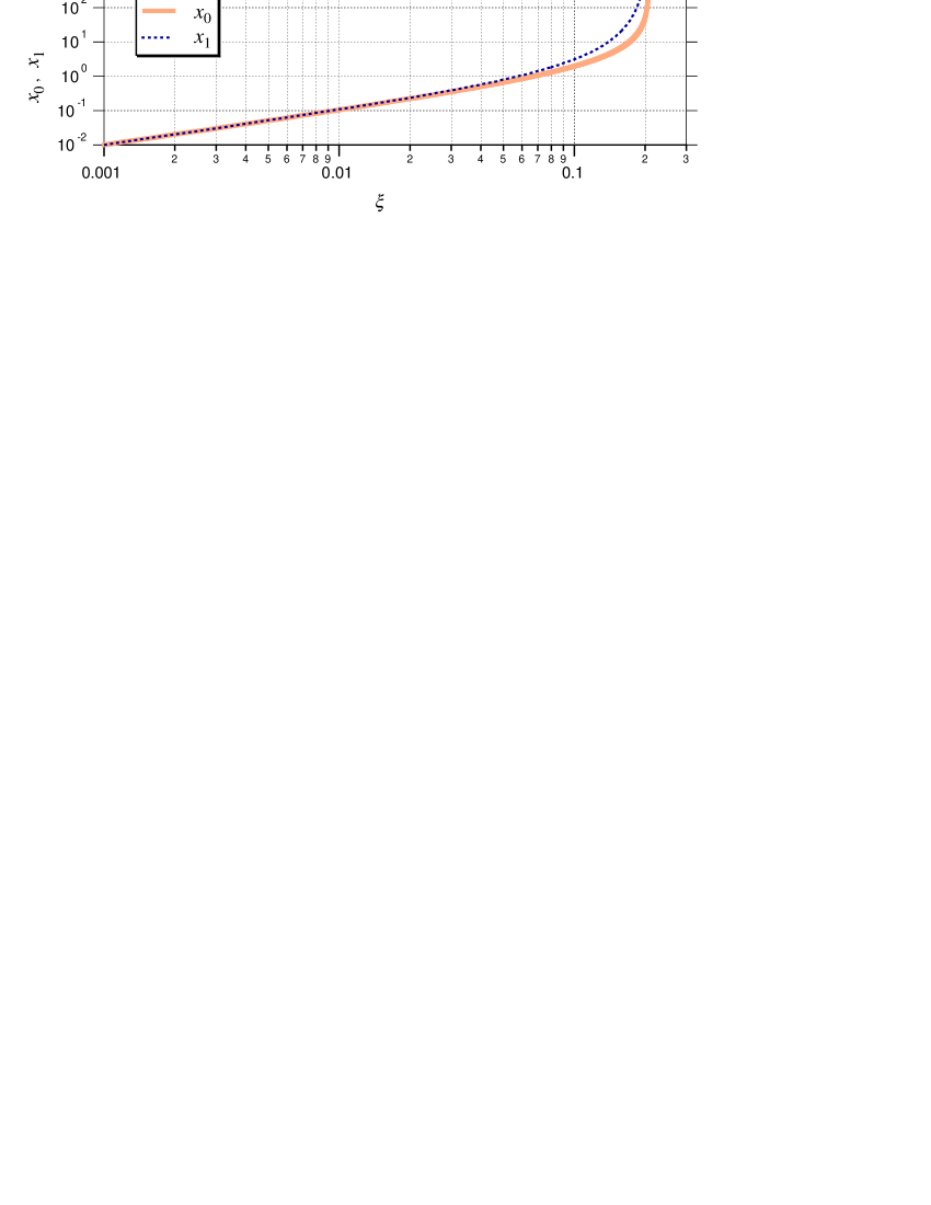
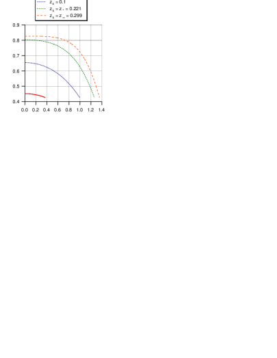
These constants satisfy the inequality $0\leq x_{0}\leq x_{1}$. They are plotted as functions of $\xi$ in figure 1. We see that $x_{0}$ and $x_{1}$ are approximately equal up to $\xi\sim 0.06$ corresponding to $x_{0},x_{1}\lesssim 1$. In the expression for the pressure (18a) the term $x_{0}$ comes into play if $x_{0}\gtrsim x$. Similarly in the expression for the energy density (18b) the term $x_{1}$ is important if $x_{1}\gtrsim x(2-x)$. Since the functions $x$ and $x(2-x)$ both take values in the interval $[0,1]$, this leads to a rough subdivision of the GB1 equations of state into the four types

$$\begin{array}[]{rll}\mbox{(I)}&x_{0}=x_{1}=0&(\xi=0)\ ,\\ \mbox{(II)}&0<x_{0},x_{1}\ll 1&(0<\xi\lesssim 0.001)\ ,\\ \mbox{(III)}&x_{0},x_{1}\sim 1&(0.001\lesssim\xi\lesssim 0.2)\ ,\\ \mbox{(IV)}&x_{0},x_{1}\gg 1&(0.2\lesssim\xi<\xi_{\infty}\approx 0.2087).\end{array}$$ (20)

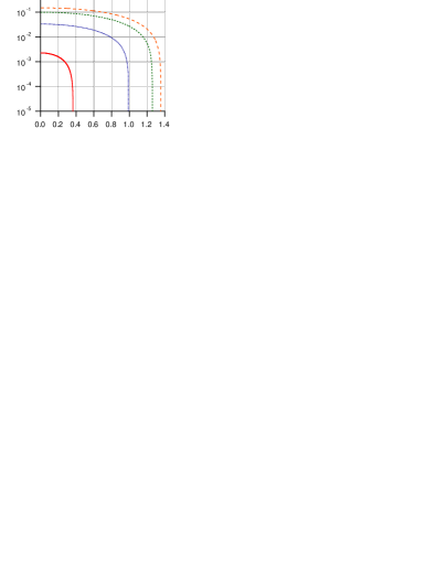
As discussed above, comparison with the actual equation of state of cold matter at low pressure demands $\xi\sim 4\cdot 10^{-10}$ corresponding to a type II equation of state. The four different types of equation of state are plotted in figures 2 and 3. The type I and II equations of state are practically indistinguishable in figure 2 but differ drastically in the behaviour of $\gamma$ in the zero pressure limit as illustrated in figure 3.

\psfrag{prho_left}{\Large$\hat{p},\hat{\rho}$}\psfrag{prho_bottom}{\Large$x$}\includegraphics{prho.eps}

Figure 2: The pressure and the energy density are plotted for four values of $\xi$ representing the different types of equation of state as discussed in the text. For each of these values the upper curve corresponds to the normalized energy density while the lower curve gives the normalized pressure. The causal limit $\rho=\rho_{*}$ in this diagram is the line $\hat{\rho}=1$.

\psfrag{gamma_left}{\Large$\gamma$}\psfrag{gamma_bottom}{\Large$\xi$}\includegraphics{gamma.eps}

Figure 3: The adiabatic index for the $n=1$ Buchdahl equation of state and some of its generalizations. The pressure is scaled by the pressure $p_{\infty}$ at which the adiabatic index becomes infinite. For $\xi>0$ the adiabatic index diverges in the zero pressure limit. The indicated causal limit is the boundary between the regions with subluminal and superluminal sound velocity. It is seen that the causal region defined by subluminal sound speed is located in the lower left hand corner of the diagram with a narrow section stretching towards infinity along the $\gamma$-axis. Models with $\xi<\xi_{*}=3-2\sqrt{2}\approx 0.1716$ start in the causal region at low pressures and enter the acausal region at the pressure $p_{*}$ while the models with $\xi>\xi_{*}$ are acausal for all pressures.

In figure 2 the pressure and energy density are plotted as functions of $x$ and normalized by the energy density at the causal limit which occurs at

$$x=x_{*}:=\frac{5(1-6\xi+\xi^{2})}{6(1-5\xi+\xi^{2})}\ .$$ (21)

The energy density and pressure in that limit are given by

$$\rho_{*}=\textstyle{\frac{25}{36}}b\mu^{-2}(7+\xi^{2})(1+7\xi^{2})\ ,\qquad p_{*}=\textstyle{\frac{25}{36}}b\mu^{-2}(1-34\xi^{2}+\xi^{4})\ .$$ (22)

Since any given value of $\rho$ corresponds dimensionally to a pressure $\rho c^{2}$ it is reasonable to normalize both the energy density and the pressure by $\rho_{*}$. The dimensionless normalized pressure and energy density then become

$$\begin{split}\hat{p}:=p/\rho_{*}&=\hat{b}\,x(x+x_{0})\ ,\\ \hat{\rho}:=\rho/\rho_{*}&=5\hat{b}(-x^{2}+2x+x_{1})\ ,\end{split}$$ (23)

where

$$\hat{b}:=\frac{36(1-5\xi+\xi^{2})^{2}}{25(7+\xi^{2})(1+7\xi^{2})}\ .$$ (24)

To see the full picture when plotting $\gamma$ we use the pressure $p_{\infty}$ at which $\gamma$ tends to infinity as a reference point. Setting $x=1$ in (18a) gives

$$p_{\infty}=b\cdot\frac{1+5\xi+\xi^{2}}{1-5\xi+\xi^{2}}\ .$$ (25)

Then we have

$$p/p_{\infty}=\tilde{b}\,x(x+x_{0})\ ,$$ (26)

where

$$\tilde{b}=\frac{1-5\xi+\xi^{2}}{1+5\xi+\xi^{2}}\ .$$ (27)

Writing the adiabatic index in terms of the normalized parameter gives

$$\gamma=\frac{2(5\xi+\mu x)^{2}[\mu(5-2x)+15\xi]}{5\mu^{2}x(1-x)(10\xi+\mu x)}\ .$$ (28)

For Buchdahl’s polytrope this reduces to

$$\gamma=\frac{2(5-2x)}{5(1-x)}\ .$$ (29)

At zero pressure we have $\gamma=2$ for this model. For the models with $\xi>0$ the adiabatic index instead tends to infinity in that limit with the asymptotic form $\gamma\approx\rho_{\rm s}u_{\rm s}^{2}p^{-1}$.

3 Physical characteristics of the stellar model

In this section we compute some of the general physical characteristics of the GB1 family. As already stated the actual fitting to the HW equation of state will be done in the sequel paper [9]. First we briefly discuss criteria which determine the degree to which the star may considered as relativistic. One such criterion is the surface redshift $z_{\rm s}$ which in principle can be measured directly. In practice, however, this seems to be unrealistic for neutron stars. However, redshifts can be determined indirectly if the mass and radius of the star is known. The surface redshift is given by the formula $z_{\rm s}=(1-2\beta)^{-1/2}-1$ where $\beta:=M/r_{\rm s}$ (see e.g. [19]). A given value of the redshift corresponds to an equivalent velocity through the Doppler relation $1+z=\sqrt{(1+v/c)/(1-v/c)}$. For a Newtonian star, $z_{\rm s}\ll 1$. Defining a star to be relativistic if the surface redshift corresponds to a velocity greater than one percent of the speed of light this would then be the case if $z\gtrsim 0.01$. In principle the redshift can attain values from the Newtonian $z_{\rm s}=0$ up to Buchdahl’s limit [20] $z_{\rm s}=2$ (corresponding to $r_{\rm s}>\textstyle{\frac{9}{4}}M$) which is the maximum redshift if the density is assumed to be non-increasing in the outward direction, $d\rho/dr\leq 0$. In practice, however, the surface redshift of a neutron star is expected to be in the range $0.1\lesssim z_{\rm s}\lesssim 0.9$ [21]. Another criterion can be formulated by considering the deviation from Euclidean geometry. This deviation can be defined as the quantity $\alpha:=1-r/R_{\rm prop}$ where $R_{\rm prop}$ is the proper radial distance defined for a general SSS metric by $R_{\rm prop}=\int_{R_{\rm c}}N{\rm d}R$. The star can then be said to be relativistic if, say, $\alpha_{\rm s}\gtrsim 0.01$.

Regular stellar models must satisfy the condition for elementary flatness at the center. This can be conveniently expressed in terms of the Schwarzschild radial gauge function which for the GB1 models is given by [1]

$$N_{\rm Schw}=Z^{-1/2}(W_{,R})^{-1}\ .$$ (30)

The elementary flatness condition then takes the form

$$\lim_{r\rightarrow 0}N_{\rm Schw}=1\ .$$ (31)

Using (30) it can be written as $Z_{\rm c}^{1/2}(W_{,R})_{\rm c}=1$. From (5) we find $(X_{,R})_{\rm c}=\cosh\zeta$, $(X_{,R})_{\rm c}=\cosh\zeta$. This implies $(W_{,R})_{\rm c}={\rm e}^{\zeta}$, $(V_{,R})_{\rm c}={\rm e}^{-\zeta}$ and $Z_{\rm c}=(V/W)_{\rm c}=(V_{,R})_{\rm c}/(W_{,R})_{\rm c}={\rm e}^{-2\zeta}$.

In the remainder of this paper we will assume that the GB1 equation of state is valid throughout the star. Since $Z$ is bounded it then follows from (7) that $T$ and $X$ both vanish at the center of the star. Using the translational freedom in $R$ we may set $R_{\rm c}=0$. The condition $T(0)=0$ then implies $R_{-}=0$ for $\xi=0$ and that $\omega_{-}R_{-}$ is a multiple of $\pi$ for $\xi>0$. Moreover, to ensure that $T$ is positive as $R$ increases away from the center $\omega_{-}R_{-}$ must actually be an even multiple of $\pi$. Similarly, the condition $X(0)=0$ implies that $\omega_{+}R_{+}$ must also be an even multiple of $\pi$. As already stated in [1] we may then set $R_{\pm}=0$ without loss of generality.

Let us pause for a moment to digest what is actually implied here. We have the curious situation that the mere assumption that the model can be continued to the center of the star implies the vanishing of one of the essential integration constants ($D=R_{+}-R_{-}=0$). Technically this has happened because the function $W(R)$ which gives Schwarzschild’s radial variable is built up by two non-negative terms, $r=W(R)=T(R)+X(R)$, which must both vanish separately at $R=0$. Normally one would expect to use that integration constant to ensure the elementary flatness of the model at the center. So what about elementary flatness?

It follows that the model in fact satisfies the elementary flatness condition [1]. It seems that the GB1 equation of state cannot support a conical singularity at the center. This result sparks off a number of questions. For example, what equations of state have this property of not allowing conical singularities? Also, since a conical singularity is not allowed, in what way does the model break down if we let say $R_{+}$ be nonzero? The answer to the latter question is that the equation of state itself becomes unphysical in the sense that $u\rightarrow\infty$ at some value of the Schwarzschild radial variable, $r=r_{\infty}>0$. At still smaller radii, $r<r_{\infty}$, the matter becomes mechanically unstable, $dp/d\rho<0$. Thus by allowing a nonzero $R_{+}$ what happens is that the matter becomes unphysical before any breakdown in the geometry as we move towards lower $r$-values.

The radius of the star is defined as $r_{\rm s}=W(R_{\rm s})$. The star mass can be computed by the formula [1]

$$M=\textstyle{\frac{1}{2}}\left[W(1-N_{\rm Schw}^{-2})\right]_{\rm s}\ .$$ (32)

This leads to the following expressions for the physical parameters $M$, $\beta$ and $z_{\rm s}$

$$M=\textstyle{\frac{1}{2}}r_{\rm s}\left[1-Z(W_{,R})^{2}\right]_{\rm s}\ ,\qquad\beta=\textstyle{\frac{1}{2}}\left[1-Z(W_{,R})^{2}\right]_{\rm s}\ ,\qquad 1+z_{\rm s}=Z_{\rm s}^{-1/2}(W_{,R})_{\rm s}^{-1}\ .$$ (33)

To evaluate these expressions at the surface we need to know $R_{\rm s}$. Using (5) and (8) we find that $R_{\rm s}=q/\omega_{+}$ where $q$ is defined to be the smallest positive root of the equation $\sin(\xi x)=\eta\sin x$ where we have defined $\eta:=\tanh\zeta$. Thus $q$ satisfies

$$\sin(\xi q)=\eta\sin q\ .$$ (34)

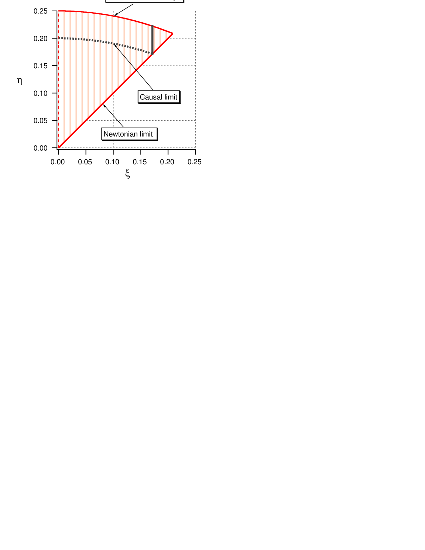
For Buchdahl’s original model ($\xi=0$) we have $q=\pi$ and $R_{\rm s}=\pi/(2\sqrt{\kappa a})$. For $\xi\neq 0$ equation (34) cannot be solved explicitly. Now what about the size of $\eta$ compared to $\xi$? In fact $e^{-2\zeta}=Z_{\rm c}$ is constrained by the requirement $Z_{\infty}<Z_{\rm c}<Z_{\rm s}$. This leads to the inequality (cf. [1])

$$3/5\leq\frac{3(1+\xi^{2})}{5(1-\xi^{2})}=3\delta/5<e^{-2\zeta}<\delta-\sqrt{\delta^{2}-1}=\frac{1-\xi}{1+\xi}\leq 1\ .$$ (35)

Expressing this condition in terms of $\eta$ leads to

$$0\leq\xi<\eta<\eta_{\infty}:=\frac{1-4\xi^{2}}{4-\xi^{2}}\leq 1/4\ .$$ (36)

The allowed values of $\xi$ and $\eta$ are shown graphically in figure 4.

Figure 4: The allowed $\xi-\eta$ region. The vertical dashed line represents the original Buchdahl model ($\xi=0$). The $\eta=\xi$ line corresponds to the low pressure Newtonian limit while the solid curve represents the most extreme relativistic models in the limit $u_{\rm c}\rightarrow\infty$. From (36), the solid curve is given by the equation $\eta=\eta_{\infty}=(1-4\xi^{2})/(4-\xi^{2})$. The dotted line is the causal limit corresponding to models for which the speed of sound at the center equals the speed of light, $u_{\rm c}=1$. Its equation is $\eta=\eta_{*}:=(1-5\xi^{2})/(5-\xi^{2})$. Models lying below the causal limit are entirely causal while models above this limit have an acausal region in the stellar interior. Models with $\xi>\xi_{*}=3-2\sqrt{2}\approx 0.1716$ (the region to the right of the vertical solid line) are acausal throughout the stellar interior. For each given value of $\xi$ in the allowed range $0\leq\xi<\xi_{\infty}\approx 0.2087$ there is a 1-parameter sequence of models represented by the vertical straight line which starts at the point $(\xi,\xi)$ and ends on the solid curve.

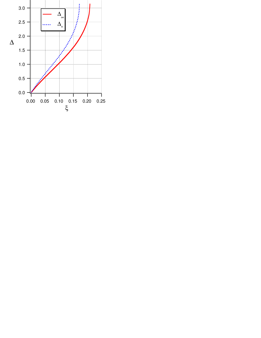
To determine the surface value of the radial coordinate we must solve equation (34) numerically for each set of values $(\xi,\eta)$ in the parameter space defined by (36). However, this can be avoided by observing that $\eta$ is an increasing function of $q$ for all $\xi$. Conversely, $q$ is an increasing function of $\eta$. Therefore, we can use $q$ as a parameter in place of $\eta$ to represent the sequence of stellar models. It follows that $q$ ranges from the minimal value $q=0$ corresponding to $\eta=\xi$ (see (36)) to a certain maximal value $q=q_{\infty}$ corresponding to $\eta=\eta_{\infty}=(1-4\xi^{2})/(4-\xi^{2})$. The value $q_{\infty}$ can only be determined implicitly by the equation $\sin(\xi q_{\infty})=\eta_{\infty}\sin q_{\infty}$. In the limit of small $\xi$ we find that $q_{\infty}$ will be close to $\pi$. Defining $\Delta:=\pi-q$ we have the relation

$$(1-4\xi^{2})\sin\Delta_{\infty}=(4-\xi^{2})\sin[\xi(\pi-\Delta_{\infty})]\ ,$$ (37)

for $\Delta_{\infty}$. This equation can be used to solve for $\Delta_{\infty}$ as a power series in $\xi$ with the result

$$\Delta_{\infty}=4\pi\xi-16\pi\xi^{2}+\pi(79+10\pi^{2})\xi^{3}+{\cal O}(\xi^{4})\ .$$ (38)

An issue here is the radius of convergence of this series. At this point we will content ourselves with the observation that for small enough $\xi$ the above series solution (38) gives a good approximate solution to (37). This is an indication that the radius of convergence is nonzero. For general $\xi$ it turns out to be more effective to solve (37) directly using a root finder routine. To obtain the value of $\Delta$ at the causal limit, $\Delta_{*}(\xi)$, we proceed in an analogous way observing first that $\eta_{*}=(1-5\xi^{2})/(5-\xi^{2})$, where $\eta_{*}$ is defined by letting the sound speed at the center be equal to the speed of light, $u_{\rm c}=1$. This leads to the equation

$$(1-5\xi^{2})\sin\Delta_{*}=(5-\xi^{2})\sin[\xi(\pi-\Delta_{*})]\ .$$ (39)

Again we solve this equation numerically using a root finding routine. The functions $\Delta_{\infty}(\xi)$ and $\Delta_{*}(\xi)$ are plotted in figure 5.

Figure 5: The function $\Delta_{\infty}(\xi)$ is plotted in the interval $0\leq\xi<\xi_{\infty}=(5-\sqrt{21})/2\approx 0.2087$. The function $\Delta_{*}(\xi)$ is plotted in the interval $0\leq\xi\leq\xi_{*}=3-2\sqrt{2}\approx 0.1716$. The models in the range $\xi_{*}<\xi<\xi_{\infty}$ have a superluminal sound speed at the center for all values of $\eta$.

Although the parameter $q$ is a good variable to describe sequences of models with $\xi\neq 0$ it is not a good variable in the limit $\xi\rightarrow 0$ since $q$ approaches the constant value $\pi$ in that limit. We wish to obtain a variable which works well also in the $\xi\rightarrow 0$ limit. Since $\eta$ is a good variable for the $\xi=0$ models we look for a new variable $\sigma$ which has the property $\sigma\rightarrow\eta$ as $\xi\rightarrow 0$. To that end we observe from (34) that $\eta=\xi q/(\pi-q)$ when $\xi\ll 1$. This motivates the definition $\sigma:=\xi q/(\pi-q)$. Then $\sigma\rightarrow\eta$ in the limit $\xi\rightarrow 0$ as required. Also, $\sigma$ is a nonnegative increasing function of $q$ and hence is also an increasing function of $\eta$. Finally we normalize $\sigma$ by defining $\hat{\sigma}:=\sigma/(4\sigma_{\infty})$ where $\sigma_{\infty}=\xi q_{\infty}/(\pi-q_{\infty})=\xi(\pi-\Delta_{\infty})/\Delta_{\infty}$. Then $\hat{\sigma}\rightarrow\eta$ as $\xi\rightarrow 0$ and $\hat{\sigma}_{\infty}=1/4$ for all $\xi$. We have

$$\hat{\sigma}=\frac{q\Delta_{\infty}}{4(\pi-q)(\pi-\Delta_{\infty})}\ ,$$ (40)

and solving for $q$ we obtain

$$q=\displaystyle\frac{4\pi(\pi-\Delta_{\infty})\hat{\sigma}}{\Delta_{\infty}+4(\pi-\Delta_{\infty})\hat{\sigma}}\ .$$ (41)

Expressing the causal limit in terms of the normalized parameter gives

$$\hat{\sigma}_{*}=\displaystyle\frac{\Delta_{\infty}(\pi-\Delta_{*})}{4\Delta_{*}(\pi-\Delta_{\infty})}\ .$$ (42)

3.1 Expressions for radius, mass and surface redshift

Figure 6: Contours of stellar radii are shown for the GB1 family. The radii are indicated in units of the characteristic length scale $\ell$. The solid contours are equidistant. The dotted contour has the value $r_{\rm s}/\ell=\pi/2\approx 1.57$. This is the minimum radius for Buchdahl’s gaseous models. The models with $\xi>0$ all have zero minimum radius reflecting their liquid-like equation of state. The causal limit as defined by (42) is indicated by the grey line. Models below that line are everywhere causal, $u<c$.

In the rest of the paper we set $R_{\pm}=0$. This implies that the model is regular throughout the interior of the star. To compute the radius we first use (5) to write

$$r=W(R)=\begin{cases}\displaystyle\frac{\ell}{2}\cdot\frac{\sqrt{1-\xi^{2}}}{\sqrt{1-\eta^{2}}}\,\left[\xi^{-1}\sin(\omega_{-}R)+\eta\sin(\omega_{+}R)\right]\ ,&\text{for $\xi\neq 0$ \ ,}\\[15.0pt] \displaystyle\frac{\ell}{2}\cdot\frac{1}{\sqrt{1-\eta^{2}}}[\omega_{+}R+\eta\sin(\omega_{+}R)]&\text{for $\xi=0$ \ .}\end{cases}$$ (43)

where $\ell:=1/\sqrt{\kappa a}$ is a characteristic length scale. Evaluating this expression at the surface we find

$$r_{\rm s}=W_{\rm s}=\begin{cases}\displaystyle\frac{\ell(1+\xi)\sqrt{1-\xi^{2}}\sin q\sin(\xi q)}{2\xi\sqrt{\sin^{2}q-\sin^{2}(\xi q)}}&\text{for $\xi\neq 0$ \ ,}\\[20.0pt] \displaystyle\frac{\pi\ell}{2\sqrt{1-\eta^{2}}}&\text{for $\xi=0$ \ .}\end{cases}$$ (44)

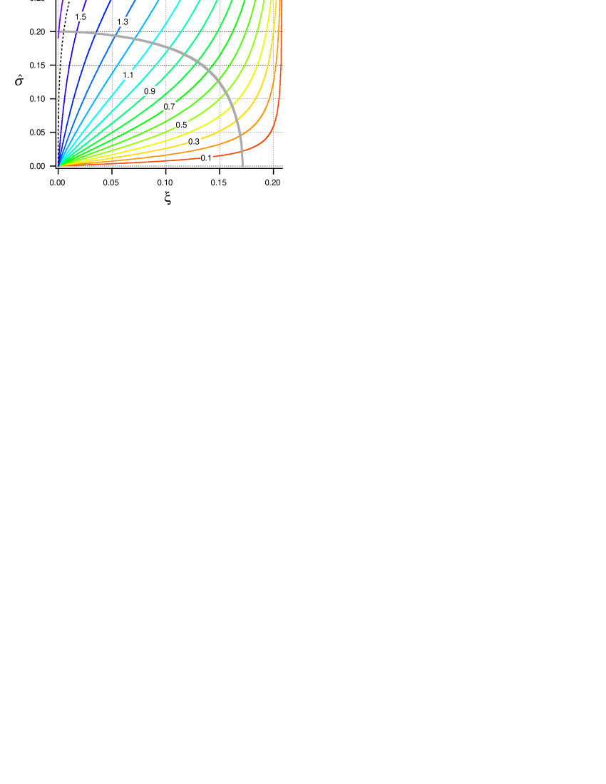
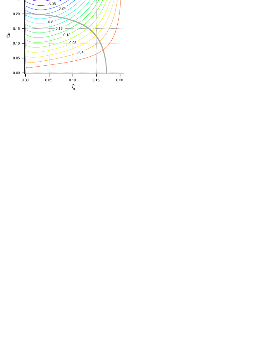
The radius is smallest in the limit $\eta\rightarrow\xi$ (or equivalently $q\rightarrow 0$ if $\xi\neq 0$). It is evident from (44) that for Buchdahl’s model the minimum radius is nonzero and is given by $(r_{\rm s})_{\rm min}=(\pi/2)\ell$. The models with $\xi>0$ on the other hand all have zero minimum radius as expected from their liquid-like equation of state. A contour plot of radii for the GB1 family is shown in figure 6.

Figure 7: Surface redshift contours are shown for all the GB1 models. The causal limit is indicated by the grey line. Models below that line are everywhere causal, $u<c$.

To compute the redshift we begin by writing down an expression for $\beta$. For that we need

$$W_{,R}=\begin{cases}(\cosh\zeta)\cos(\omega_{-}R)+(\sinh\zeta)\cos(\omega_{+}R)&\text{for $\xi\neq 0$ \ ,}\\[5.0pt] \cosh\zeta+(\sinh\zeta)\cos(\omega_{+}R)&\text{for $\xi=0$ \ ,}\end{cases}$$ (45)

leading to

$$(W_{,R})_{\rm s}=\begin{cases}(\cosh\zeta)\cos(\xi q)+(\sinh\zeta)\cos q=\sqrt{\displaystyle\frac{\sin[(1+\xi)q]}{\sin[(1-\xi)q]}}&\text{for $\xi\neq 0$\ ,}\\[10.0pt] e^{-\zeta}=\sqrt{\displaystyle\frac{1-\eta}{1+\eta}}&\text{for $\xi=0$ \ .}\end{cases}$$ (46)

This gives

$$\beta=\begin{cases}\textstyle{\frac{1}{2}}\left\{1-\displaystyle\frac{(1-\xi)\sin[(1+\xi)q]}{(1+\xi)\sin[(1-\xi)q]}\right\}&\text{for $\xi\neq 0$}\ ,\\[15.0pt] \displaystyle\frac{\eta}{1+\eta}&\text{for $\xi=0$}\ .\end{cases}$$ (47)

The expression for the redshift becomes

$$1+z_{\rm s}=\begin{cases}\sqrt{\displaystyle\frac{(1+\xi)\sin[(1-\xi)q]}{(1-\xi)\sin[(1+\xi)q]}}&\text{for $\xi\neq 0$}\ ,\\[20.0pt] \sqrt{\displaystyle\frac{1+\eta}{1-\eta}}&\text{for $\xi=0$}\ .\end{cases}$$ (48)

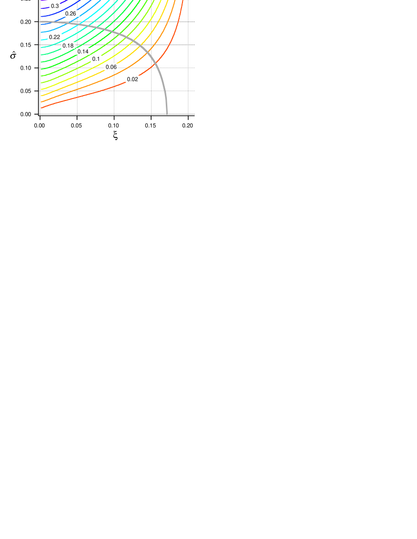
Comparison with the Doppler relation between redshift and velocity shows that for Buchdahl’s model $\eta$ is exactly equal to the corresponding velocity. The maximum equivalent velocity for Buchdahl’s model is therefore $v=\eta=1/4$ corresponding to a maximum redshift of $z_{\rm s}=\sqrt{5/3}-1\approx 0.291$. Restriction to causal models ($v=\eta<1/5$) gives a maximum redshift $z_{\rm s}=\sqrt{3/2}-1\approx 0.225$. A contour plot of surface redshifts for the GB1 family is shown in figure 7. The maximum value of the surface redshift can be computed numerically to be $z\approx 0.31$ which occurs for $\xi\approx 0.032$. The corresponding compactness parameter is $\alpha=1/\beta\approx 4.8$. Therefore there are no ultracompact models in the GB1 family. Turning now to the mass we find that it can be written as

$$M=\begin{cases}\displaystyle\frac{\ell(1+\xi)\sqrt{1-\xi^{2}}\sin q\sin(\xi q)}{4\xi\sqrt{\sin^{2}q-\sin^{2}(\xi q)}}\left\{1-\displaystyle\frac{(1-\xi)\sin[(1+\xi)q]}{(1+\xi)\sin[(1-\xi)q]}\right\}&\text{for $\xi\neq 0$ \ ,}\\[20.0pt] \displaystyle\frac{\pi\eta\ell}{2(1+\eta)\sqrt{1-\eta^{2}}}&\text{for $\xi=0$ \ .}\end{cases}$$ (49)

A contour plot of masses for the GB1 family is shown in figure 8.

Figure 8: Mass contours are shown for all the GB1 models. The masses are given in units of the characteristic length, $\ell$. The causal limit is indicated by the grey line. Models below that line are everywhere causal, $u<c$.

The central values of the pressure and energy density are given by

$$p_{\rm c}=\frac{4a(\eta^{2}-\xi^{2})}{(1-\xi^{2})(1+\eta)^{2}}\ ,\qquad\rho_{\rm c}=\frac{4a[\eta(2-3\eta)+\xi^{2}(3-2\eta)]}{(1-\xi^{2})(1+\eta)^{2}}\ .$$ (50)

The central values of the adiabatic index and sound speed are

$$\gamma_{\rm c}=\frac{2(1-\eta)(\eta+\xi^{2})^{2}}{(\eta^{2}-\xi^{2})[1-4\eta-(4-\eta)\xi^{2}]}\ ,\qquad u_{\rm c}=\frac{\eta+\xi^{2}}{1-4\eta-(4-\eta)\xi^{2}}\ .$$ (51)

The surface density is given by

$$\rho_{\rm s}=\frac{8a\xi}{(1+\xi)^{2}}\ .$$ (52)

3.2 Pressure and density profiles

The pressure and density functions are given in (6) as functions of $Z$. Expressing this function in terms of the normalized radial variable $\hat{R}:=R/R_{\rm s}$ we find

$$Z(\hat{R})=\frac{1-\phi(\hat{R})}{1+\phi(\hat{R})}\ ,$$ (53)

where

$$\phi(\hat{R}):=X/T=\begin{cases}\displaystyle\frac{\xi\sin(\xi q)\sin(q\hat{R})}{\sin q\sin(\xi q\hat{R})}\ .&\text{for $\xi\neq 0$ \ ,}\\[15.0pt] \displaystyle\frac{\eta\sin(\pi\hat{R})}{\pi\hat{R}}&\text{for $\xi=0$ \ .}\end{cases}$$ (54)

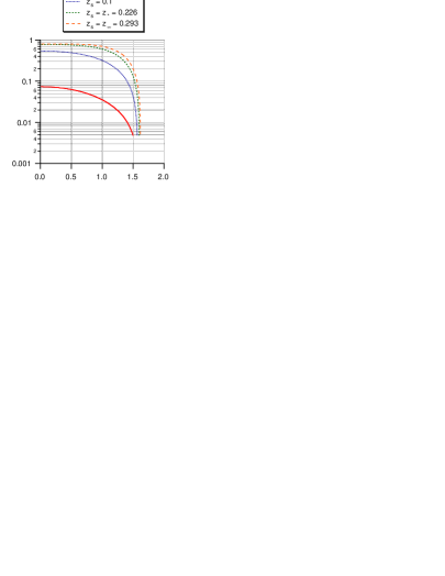
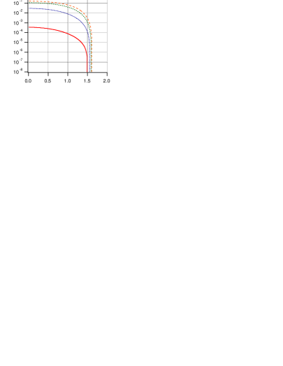
These formulas together with (6) give $p$ and $\rho$ as functions of $\hat{R}$. We wish to plot the pressure and density versus Schwarzschild’s radial variable which was given in equation (43). The result for Buchdahl’s model is shown in figure 9. A striking feature is the small variation in the radius. In going from a low mass Newtonian model with $z=0$ up to the most compact relativistic model with redshift $z=0.291$ the variation in the radius is only about 3%. The profiles for a representative of the type II GB1 family are shown in figure 10.

\psfrag{rhoB_bottom}{\Large$r/\ell$}\psfrag{rhoB_left}{\Large$\rho/\rho_{0}$}\includegraphics[width=211.26027pt]{rhoB.eps}

(a) Density profiles.

\psfrag{pB_bottom}{\Large$r/\ell$}\psfrag{pB_left}{\Large$p/p_{0}$}\includegraphics[width=211.26027pt]{pB.eps}

(b) Pressure profiles.

Figure 9: Density and pressure profiles for Buchdahl’s model ($\xi=0$). The density and pressure are given in units of $\rho_{0}=\kappa^{-1}\ell^{-2}$ and $p_{0}=\kappa^{-1}\ell^{-2}$. The profiles are given for four representative values of the surface redshift ranging from the mariginally relativistic, $z=0.01$, to the most extreme relativistic case, $z=z_{\infty}=\sqrt{5/3}-1\approx 0.291$. The radius takes values in the very narrow range, $\pi/2\leq r/\ell<2\pi/\sqrt{15}$, or approximately $1.571\leq r/\ell<1.622$.

(a) Density profiles.

(b) Pressure profiles.

Figure 10: Profiles for the type II GB1 models ($\xi=0.0006$). Axes and units are as in figure 9. The profiles are similar to those of the Buchdahl model except that the density is nonzero at the surface.

(a) Density profiles.

(b) Pressure profiles.

Figure 11: Profiles for type III GB1 models ($\xi=0.06$). Axes and units are as in figure 9.

(a) Density profiles.

(b) Pressure profiles.

Figure 12: Profiles for type IV GB1 models ($\xi=0.2$). Axes and units are as in figure 9.

4 Concluding remarks

We have described the 2-parameter GB1 family of exact spherically symmetric relativistic stellar models with a physically reasonable equation of state. One of the parameters represents the scaling invariance while the second parameter can be interpreted as a measure of the stiffness. By restricting the range of the stiffness parameter, one obtains a subfamily for which the sound speed is subluminal throughout the stellar interior. By varying the equation of state parameters it is possible to obtain a quite accurate fitting to the HW equation of state corresponding to the outer region of a neutron star.

Being a realistic model of a neutron star near the surface the GB1 family is a good candidate for a static limit of a rotating neutron star model. The main difficulty in trying to spin up a static perfect fluid model is to preserve the perfect fluid property. Technically this means that the Ricci tensor should have the correct algebraic type (Segré characteristic A1[(111),1)], see reference [22]) and in addition contain only a single arbitrary function. A recent result [23] seems to indicate that the Newman-Janis algorithm would always destroy the perfect fluid property. This could mean that a rotating perfect fluid model would not have a Kerr exterior.

The GB1 family is the only exact general physical SSS solution which is expressible in terms of elementary functions for all values of the integrations constants. For Schwarzschild’s interior solution, for example, only the regular models can be described in terms of elementary functions while the singular cases involve elliptic functions. It should be noted that the singular models have considerable physical interest. First they can be used in the regions outside the core of the star. Also, they are needed for obtaining a better understanding of the space of solutions as well as of the possibilities for global behaviour.

Appendix

Useful formulas

First some definitions:

$$\omega_{\pm}:=\sqrt{2(\delta\pm 1)\kappa a}\ ,\qquad\ell:=1/\sqrt{\kappa a}\ ,\qquad\xi:=\omega_{-}/\omega_{+}=\sqrt{\frac{\delta-1}{\delta+1}}\ .$$ (55)

We then have the following identities

$$\delta=\frac{1+\xi^{2}}{1-\xi^{2}}\ ,\qquad\delta+1=\frac{2}{1-\xi^{2}}\ ,\qquad\delta-1=\frac{2\xi^{2}}{1-\xi^{2}}\ ,\qquad\delta-\sqrt{\delta^{2}-1}=\frac{1-\xi}{1+\xi}\ ,$$ (56)

and

$$\omega_{+}{}^{-1}=\textstyle{\frac{1}{2}}\ell\sqrt{1-\xi^{2}}\ ,\qquad\omega_{-}{}^{-1}=\textstyle{\frac{1}{2}}\ell\xi^{-1}\sqrt{1-\xi^{2}}\ .$$ (57)

$$\eta:=\tanh\zeta\ ,\qquad e^{2\zeta}=\frac{1+\eta}{1-\eta}\ ,\qquad\cosh\zeta=\frac{1}{\sqrt{1-\eta^{2}}}\ ,\qquad\sinh\zeta=\frac{\eta}{\sqrt{1-\eta^{2}}}\ .$$ (58)

References

- [1] K. Rosquist, Class. Quantum Grav. 12, 1305 (1995).
- [2] W. Simon, Gen. Rel. Grav. 26, 97 (1994).
- [3] H. A. Buchdahl, Astrophys. J. 147, 310 (1967).
- [4] H. A. Buchdahl, Astrophys. J. 140, 1512 (1964).
- [5] K. Schwarzschild, Sitz. Preuss. Akad. Wiss. 424 (1916).
- [6] R. C. Tolman, Phys. Rev. 55, 364 (1939).
- [7] C. Uggla, R. T. Jantzen, and K. Rosquist, Phys. Rev. D 51, 5522 (1995).
- [8] B. K. Harrison, K. S. Thorne, M. Wakano, and J. A. Wheeler, Gravitation theory and gravitational collapse (University of Chicago Press, Chicago, USA, 1965).
- [9] K. Rosquist, Exact relativistic stellar models with liquid surface. II. Fitting the GB1 model to the Harrison-Wheeler equation of state, 1997, in preparation.
- [10] K. Rosquist, Exact relativistic stellar models with liquid surface. III. Generalizing Buchdahl’s polytrope, 1998, in preparation.
- [11] K. Rosquist, Trapped gravitational wave modes in stars with , 1998, E-print: gr-qc/9809033.
- [12] G. Neugebauer and R. Meinel, Astrophys. J. 414, L97 (1993).
- [13] E. T. Newman and A. I. Janis, J. Math. Phys. 6, 915 (1965).
- [14] L. Herrera and J. Jiménez, J. Math. Phys. 23, 2339 (1982).
- [15] S. P. Drake and R. Turolla, Class. Quantum Grav. 14, 1883 (1997).
- [16] W. D. Arnett and R. L. Bowers, Astrophys. J. Suppl. 33, 415 (1977).
- [17] J. T. Wheeler, Found. Phys. 25, 645 (1995).
- [18] CRC Handbook of Chemistry and Physics, 73 ed., edited by D. R. Lide (CRC Press, Boca Raton, Florida, 1992).
- [19] B. F. Schutz, A first course in general relativity (Cambridge University Press, Cambridge, U.K., 1985).
- [20] H. A. Buchdahl, Phys. Rev. 116, 1027 (1959).
- [21] L. Lindblom, Astrophys. J. 278, 364 (1984).
- [22] D. Kramer, H. Stephani, M. A. H. MacCallum, and E. Herlt, Exact Solutions of the Einstein Equations (VEB Deutscher Verlag der Wissenschaften, Berlin, GDR, 1980).
- [23] S. P. Drake and P. Szekeres, An explanation of the Newman-Janis algorithm, 1998, E-print: gr-qc/9807001.