Null Cones in Schwarzschild Geometry

Abstract

In this work we investigate aspects of light cones in a Schwarzschild geometry, making connections to gravitational lensing theory and to a new approach to General Relativity, the Null Surface Formulation. By integrating the null geodesics of our model, we obtain the light cone from every space-time point. We study three applications of the light cones. First, by taking the intersection of the light cone from each point in the space-time with null infinity, we obtain the light cone cut function, a four parameter family of cuts of null infinity, which is central to the Null Surface Formulation. We examine the singularity structure of the cut function. Second, we give the exact gravitational lens equations, and their specialization to the Einstein Ring. Third, as an application of the cut function, we show that the recently introduced coordinate system, the “pseudo-Minkowski” coordinates, are a valid coordinate system for the space-time.

1 Introduction

The purpose of this work is to develop a simple model space-time in which we study gravitational lensing and the light cone cuts of null infinity. These cuts are central to a recent reformulation of General Relativity known as the Null Surface Formulation [1, 2]. The model we consider consists of a Schwarzschild exterior region surrounding a spherically symmetric, static, constant density dust star.

The Null Surface Formulation makes explicit use of future null infinity, denoted by $\cal{I}^{+}$, which has the topology of $\mbox{\rm\bf R}\times S^{2}$. In an asymptotically simple space-time, $\cal{I}^{+}$ represents the future endpoints of all null geodesics and can be added as a boundary to the physical space-time through a process of conformal compactification [3]. The standard coordinates on $\cal{I}^{+}$ are the Bondi coordinates $(u,\theta,\phi)$, where $u$ labels the R part, and $\theta$ and $\phi$ label the sphere.

On $\cal{I}^{+}$, a light cone cut is the intersection of the light cone from a particular point in the interior with future null infinity. In Bondi coordinates on $\cal{I}^{+}$, the light cone cuts are given by a cut function,

$$u=Z(x^{a}_{\circ},\theta,\phi),$$ (1)

where for a fixed initial point, $x^{a}_{\circ}$, the cut is a deformed sphere, possibly with self-intersections and singularities. The crux of the Null Surface Formulation is that from the knowledge of the light cone cuts, Eq. (1), one can reconstruct all of the conformal information of the space-time.

The current paper explores the light cones from an arbitrary point in a Schwarzschild space-time surrounding a constant density, dust star. By integrating the null geodesics in an inverse radial coordinate $l~{}=~{}1/\sqrt{2}r$, we obtain parametric expressions for the future and past light cones of an initial point, $x^{a}_{\circ}$, in terms of a “distance” $l$, and two “directional” parameters which span the sphere of null directions at $x^{a}_{\circ}$. The intersection of the future light cone of an arbitrary initial point with null infinity gives the light cone cuts. In Section 3, we study the singularity structure of the cuts, explaining how the singularities are related to the formation of conjugate points on the light cone. We show in Section 4 that the equations for the past light cone obtained in Section 2 are, in fact, examples of exact lens equations. As a special case, we give the exact formula for the observation angle for an Einstein Ring. In the final section, we show that the “pseudo-Minkowski” coordinates, defined in [4], form a valid coordinate system for the entire space-time.

2 Integrating the Null Geodesics

To begin, we integrate the null geodesics of a Schwarzschild space-time with an interior constant density matter region. Since we eventually consider each geodesic’s limiting endpoint at $\cal{I}^{+}$ in order to obtain a cut function, we integrate the null geodesics using a conformal Schwarzschild metric which is regular at null infinity. The integration is performed using a “radial” parameter $l~{}=~{}1/(\sqrt{2}r)$, so that $l=0$ corresponds to the point at null infinity, while a finite $l>0$ will be a point in the interior.

The general form for a static, spherically symmetric metric with signature $(+,-,-,-)$ is given by

$$ds^{2}=f(r)dt^{2}-h(r)dr^{2}-r^{2}d\Omega^{2},$$ (2)

where $r^{2}d\Omega^{2}=r^{2}d\theta^{2}+r^{2}\sin^{2}\theta d\phi^{2}$ is the line element on the sphere. In our model, the functions $f(r)$ and $h(r)$ will be continuous, piecewise smooth functions for an exterior Schwarzschild region and an interior constant density dust solution with a radius $R$:

$$f(r)=\left(\frac{3}{2}\left(1-\frac{2M}{R}\right)^{\frac{1}{2}}-\frac{1}{2}\left(1-\frac{2Mr^{2}}{R^{3}}\right)^{\frac{1}{2}}\right)^{2}\equiv f_{int},\quad r<R,$$

$$f(r)=1-\frac{2M}{r}\equiv f_{ext},\quad\quad r>R,$$

$$h(r)=\frac{1}{1-\frac{2Mr^{2}}{R^{3}}}\equiv h_{int},\quad\quad r<R,$$

$$h(r)=\frac{1}{1-\frac{2M}{r}}\equiv h_{ext},\quad\quad r>R.$$ (3)

We assume that the radius of the interior region extends beyond the $r=3M$ unstable circular orbit for null geodesics, ensuring that the space-time is asymptotically simple. Working in a retarded null coordinate, $u=t-\int dr\sqrt{h(r)/f(r)}$, and the inverted radial coordinate, $l~{}=~{}1/(\sqrt{2}r)$, a conformally rescaled version of the metric, Eq. (2), which is regular at null infinity, is

$$d\hat{s}^{2}=4l^{2}~{}f(l)~{}du^{2}-4\sqrt{k(l)}du~{}dl-d\Omega^{2},$$ (4)

where $r$ is replaced in terms of the variable $l$ and $k(l)$ is given by

$$k(l)=f(l)~{}h(l).$$

It is convenient to integrate the null geodesics first in a plane, and then to use the spherical symmetry to rotate the solution to an arbitrary orientation. The restriction we employ is to take a particular initial point, ${\tilde{x}}^{a}_{\circ}$, lying on the $-\hat{z}$ axis,

$${\tilde{x}}^{a}_{\circ}=(u_{\circ},l_{\circ},\tilde{\theta}_{\circ}=\pi,\tilde{\phi}_{\circ}=0),$$

and the geodesics as lying in the $\hat{x}$-$\hat{z}$ plane. To define the $\hat{x}$-$\hat{z}$ plane, one usually allows $\theta$ to range from $0$ to $\pi$ and has $\phi=0$ or $\pi$. In order to facilitate our discussion, we will not use this convention. Instead, we require that $\phi=0$ and allow a variable, $\Theta$, to range from $0$ to $2\pi$. In terms of the variables $(u,l,\Theta)$, a Lagrangian corresponding to the conformal metric is

$${\cal L}=2l^{2}~{}f(l)~{}{\dot{u}}^{2}-2\sqrt{k(l)}~{}{\dot{u}}~{}{\dot{l}}-\frac{1}{2}{\dot{\Theta}}^{2},$$ (5)

where dots indicate derivatives with respect to an affine parameter $\tau$. The geodesic equations are

$$\frac{d}{d\tau}(2l^{2}~{}f(l)~{}\dot{u}-\sqrt{k(l)}~{}\dot{l})=0,$$

$$\frac{d}{d\tau}(-\sqrt{k(l)}~{}\dot{u})-(2l~{}f(l)~{}\dot{u}^{2}+l^{2}~{}f^{\prime}(l)~{}\dot{u}^{2})+\frac{\dot{u}~{}\dot{l}}{2\sqrt{k(l)}}(k^{\prime}(l))=0,$$

$$\frac{d}{d\tau}\dot{\Theta}=0,$$ (6)

with primes denoting derivatives with respect to $l$. To solve for null geodesics, we impose the null condition on the Lagrangian,

$${\cal L}=2l^{2}~{}f(l)~{}{\dot{u}}^{2}-2\sqrt{k(l)}~{}{\dot{u}}~{}{\dot{l}}-\frac{1}{2}{\dot{\Theta}}^{2}=0,$$ (7)

and use this equation and the first and third geodesic equations as independent equations for $(u,l,\Theta)$. After finding some trivial first integrals and rearranging, independent equations for null geodesics can be written as

$$\dot{u}={{1+\sqrt{k(l)}~{}\dot{l}}\over{2l^{2}~{}f(l)}},$$

$$\dot{l}=\pm\sqrt{{{1-b^{2}~{}l^{2}~{}f(l)}\over{k(l)}}}\equiv\pm\sqrt{A(l)},$$

$$\dot{\Theta}=b.$$ (8)

In these equations the sign of $\dot{l}$ indicates whether the geodesic is incoming (positive) or outgoing (negative), and the parameter $b$ is a free integration parameter labeling the initial direction of the geodesic. In Appendix A, we show how the parameter $b$ is related to the initial direction of the null geodesic.

In integrating the equations, geodesics which are initially outgoing will have $b$ values ranging from zero, corresponding to a ray traveling radially outward, to some maximum value $b_{m}$, for which the geodesic is initially tangent to a sphere of radius $r_{\circ}=1/(\sqrt{2}l_{\circ})$. The value of $b_{m}$ is the value of $b$ for which $\dot{l}=0$ at the point $l=l_{\circ}$:

$$b_{m}=\frac{1}{l_{\circ}\sqrt{f(l_{\circ})}}.$$ (9)

For geodesics which are initially incoming, the range in $b$ will be from $b_{m}$ back down to zero. The value of $l$ will increase until reaching some maximum value, $l=l_{b}$, which is a minimum $r$ value. The value of $l_{b}$ is the single (real) root of the equation, $\dot{l}=0$, or the root of:

$$1-b^{2}~{}l_{b}^{2}~{}f(l_{b})=0.$$ (10)

At $l_{b}$, $\dot{l}$ changes sign, and the geodesics will head out to infinity.

It is convenient to reparametrize the equations of motion, Eqs. (8), using $l$ instead of the affine parameter, and to express the solution to the null geodesic equations in terms of integrals over $l$. In terms of these integrals, geodesics on the light cone connecting the initial point, ${\tilde{x}}_{\circ}^{a}=(u_{\circ},l_{\circ},\theta_{\circ}~{}=~{}\pi,\phi_{\circ}~{}=~{}0)$, with the final point, $x^{a}=(u,~{}l,~{}\Theta,~{}\phi~{}=~{}0)$, are given by

$$u=u(u_{\circ},l_{\circ},l,b)=u_{\circ}+(-1)^{\epsilon}\int_{l_{\circ}}^{l}~{}dl^{\prime}~{}\left(\pm{{1\pm\sqrt{k(l^{\prime})~{}A(l^{\prime})}}\over{\sqrt{A(l^{\prime})}(2l^{\prime 2}~{}f(l^{\prime}))}}\right),$$

$$\Theta=\Theta(l_{\circ},l,b)=\pi-\int_{l_{\circ}}^{l}~{}dl^{\prime}~{}\left(\pm\frac{b}{\sqrt{A(l^{\prime})}}\right),$$

$$\phi=0,$$ (11)

where the integrals are defined piecewise over the various segments in $f$ and $k$, and the appropriate signs are chosen if the geodesics are incoming ($+$) or outgoing ($-$). The future light cone is given by $\epsilon=0$, and the past light cone by $\epsilon=1$.

The full solution to the null geodesic equations is obtained by performing a rigid rotation of the spatial plane defined by the path of this geodesic and the $\hat{z}$ axis, to an arbitrary orientation. Due to spherical symmetry, the light cone for an arbitrary point will be axially symmetric about the spatial line connecting that point and the spatial origin (defined by $r=0$). We will call the angle of revolution about the axis of symmetry $\gamma$; the angle $\gamma$ essentially defines an orientation of the spatial plane containing the geodesic and the axis of symmetry. (In the case that the initial point lies on the $-\hat{z}$ axis, $\gamma$ is simply the angle $\phi$.) To obtain the full light cone from an arbitrary initial point, we need to rotate the solution that is symmetric about the $\hat{z}$ axis over to the axis of symmetry defined by the arbitrary point. We can think of this as rotating the particular initial point ${\tilde{x}}_{\circ}^{a}~{}=~{}(u_{\circ},~{}l_{\circ},~{}\theta_{\circ}~{}=~{}\pi,~{}\phi_{\circ}~{}=~{}0)$ to the general initial point $x^{a}_{\circ}~{}=~{}(u_{\circ},~{}l_{\circ},~{}\theta_{\circ},~{}\phi_{\circ})$ and allowing the orientation parameter $\gamma$ to take any value between $0$ and $2\pi$. This rotation is explicitly performed in Appendix B.

It is often convenient to use complex stereographic coordinates, defined by

$$\zeta=\cot{\frac{\theta}{2}}e^{i\phi},\quad\quad\bar{\zeta}=\cot{\frac{\theta}{2}}e^{-i\phi},$$ (12)

instead of the angular coordinates $\theta$ and $\phi$. Throughout this paper we freely switch back and forth between the two coordinate systems. An arbitrary initial point is given in stereographic coordinates by $x^{a}_{\circ}~{}=~{}(u_{\circ},~{}l_{\circ},~{}\zeta_{\circ},~{}\bar{\zeta}_{\circ})$.

The full light cone, obtained by using the rotation of the solutions of the null geodesic equations in the $\hat{x}$-$\hat{z}$ plane to an arbitrary initial point and orientation given in Appendix B, are expressed parametrically in terms of the parameter $l$ as

$$u=u(u_{\circ},l_{\circ},l,b)=u_{\circ}+(-1)^{\epsilon}\int_{l_{\circ}}^{l}~{}dl^{\prime}~{}\left(\pm{{1\pm\sqrt{k(l^{\prime})~{}A(l^{\prime})}}\over{\sqrt{A(l^{\prime})}(2l^{\prime 2}~{}f(l^{\prime}))}}\right),$$

$$\zeta(l_{\circ},\zeta_{\circ},\bar{\zeta}_{\circ},l,b,\gamma)=\left(\frac{\zeta_{\circ}}{\bar{\zeta}_{\circ}}\right)^{\frac{1}{2}}\left(\frac{e^{\frac{i}{2}\gamma}\cot{\frac{\Theta(l,l_{\circ},b)}{2}}+\sqrt{\zeta_{\circ}\bar{\zeta}_{\circ}}e^{-\frac{i}{2}\gamma}}{-\sqrt{\zeta_{\circ}\bar{\zeta}_{\circ}}e^{\frac{i}{2}\gamma}\cot{\frac{\Theta(l,l_{\circ},b)}{2}}+e^{-\frac{i}{2}\gamma}}\right),$$

$$\bar{\zeta}(l_{\circ},\zeta_{\circ},\bar{\zeta}_{\circ},l,b,\gamma)=\left(\frac{\bar{\zeta}_{\circ}}{\zeta_{\circ}}\right)^{\frac{1}{2}}\left(\frac{e^{-\frac{i}{2}\gamma}\cot{\frac{\Theta(l,l_{\circ},b)}{2}}+\sqrt{\zeta_{\circ}\bar{\zeta}_{\circ}}e^{\frac{i}{2}\gamma}}{-\sqrt{\zeta_{\circ}\bar{\zeta}_{\circ}}e^{-\frac{i}{2}\gamma}\cot{\frac{\Theta(l,l_{\circ},b)}{2}}+e^{\frac{i}{2}\gamma}}\right),$$ (13)

where $\Theta(l,l_{\circ},b)$ is given by the integral in Eq. (11),

$$\Theta=\Theta(l_{\circ},l,b)=\pi-\int_{l_{\circ}}^{l}~{}dl^{\prime}~{}\left(\pm\frac{b}{\sqrt{A(l^{\prime})}}\right),$$ (14)

and the convention for $\epsilon$ and signs are taken as before.

Eqs. (13) represent the entire future and past light cones for an arbitrary point in the space-time. The light cones are given in terms of two parameters, $(b,~{}\gamma)$, which span the sphere of initial null directions at the initial point $x^{a}_{\circ}$. We note that the $u$ coordinate does not depend on $\gamma$ due to the axial symmetry of the light cone.

3 Light Cone Cuts and their Singularities

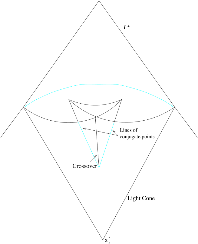
Figure 1: The light cone of a point which has formed conjugate points in its future. The crossover line represents points in the space-time where Einstein Rings are observed, while the line of caustics are stable singularities conjugate to the initial point.

While the light cone from an arbitrary point in Minkowski space is always smooth, light cones in an asymptotically simple space-time have, in general, self-intersections and several different kinds of singularities. These singularities are directly related to the formation of conjugate points along null geodesics. A pictorial representation of a light cone with singularities is given in Figure 1. Since the light cone cut function is the intersection of the future light cone with null infinity, it inherits the singularity structure of the light cone. In this section, we study the cut function in our model as a representative example of the Null Surface Formulation.

A parametric version of the cut function is obtained by setting the values of $l$ and $\epsilon$ to zero in Eqs. (13):

$$u_{\infty}(u_{\circ},l_{\circ},b)=u_{\circ}+\int_{l_{\circ}}^{0}~{}dl^{\prime}~{}\left(\pm{{1\pm\sqrt{k(l^{\prime})~{}A(l^{\prime})}}\over{\sqrt{A(l^{\prime})}(2l^{\prime 2}~{}f(l^{\prime}))}}\right),$$ (15)

$$\zeta_{\infty}(l_{\circ},\zeta_{\circ},\bar{\zeta}_{\circ},b,\gamma)=\left(\frac{\zeta_{\circ}}{\bar{\zeta}_{\circ}}\right)^{\frac{1}{2}}\left(\frac{e^{\frac{i}{2}\gamma}\cot{\frac{\Theta(l_{\circ},b)}{2}}+\sqrt{\zeta_{\circ}\bar{\zeta}_{\circ}}e^{-\frac{i}{2}\gamma}}{-\sqrt{\zeta_{\circ}\bar{\zeta}_{\circ}}e^{\frac{i}{2}\gamma}\cot{\frac{\Theta(l_{\circ},b)}{2}}+e^{-\frac{i}{2}\gamma}}\right),$$ (16)

$$\bar{\zeta}_{\infty}(l_{\circ},\zeta_{\circ},\bar{\zeta}_{\circ},b,\gamma)=\left(\frac{\bar{\zeta}_{\circ}}{\zeta_{\circ}}\right)^{\frac{1}{2}}\left(\frac{e^{-\frac{i}{2}\gamma}\cot{\frac{\Theta(l_{\circ},b)}{2}}+\sqrt{\zeta_{\circ}\bar{\zeta}_{\circ}}e^{\frac{i}{2}\gamma}}{-\sqrt{\zeta_{\circ}\bar{\zeta}_{\circ}}e^{\frac{-i}{2}\gamma}\cot{\frac{\Theta(l_{\circ},b)}{2}}+e^{\frac{i}{2}\gamma}}\right),$$ (17)

where the function $\Theta(l_{\circ},b)$ is given by

$$\Theta(l_{\circ},b)=\pi-\int_{l_{\circ}}^{0}~{}dl^{\prime}~{}\left(\pm\frac{b}{\sqrt{A(l^{\prime})}}\right).$$ (18)

If it were possible to invert the pair of equations, Eqs. (16) and (17), for $b$ and $\gamma$, obtaining the functions

$$\gamma=G(\zeta_{\infty},\bar{\zeta}_{\infty},\zeta_{\circ},\bar{\zeta}_{\circ},l_{\circ}),$$ (19)

and

$$b=B(\zeta_{\infty},\bar{\zeta}_{\infty},\zeta_{\circ},\bar{\zeta}_{\circ},l_{\circ}),$$ (20)

one could produce the full cut function in the form of Eq. (1),

$$u=Z(x^{a}_{\circ},\zeta,\bar{\zeta}),$$

by inserting the solution for $b$ in terms of $(\zeta,\bar{\zeta})$ from Eq. (20) into the $u_{\infty}$ solution, Eq. (15).

While $\zeta_{\infty}(l_{\circ},~{}\zeta_{\circ},~{}\bar{\zeta}_{\circ},~{}b,~{}\gamma)$, and $\bar{\zeta}_{\infty}(l_{\circ},~{}\zeta_{\circ},~{}\bar{\zeta}_{\circ},~{}b,~{}\gamma)$ are single valued in $b$, they will not, in general, have unique inverses—more than one initial direction acquires the same value of $\zeta$ or $\bar{\zeta}$ at $\cal{I}+$. This implies that there are singularities in the cut function itself and that the global inversion of Eqs. (16) and (17) for $b$ and $\gamma$ will be impossible. In such a case, we will not be able to find an explicit cut function in the form of Eq. (1), but will be forced to work with the cut function in a parametric form.

In a sense, singularities in the light cone cuts are places where the Null Surface Formulation undergoes technical difficulties—a natural coordinate system used in the theory is not well defined at these points. We now believe that these difficulties can be overcome by using a particular parametric representation the cut function. A primary interest here is to study the singularities in the cut function.

There is a complete classification of the stable singularities of the cut function which can be applied to our model, due to Arnol’d and his collaborators [5, 6]. A stable singularity is one which does not disappear under small perturbations. For two dimensional surfaces, such as the light cone cuts obtained by fixing the initial point in the cut function, there are only two types of stable singularities. These are the cusp ridge and the swallowtail. Due to high level of symmetry in our model, any cut function must be axially symmetric. This means that, although the cut function is a two dimensional surface, it can be represented by a one dimensional curve whose revolution about some axis gives the cut function. For a one dimensional curve, the only stable singularity is a cusp, which implies that we will not see swallowtail singularities in our model.

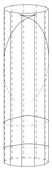
Figure 2: Three cut functions with one dimension suppressed ($S\times\mbox{\rm\bf R}$). As the initial radial position moves away from the spatial center smooth cuts give way to cuts with singularities.

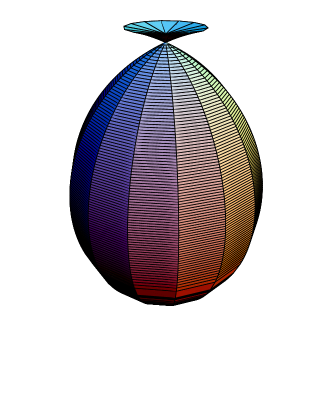
Figure 3: A cusp ridge appears on the light cone cut from an initial point sufficiently far away from the center of the space-time. Near $\cal{I}^{+}$, the intersection of the light cone of this initial point with a time-like surface would look similar to this cut, except that the “umbrella” at the top of the cut would be inside the main body of the wavefront.

In Figure 2, we give plots of three cut functions, suppressing the axially symmetric dimension, for three different values of the initial radial position, $l_{\circ}$. These figures show that singularities appear as the initial point moves away from the spatial center of the space-time. A smooth cut of null infinity, corresponding to a cut from the light cone of a point close to the center of the space-time, will be a smooth sphere-like surface. Due to the axial symmetry, a cut with singularities will have a circular cusp ridge and a single crossover point. Figure 3 gives a pictorial representations of a singular cut.

Because the cusp ridge singularity in our cut function is stable, it represents a generic possibility for a cut function in a general space-time. Specifically, this singularity will remain if one makes a small perturbation of the metric away from a Schwarzschild metric. The crossover point along the cut function is an unstable singularity, arising from the high degree of symmetry in the Schwarzschild case, and is directly related to Einstein’s Rings, the astronomical phenomenon where a spherical lens causes lensing in a uniform circular shape [7]. We discuss the rings in the next section on gravitational lensing.

The singularities in the cut function represent points which are conjugate to the initial point $x^{a}_{\circ}$. For a fixed $x^{a}_{\circ}$, we can think of the parametric equations for the cut function, Eqs. (15), (16), and (17), as a map between the initial directions of the geodesics at the initial point and the final position $(u_{\infty},\zeta_{\infty},\bar{\zeta}_{\infty})$ at $\cal{I}^{+}$. One way to find the points of $\cal{I}^{+}$ which are conjugate to the initial point $x^{a}_{\circ}$ is to find the points at $\cal{I}^{+}$ for which the Jacobian matrix expressing the mapping,

$$J=\pmatrix{\frac{\partial u_{\infty}}{\partial b}&\frac{\partial u_{\infty}}{\partial\gamma}\cr\frac{\partial\zeta_{\infty}}{\partial b}&\frac{\partial\zeta_{\infty}}{\partial\gamma}\cr\frac{\partial\bar{\zeta}_{\infty}}{\partial b}&\frac{\partial\bar{\zeta}_{\infty}}{\partial\gamma}\cr},$$ (21)

drops in rank [9]. For this to occur, all three $2\times 2$ determinants must be zero.

With no loss in generality, we consider the cut function of an initial point on the $-\hat{z}$ axis. In this case, the cut function is obtained by setting the final value of $l$ in Eq. (11) to zero, and restoring the rotational degree of freedom by setting $\gamma=\phi_{\infty}$. Thus, the cut function for an initial point on the $-\hat{z}$ axis is written in terms of the coordinates $(u_{\infty},~{}\theta_{\infty},~{}\phi_{\infty})$ as

$$u_{\infty}(u_{\circ},l_{\circ},b)=u_{\circ}+\int_{l_{\circ}}^{0}~{}dl^{\prime}~{}\left(\pm{{1\pm\sqrt{k(l^{\prime})~{}A(l^{\prime})}}\over{\sqrt{A(l^{\prime})}(2l^{\prime 2}~{}f(l^{\prime}))}}\right),$$

$$\theta_{\infty}(l_{\circ},b)=\pi-\int_{l_{\circ}}^{0}~{}dl^{\prime}~{}\left(\pm\frac{b}{\sqrt{A(l^{\prime})}}\right),$$

$$\phi_{\infty}=\gamma.$$ (22)

In this case, the Jacobian matrix corresponding to Eq. (21) is given by

$$J=\pmatrix{\frac{\partial u_{\infty}}{\partial b}&0\cr\frac{\partial\theta_{\infty}}{\partial b}&0\cr 0&1\cr}.$$ (23)

It is clear that for the Jacobian to drop rank we must have

$$\frac{\partial u_{\infty}}{\partial b}=0,$$ (24)

and

$$q\equiv\frac{d\theta_{\infty}}{db}=0,$$ (25)

A combination of numerical and analytic calculations shows that these two conditions are satisfied simultaneously only at the cusp ridge shown in the figures, and hence the cusps on the cut function are conjugate points to the initial point.

An alternative way of deducing the singular points is to consider the first and second derivatives of $u_{\infty}$ with respect to $\theta_{\infty}$. For a cusp singularity, the first derivatives are always finite, while the second derivatives diverge. Working parametrically in $b$, these derivatives are

$$\frac{\partial u_{\infty}}{\partial\theta_{\infty}}=\frac{\frac{\partial u_{\infty}}{\partial b}}{\frac{\partial\theta_{\infty}}{\partial b}},$$

and,

$$\frac{\partial^{2}u_{\infty}}{\partial\theta_{\infty}^{2}}=\left(\frac{\partial\theta_{\infty}}{\partial b}\right)^{-2}\left[\frac{\partial^{2}u_{\infty}}{\partial b^{2}}-\frac{\partial u_{\infty}}{\partial\theta_{\infty}}\frac{\partial^{2}\theta_{\infty}}{\partial b^{2}}\right].$$ (26)

Numerical computation shows that the first derivative is finite and non-zero along the cusps in the light cone cut. As written, the second derivative is indeterminant along the cusps since the term in square brackets is zero there. Applying L’Hôspital’s rule, one sees that the second derivative actually diverges as $q^{-1}$.

As a final note on the cusp singularities, we list the behavior of several important quantities in the Null Surface Formulation as one approaches the cusps along the cut function. All of these quantities are computed as derivatives of the cut function with respect to the complex stereographic coordinates $\zeta$ and $\bar{\zeta}$, and have been computed in this model parametrically for initial points along the $-\hat{z}$ axis. These derivatives are denoted by ð and $\bar{\mbox{\dh}}$ [8]. In terms of $q$, which approaches zero as one approaches the cusp, the behavior of some important quantities of interest are listed below for $u_{\infty}~{}=~{}Z(x_{\circ}^{a},\zeta,\bar{\zeta})$.

Quantity	Behavior
$\omega=\mbox{\dh}Z$	regular
$\Lambda={\mbox{\dh}}^{2}Z$	$q^{-1}$
$R=\bar{\mbox{\dh}}\mbox{\dh}Z$	$q^{-1}$
$|\Lambda,_{1}|=|\frac{d\Lambda}{dR}|$	$1$
$\Omega^{2}=g^{ab}Z,_{a}\bar{\mbox{\dh}}\mbox{\dh}Z,_{b}$	$q^{-2}$

4 Gravitational Lensing Equations

An important goal of gravitational lensing theory is to construct lens equations which give the position of sources in terms of directions seen by an observer and distances to the source. Typically, lens equations are obtained via approximations on the kinematics of the null geodesics of the source [7].

Recently, a way to produce completely general, exact lensing equations has been found, and a paper is being prepared which develops gravitational lensing theory from this perspective [9]. Our model provides an explicit example of such a formulation. In this section we give exact lensing equations for the Schwarzschild space-time with a constant density dust interior region, and show that our exact equations reduce to standard approximate lens equations. In the special case that the source, lens, and observer are spatially colinear, we give an exact expression for the observation angle in an Einstein Ring.

In Section 2, we derived the future and past light cones of an arbitrary point in the space-time. Recall that a lens equation should express the location of the source in terms of some “distance” from the observer, and the directions which the observer views the geodesics on the past light cone. The equations of the past light cone, Eqs. (13), are such a set of equations. In these equations, the observed directions are given by the parameters $(b,\gamma)$, and $l$ gives the “distance.” Hence, exact lens equations for our model are

$$\zeta(l_{\circ},\zeta_{\circ},\bar{\zeta}_{\circ},l,b^{\ast},\gamma^{\ast})=\left(\frac{\zeta_{\circ}}{\bar{\zeta}_{\circ}}\right)^{\frac{1}{2}}\left(\frac{e^{\frac{i}{2}\gamma^{\ast}}\cot{\frac{\Theta(l,l_{\circ},b^{\ast})}{2}}+\sqrt{\zeta_{\circ}\bar{\zeta}_{\circ}}e^{-\frac{i}{2}\gamma^{\ast}}}{-\sqrt{\zeta_{\circ}\bar{\zeta}_{\circ}}e^{\frac{i}{2}\gamma^{\ast}}\cot{\frac{\Theta(l,l_{\circ},b^{\ast})}{2}}+e^{-\frac{i}{2}\gamma^{\ast}}}\right),$$

$$\bar{\zeta}(l_{\circ},\zeta_{\circ},\bar{\zeta}_{\circ},l,b^{\ast},\gamma^{\ast})=\left(\frac{\bar{\zeta}_{\circ}}{\zeta_{\circ}}\right)^{\frac{1}{2}}\left(\frac{e^{-\frac{i}{2}\gamma^{\ast}}\cot{\frac{\Theta(l,l_{\circ},b^{\ast})}{2}}+\sqrt{\zeta_{\circ}\bar{\zeta}_{\circ}}e^{\frac{i}{2}\gamma^{\ast}}}{-\sqrt{\zeta_{\circ}\bar{\zeta}_{\circ}}e^{\frac{-i}{2}\gamma^{\ast}}\cot{\frac{\Theta(l,l_{\circ},b^{\ast})}{2}}+e^{\frac{i}{2}\gamma^{\ast}}}\right),$$ (27)

with

$$\Theta(l,l_{\circ},b^{\ast})=\pi-\int_{l_{\circ}}^{l}~{}dl^{\prime}~{}\left(\pm\frac{b^{\ast}~{}\sqrt{k(l^{\prime})}}{\sqrt{1-{b^{\ast}}^{2}~{}l^{\prime 2}~{}f(l^{\prime})}}\right).$$

In these lens equations, the spatial location of the source is the point $(l,\zeta,\bar{\zeta})$. For an observer at the point $(l_{\circ},\zeta_{\circ},\bar{\zeta}_{\circ})$, the observed directions of the geodesic on the past null cone are given by the particular values of $(b,\gamma)$ which connect the source and the observer, denoted as $(b^{\ast},\gamma^{\ast})$. There may, in fact, be more than one set of values for $(b^{\ast},\gamma^{\ast})$, as the process of focusing may produce more than one “image.”

Due to spherical symmetry, any observer may be considered as lying on the $-\hat{z}$ axis, and the source may be taken as lying in the $\hat{x}$-$\hat{z}$ plane. We are interested in the case where the lens is situated between the observer and the source, and when the rays do not pass through the interior region of the star. In this case, the lens equations, Eqs. (27), reduce to the single equation for $\Theta$ which was found in Eq. (11):

$$\Theta(l_{\circ},l,b^{\ast})=\pi-\int_{l_{\circ}}^{l}~{}dl^{\prime}~{}\left(\pm\frac{b^{\ast}}{\sqrt{1-{b^{\ast}}^{2}~{}l^{\prime 2}~{}f(l^{\prime})}}\right).$$ (28)

This lens equation specifies the location of the source in terms of the observed direction of the geodesic, $b^{\ast}$, and a “distance,” $l$, to the source.

In Appendix A, we find the relationship between the angle at which a null geodesic crosses the $\hat{z}$ axis, the parameter $b$, and a position $l$. In the lensing case, this “observation angle,” denoted by $\psi_{obs}$, is related to the observer position, $l_{\circ}$, and the observed direction, $b^{\ast}$, by

$$b^{\ast}=\frac{\sin{\psi_{obs}}}{l_{\circ}~{}\sqrt{f(l_{\circ})}}.$$ (29)

By replacing $b^{\ast}$ by $\psi_{obs}$ in the lens equation, Eq. (28), the lens equation takes a more conventional form, where the direction parameter is the actual observation angle:

$$\Theta(l_{\circ},l,b^{\ast})=\pi-\frac{\sin{\psi_{obs}}}{l_{\circ}~{}\sqrt{f(l_{\circ})}}~{}\int_{l_{\circ}}^{l}~{}dl^{\prime}~{}\left(\pm\frac{1}{\sqrt{1-\frac{\sin^{2}{\psi_{obs}}~{}l^{\prime 2}~{}f(l^{\prime})}{l_{\circ}^{2}~{}f(l_{\circ})}}}\right).$$ (30)

A typical approximate lens equation for the Schwarzschild model [7] is

$$\beta=\psi-\frac{2R_{S}~{}D_{LS}}{D_{L}~{}D_{S}~{}\psi}.$$ (31)

In this approximation, $\beta$ is the Euclidean angle between the source and the center of the space-time, and $R_{S}=2M$ is the Schwarzschild radius. The Euclidean distances between the source and lens, source and observer, and lens and observer, are given by $D_{LS}$, $D_{S}$, and $D_{L}$ respectively. Figure 4 shows the case under consideration. We now show that our lens equation, Eq. (30) or Eq. (28), reduces to the approximate formula, Eq. (31), under appropriate approximations.

Taking into account the correct signs for incoming and outgoing rays, the right hand side of Eq. (28) can be written as

$$\Theta=\pi-\Delta(M,b^{\ast},l_{\circ},l),$$ (32)

where

$$\Delta = 2~{}\int_{l_{\circ}}^{l_{b}}~{}\frac{b^{\ast}~{}dl^{\prime}}{\sqrt{2\sqrt{2}M~{}{b^{\ast}}^{2}~{}l^{\prime 3}-{b^{\ast}}^{2}~{}l^{\prime 2}+1}}$$ (33)

$${}+\int_{l}^{l_{\circ}}~{}\frac{b^{\ast}~{}dl^{\prime}}{\sqrt{2\sqrt{2}M~{}{b^{\ast}}^{2}~{}l^{\prime 3}-{b^{\ast}}^{2}~{}l^{\prime 2}+1}}.$$

Here, $l_{\circ}$ is the position of the observer, $l$ is the position of the source, and $l_{b}$ is the value of $l$ for which the geodesic comes closest to the lens, attained when $\dot{l}=0$. The maximum $l$ value, $l_{b}$, is, from Eq. (10), the solution of the equation

$$1-{b^{\ast}}^{2}~{}l_{b}^{2}+2\sqrt{2}M~{}{b^{\ast}}^{2}~{}l_{b}^{3}=0.$$ (34)

For convenience, we assume that the source is closer to the lens than the observer, so that $l>l_{\circ}$. To proceed, we assume that the dimensionless quantities $M~{}l\equiv\epsilon$ and $M~{}l_{\circ}<\epsilon$ are small and make a Taylor series expansion of $\Delta$ in terms of $\epsilon$:

$$\Delta(\epsilon,b^{\ast},l_{\circ},l)=\Delta(\epsilon=0,b^{\ast},l_{\circ},l)+\epsilon\left[\frac{\partial\Delta}{\partial\epsilon}\right]_{\epsilon=0}\equiv\Delta_{\circ}+\Delta_{1}.$$

To compute $\Delta_{\circ}$, we evaluate Eq. (33) at $\epsilon=M=0$. This implies that $l_{b}=1/b^{\ast}$ from Eq. (34). In this case the integrals are all trigonometric integrals, and we have

$$\Delta_{\circ}=\pi-\arcsin{(b^{\ast}~{}l_{\circ})}-\arcsin{(b^{\ast}~{}l)}.$$

Using Eq. (29) to express $\Delta_{\circ}$ in terms of $\psi_{obs}$, and making a small angle approximation, $\Delta_{\circ}$ is given by

$$\Delta_{\circ}=\pi-\psi_{obs}-\frac{\psi_{obs}~{}l}{l_{\circ}}.$$ (35)

The first order term is given by

$$\Delta_{1}=\epsilon~{}\left[\frac{d}{d\epsilon}\right]_{\epsilon=0}\left(2~{}\int_{l_{\circ}}^{l_{b}}~{}\frac{b^{\ast}\sqrt{l}~{}dl^{\prime}}{A}+\int_{l}^{l_{\circ}}~{}\frac{b^{\ast}\sqrt{l}~{}dl^{\prime}}{A}\right),$$ (36)

where

$$A=\sqrt{2\sqrt{2}\epsilon~{}{b^{\ast}}^{2}~{}l^{\prime 3}-{b^{\ast}}^{2}~{}l~{}l^{\prime 2}+l}.$$

The derivative acts on both the $\epsilon$ dependence in the integrals and in the upper limit $l_{b}$, and care must be taken so that there is a cancellation of two divergent pieces which appear. Using a small angle expansion in $\psi_{obs}$, the first order correction to $\Theta$ is

$$\Delta_{1}=\frac{4\sqrt{2}M~{}l_{\circ}}{\psi_{obs}}.$$ (37)

Inserting the forms of $\Delta_{\circ}$ and $\Delta_{1}$ into Eq. (32) gives

$$\Theta=\psi_{obs}(1+\frac{l}{l_{\circ}})-\frac{2\sqrt{2}R_{S}~{}l_{\circ}}{\psi_{obs}},$$ (38)

where $R_{S}=2M$ is the Schwarzschild radius.

To lowest order, the physical distances in Figure 4 are the inverse coordinate distances,

$$l\approx\frac{1}{\sqrt{2}D_{LS}}\quad\quad\quad l_{\circ}\approx\frac{1}{\sqrt{2}D_{L}},$$

and from Euclidean geometry, $\Theta$ is related to $\beta$ by

$$\Theta=\frac{\beta~{}D_{S}}{D_{LS}}.$$

Using these relationships in Eq. (38) and rearranging gives an approximate lens equation

$$\beta=\frac{D_{LS}+D_{L}}{D_{S}}\psi_{obs}-\frac{2~{}R_{S}~{}D_{LS}}{D_{S}~{}D_{L}~{}\psi_{obs}}$$

which is the standard result when $D_{L}+D_{LS}=D_{S}$:

$$\beta=\psi_{obs}-\frac{2~{}R_{S}~{}D_{LS}}{D_{S}~{}D_{L}}\frac{1}{\psi_{obs}}.$$ (39)

As a special case, we consider the Einstein Rings, an early prediction of “pre”-General Relativity only recently observed. If the source lies along the $+\hat{z}$ axis, directly opposite the lens from the observer at $\beta=\Theta=0$, the observer sees the image as a circular ring surrounding the lens, or an Einstein Ring. In this special case, the lens equation, Eq. (30), is an implicit equation for the exact observation angle for the ring:

$$\pi = \frac{\sin{\psi_{obs}}}{l_{\circ}~{}\sqrt{f(l_{\circ})}}~{}\int_{l_{\circ}}^{l_{b}}~{}dl^{\prime}~{}\left(\frac{1}{\sqrt{1-\frac{\sin^{2}{\psi_{obs}}~{}l^{\prime 2}~{}f(l^{\prime})}{l_{\circ}^{2}~{}f(l_{\circ})}}}\right)$$ (40)

$${}-\frac{\sin{\psi_{obs}}}{l_{\circ}~{}\sqrt{f(l_{\circ})}}~{}\int_{l_{b}}^{l}~{}dl^{\prime}~{}\left(\frac{1}{\sqrt{1-\frac{\sin^{2}{\psi_{obs}}~{}l^{\prime 2}~{}f(l^{\prime})}{l_{\circ}^{2}~{}f(l_{\circ})}}}\right),$$

where $l_{b}$ is the postive root of Eq. (34) or the positive root of

$${(\sin\psi_{obs})^{2}}~{}l_{b}^{2}(1-2\sqrt{2}Ml_{b})-l_{\circ}^{2}~{}(1-2\sqrt{2}Ml_{\circ})=0.$$ (41)

In terms of the future light cone of the source, an observer who sees the Einstein Ring is situated along the crossover line in Figure 1. Points on this line are conjugate to the initial point, and the light cone has unstable singularities there. The crossover point in the cut function represents a limiting “Einstein Ring” at infinity, but the actual observation angle for this ring is zero, so that the ring is not observable from infinity.

5 Pseudo-Minkowski Coordinates

As a final application of the cut function, we show that the so called pseudo-Minkowski coordinates [4] form a well defined, global coordinate system for the Schwarzschild space-time with a constant density dust interior. In this section, we use the complex stereographic angles $(\zeta,\bar{\zeta})$ as coordinates on the sphere.

The pseudo-Minkowski coordinates are defined by integrals over the sphere at infinity of the cut function weighted against the first four $Y_{lm}$,

$$x_{l,m}=\int_{S^{2}}~{}Z(x^{a}_{\circ},\zeta)~{}\bar{Y}_{l,m}(\zeta)~{}dS^{2}\equiv f_{l,m}(x^{a}_{\circ}),\quad\quad(l=0,1)$$ (42)

where

$$dS^{2}=\frac{2}{i}~{}\frac{d\zeta~{}\wedge~{}d\bar{\zeta}}{(1+\zeta\bar{\zeta})^{2}}$$

is the volume element on the sphere of the null generators of $\cal{I}^{+}$. There is a conceptual problem with the definition of the pseudo-Minkowski coordinates as stated in Eq. (42). Namely, the definition is ambiguous because the cut function $u=Z(x^{a}_{\circ},\zeta)$, is, in general, not single valued at $\cal{I}^{+}$, and so one does not know which portion of the cut to integrate over.

The ambiguity is resolved by using the light cone structure to pull the integral back to the sphere of initial null directions at the initial point $x^{a}_{\circ}$. To pull the integral back, we must have a function,

$$\zeta=\zeta(x^{a}_{\circ},\eta,\bar{\eta}),$$ (43)

which relates the final angular positions at $\cal{I}^{+}$, the $(\zeta,\bar{\zeta})$ to the initial direction of the geodesic, $(\eta,\bar{\eta})$ at the initial point. Given a function of the form of Eq. (43), we can form the determinant of the Jacobian matrix,

$$|J|=\frac{\partial\zeta}{\partial\eta}\frac{\partial\bar{\zeta}}{\partial\bar{\eta}}-\frac{\partial\zeta}{\partial\bar{\eta}}\frac{\partial\bar{\zeta}}{\partial\eta},$$ (44)

and transform the integral from an integral over the sphere at null infinity into an integral over the sphere of initial directions:

$$x_{l,m}=\int_{S^{2}_{\circ}}~{}Z(x^{a}_{\circ},\zeta(x^{a}_{\circ},\eta))~{}\bar{Y}_{l,m}(\zeta(x^{a}_{\circ},\eta))~{}|J|~{}dS_{\circ}^{2}=f_{lm}(x^{a}_{\circ})\quad\quad(l=0,1).$$ (45)

This integral defines the pseudo-Minkowski coordinates.

We would like to show that the pseudo-Minkowski coordinates form a good coordinate system by showing that the Jacobian of the coordinate transformation defined by Eq. (45),

$$x_{lm}=f_{lm}(x^{a}_{\circ}),$$ (46)

is non-zero.

Due to the spherical symmetry of the space-time and the fact that the $x_{1,m}~{}=~{}(x_{1,1},x_{1,0},x_{1,-1})$ transforms as an $O(3)$ vector under space-time rotations, we can conclude that the functional form of the pseudo-Minkowski coordinates must be

$$x_{1,-1}=X-iY=f(u_{\circ},l_{\circ},b,\gamma)\sin{\theta}~{}e^{-i\phi},$$

$$x_{1,0}=Z=f(u_{\circ},l_{\circ},b,\gamma)\cos{\theta},$$

$$x_{1,1}=X+iY=f(u_{\circ},l_{\circ},b,\gamma)\sin{\theta}~{}e^{i\phi},$$

$$x_{0,0}=T=g(u_{\circ},l_{\circ},b,\gamma).$$ (47)

To test the non-vanishing of the Jacobian, all we need to do is to take a point of the $(u_{\circ},l_{\circ})$ plane, for example $\phi_{\circ}=0$, and $\theta_{\circ}=\pi$, and check the transformation

$$x_{0,0}=g(u_{\circ},l_{\circ},b,\gamma),\quad\quad x_{1,0}=f(u_{\circ},l_{\circ},b,\gamma),$$ (48)

since this part of the coordinate transformation represents the “non-rotational” part. The determinant, $D$, of interest is given by

$$D=\frac{\partial x_{00}}{\partial u_{\circ}}\frac{\partial x_{10}}{\partial l_{\circ}}-\frac{\partial x_{00}}{\partial l_{\circ}}\frac{\partial x_{10}}{\partial u_{\circ}}.$$ (49)

For points along the $-\hat{z}$ axis, using $b$ and $\gamma$ as the initial parameters and the Jacobian expressing their relationship to the angles $(\zeta,\bar{\zeta})$ found in Appendix B, the pseudo-Minkowski coordinates are

$$x_{l,m}=\int~{}db~{}\wedge~{}d\gamma~{}\sin{\theta_{\infty}(l_{\circ},b)}\frac{\partial\theta_{\infty}}{\partial b}~{}u(u_{\circ},l_{\circ},b)~{}\bar{Y}_{l,m}(\zeta(b,\gamma)),\quad\quad(l=0,1)$$ (50)

where the range in $\gamma$ is zero to $2\pi$ and the range in $b$ runs fully over both sheets of solutions. The integration over $\gamma$ does not cause any trouble for any of the integrals. At first glance, the convergence of the integration over $b$ is not clear, due to divergences in term $\partial\theta_{\infty}/\partial b$ as $b$ approaches its maximum value,

$$b_{m}=\frac{1}{l_{\circ}~{}\sqrt{f(l_{\circ})}}.$$

These divergences are all of order $(b_{m}-b)^{-\beta}$ with $\beta<1$, which ensures that the $b$ integral also converges. The derivatives in question can be written as:

$$\frac{\partial x_{00}}{\partial u_{\circ}}=\sqrt{\pi}~{}\int~{}db~{}\sin{\theta_{\infty}(l_{\circ},b)}~{}\frac{\partial\theta_{\infty}}{\partial b},$$

$$\frac{\partial x_{00}}{\partial l_{\circ}}=\sqrt{\pi}~{}\frac{\partial}{\partial l_{\circ}}~{}\int~{}db~{}u(l_{\circ},u_{\circ},b)~{}\sin{\theta_{\infty}(l_{\circ},b)}~{}\frac{\partial\theta_{\infty}}{\partial b},$$

$$\frac{\partial x_{10}}{\partial u_{\circ}}=\sqrt{3\pi}~{}\int~{}db~{}\sin{\theta_{\infty}(l_{\circ},b)}~{}\cos{\theta_{\infty}(l_{\circ},b)}~{}\frac{\partial\theta_{\infty}}{\partial b},$$

$$\frac{\partial x_{10}}{\partial l_{\circ}} = \sqrt{3\pi}~{}\frac{\partial}{\partial l_{\circ}}~{}\int~{}db~{}u(l_{\circ},u_{\circ},b)~{}\sin{\theta_{\infty}(l_{\circ},b)}~{}\cos{\theta_{\infty}(l_{\circ},b)}~{}\frac{\partial\theta_{\infty}}{\partial b}$$ (51)

$$= \frac{\sqrt{3\pi}}{2}~{}\frac{\partial}{\partial l_{\circ}}~{}\int~{}db~{}u(l_{\circ},u_{\circ},b)~{}\frac{d}{db}\left((\sin{\theta_{\infty}(l_{\circ},b)})^{2}\right).$$

The integrals are defined piecewise along the various segments of $u(l_{\circ},u_{\circ},b)$ and $\theta_{\infty}(l_{\circ},b)$. The range in $b$ runs from $b=0$, when the null geodesic is radially outgoing, and hence $\theta_{\infty}(l_{\circ},b=0)=\pi$, to a maximum value to $b=b_{m}$, and, on the second sheet, back down to $b=0$ for radially ingoing rays, where $\theta_{\infty}(l_{\circ},b=0)=0$. The first integral is easily performed:

$$\frac{\partial x_{00}}{\partial u_{\circ}} = \sqrt{\pi}~{}\int~{}db~{}\sin{\theta_{\infty}(l_{\circ},b)}~{}\frac{\partial\theta_{\infty}}{\partial b}=\sqrt{\pi}~{}\int~{}db~{}\frac{d}{db}~{}(-\cos{\theta_{\infty}})$$ (52)

$$= -\sqrt{\pi}(\cos{0}-\cos{\pi})=-2\sqrt{\pi}.$$

Likewise,

$$\frac{\partial x_{10}}{\partial u_{\circ}} = \sqrt{3\pi}~{}\int~{}db~{}\sin{\theta_{\infty}(l_{\circ},b)}~{}\cos{\theta_{\infty}(l_{\circ},b)}~{}\frac{\partial\theta_{\infty}}{\partial b}$$ (53)

$$= \sqrt{3\pi}~{}\int~{}db~{}\frac{d}{db}\left(\frac{1}{2}(\sin{\theta_{\infty}})^{2}\right)$$

$$= \frac{\sqrt{3\pi}}{2}\left((\sin{0})^{2}-(\sin{\pi})^{2}\right)=0.$$

Therefore, when the initial point lies along the $-\hat{z}$ axis, the Jacobian of the transformation simplifies to

$$D = \frac{\partial x_{00}}{\partial u_{\circ}}\frac{\partial x_{10}}{\partial l_{\circ}}-\frac{\partial x_{00}}{\partial l_{\circ}}\frac{\partial x_{10}}{\partial u_{\circ}}=-2\sqrt{\pi}\frac{\partial x_{10}}{\partial l_{\circ}}$$

$$= -\sqrt{3}\pi~{}\frac{\partial}{\partial l_{\circ}}~{}\int~{}db~{}u(l_{\circ},u_{\circ},b)\frac{d}{db}\left((\sin{\theta_{\infty}(l_{\circ},b)})^{2}\right),$$

or finally

$$D=-\sqrt{3}\pi\frac{\partial}{\partial l_{\circ}}~{}{\cal{I}}(l_{\circ}),$$ (54)

with

$${\cal{I}}(l_{\circ})=\int~{}db~{}u(l_{\circ},u_{\circ},b)\frac{d}{db}\left((\sin{\theta_{\infty}(l_{\circ},b)})^{2}\right).$$ (55)

Thus, to determine if the pseudo-Minkowski coordinates are a good coordinate system, we only have to show that the integral ${\cal{I}}(l_{\circ})$ has no extremum as the initial radial coordinate parameter, $l_{\circ}$, is varied. An extensive numerical calculation shows that there are no extremum to this integral, whose values are plotted for many initial positions in Figure 5. In fact, the integral is a constantly decreasing function, whose derivative is finite at all points $l_{\circ}$ except $l_{\circ}=0$, which corresponds to spatial infinity. Since spatial infinity is not a point in the space-time, we claim that the determinant, $D$, has a finite positive value for all initial positions.

We have shown that the Jacobian of the transformation between the $(u_{\circ},l_{\circ})$ and $(x_{0,0},x_{1,0})$ portions of the total coordinate transformation,

$$x_{l,m}~{}=~{}f_{l,m}(x^{a}_{\circ}),$$

is non-zero. Using the spherical symmetry of the space-time and the inherent transformation properties of the $x_{l,m}$, we can claim that the entire transformation is non-singular, or that that the pseudo-Minkowski coordinates are a good coordinate system of Schwarzschild space-time with a constant density dust interior.

Appendix A The Initial Direction and the Parameter b

The parameter $b$, which arose as a constant of integration when integrating the null geodesic equations, parametrized the initial direction of the geodesic. In this appendix, we choose the motion of the geodesic to remain in the $\hat{x}$-$\hat{z}$ plane and the initial point to lie on the $-\hat{z}$ axis. The initial direction of a geodesic is captured by giving an angle, $\psi$, between the spatial part of the directed tangent vector to the geodesic and the $\hat{z}$ axis. We are interested in determining the relationship between the angle $\psi$ and the parameter $b$.

From Eq. (11), the coordinates of a null geodesic restricted to the $\hat{x}$-$\hat{z}$ plane were given in terms of $l$ by

$$u=u_{\circ}+(-1)^{\epsilon}\int_{l_{\circ}}^{l}~{}dl^{\prime}\left(\pm{{1\pm\sqrt{k(l^{\prime})~{}A(l^{\prime})}}\over{\sqrt{A(l^{\prime})}(2l^{\prime 2}~{}f(l^{\prime}))}}\right),$$

$$l=l,$$

$$\theta=\pi-\int_{l_{\circ}}^{l}~{}dl^{\prime}~{}\left(\pm\frac{b}{\sqrt{A(l^{\prime})}}\right),$$

$$\phi=0,$$ (56)

with

$$A(l^{\prime})=\frac{1-b^{2}~{}{l^{\prime}}^{2}~{}f(l^{\prime})}{f(l^{\prime})~{}h(l^{\prime})}.$$

Up to rescaling, the (null) tangent vector to this geodesic is

$$L^{a}=\left(\frac{du}{dl},\frac{dl}{dl},\frac{d\theta}{dl},\frac{d\phi}{dl}\right)=\left(\frac{du}{dl},1,\frac{d\theta}{dl},0\right).$$ (57)

Since both the measure of angles and the length of a null vector are independent of conformal factors, any conformally related metric may be used to compute them. In what follows we use the physical metric of our model, which in the coordinates $(t,l=1/(\sqrt{2}r),\theta,\phi)$ is

$$ds^{2}=f(l)dt^{2}-\frac{h(l)}{2l^{4}}dl^{2}-\frac{1}{2l^{2}}d\Omega^{2}=f(l)dt^{2}-g_{ij}dx^{i}dx^{j},$$ (58)

where $f(l)$ and $h(l)$ are the coefficients of the metric given in Eq. (3) and $g_{ij}$ is a spatial metric. The spatial part of null vector, Eq. (57), normalized in the physical metric, is the three vector

$$\hat{L}^{i}=\frac{1}{|L|}\left(1,\frac{d\theta}{dl},0\right),$$ (59)

with

$$|L|=\sqrt{\frac{h(l)}{2l^{4}}+\frac{1}{2l^{2}}\left(\frac{d\theta}{dl}\right)^{2}}.$$

The value of the derivative $d\theta/dl$ is determined using Eq. (56):

$$\left(\frac{d\theta}{dl}\right)^{2}=\frac{f(l)~{}h(l)~{}b^{2}}{1-b^{2}~{}l^{2}~{}f(l)}.$$ (60)

A unit spatial vector pointing in the radial direction is given by

$$\hat{r}^{i}=\left(\frac{\sqrt{2}l^{2}}{\sqrt{h(l)}},0,0\right).$$

The inner product between $L^{i}$ and $r^{i}$ gives the angular direction of the geodesic, namely,

$$g_{ij}\hat{r}^{i}\hat{L}^{j}=\cos{\psi}.$$ (61)

After some algebra, Eq. (61) can be solved for $b$, giving our desired result

$$b=\frac{\sin{\psi}}{l~{}\sqrt{f(l)}}.$$ (62)

The range in $b$ at the initial point is determined by Eq. (62). The parameter ranges from $b=0$, corresponding to radially outgoing rays when $\psi=0$, to a maximum value, $b~{}=~{}b_{m}$, where $\psi=\pi/2$, back down to $b~{}=~{}0$ where $\psi=\pi$, and again the geodesic travels radially. Either $b$ or $\psi$ may be used to parametrize the initial direction of the geodesic.

Appendix B Full Angular Dependence of the Light Cone

In Section 2, we integrated the null geodesics emanating from a point on the $-\hat{z}$ axis, restricted to the $\hat{x}$-$\hat{z}$ plane, in terms of a parameter $l$. The angular integrals were

$$\phi=0,$$

$$\Theta=\Theta(l,l_{\circ},b)=\pi-\int_{l_{\circ}}^{l}~{}dl^{\prime}~{}\left(\pm\frac{b~{}\sqrt{k(l^{\prime})}}{\sqrt{1-b^{2}~{}l^{\prime 2}~{}f(l^{\prime})}}\right).$$ (63)

We want to perform a rigid rotation of this restricted solution restoring the full angular dependence, and allowing the initial point to be at any position.

Due to spherical symmetry, the geodesic equations separate into two time/radial equations and two angular equations. An arbitrary solution to the angular part of the geodesic equations can be obtained by performing a rigid rotation of the solution given in Eq. (63). For such a solution, the motion will take place in a new plane, but the angle $\Theta(l,l_{\circ},b)$ will be preserved.

To perform the rotation we use complex stereographic coordinates, $(\zeta,~{}\bar{\zeta})$, as coordinates on the sphere defined in Eq. (12). In terms of $\zeta$, the solution corresponding to Eq. (11) is

$$\zeta(l,l_{\circ},b)=\cot{\frac{\Theta(l,l_{\circ},b)}{2}}=\bar{\zeta}(l,l_{\circ},b).$$ (64)

Under an $SU(2)$ rotation, $\zeta$ transforms as

$$\zeta^{\prime}=\frac{\mathsf{a}\zeta+\mathsf{b}}{\mathsf{c}\zeta+\mathsf{d}}=\frac{\mathsf{a}\cot{\frac{\Theta(l,l_{\circ},b)}{2}}+\mathsf{b}}{\mathsf{c}\cot{\frac{\Theta(l,l_{\circ},b)}{2}}+\mathsf{d}},$$ (65)

where $\mathsf{a,b,c,d}$ are the Cayley-Klein parameters [10], which can be expressed in terms of Euler angles, $\alpha$, $\beta$, and $\gamma$ as

$$\mathsf{a}=\sin{\frac{\alpha}{2}}e^{\frac{i}{2}(\gamma+\beta)},$$

$$\mathsf{b}=\cos{\frac{\alpha}{2}}e^{\frac{i}{2}(-\gamma+\beta)},$$

$$\mathsf{c}=-\cos{\frac{\alpha}{2}}e^{\frac{i}{2}(\gamma-\beta)},$$

$$\mathsf{d}=\sin{\frac{\alpha}{2}}e^{\frac{i}{2}(-\gamma-\beta)}.$$ (66)

To determine the values of the Euler angles, we note that when $\Theta=\pi$, the geodesic is at the initial position, $\zeta_{\circ}$. From $\zeta^{\prime}=\zeta_{\circ}$, we have:

$$\frac{\mathsf{b}}{\mathsf{d}}=\cot{\frac{\alpha}{2}}e^{i\beta}=\cot{\frac{\theta_{\circ}}{2}}e^{i\phi_{\circ}}.$$ (67)

This condition fixes two of the Euler angles, $\alpha$ and $\beta$, to be $\alpha~{}=~{}\theta_{\circ}$ and $\beta~{}=~{}\phi_{\circ}$. Thus, in terms of the new initial point, $\zeta_{\circ}$, the Cayley-Klein parameters are

$$\mathsf{a} = \sqrt{\frac{1}{1+\zeta_{\circ}\bar{\zeta}_{\circ}}}\left(\frac{\zeta_{\circ}}{\bar{\zeta}_{\circ}}\right)^{\frac{1}{4}}e^{\frac{i}{2}\gamma},$$

$$\mathsf{b} = \sqrt{\frac{\zeta_{\circ}\bar{\zeta}_{\circ}}{1+\zeta_{\circ}\bar{\zeta}_{\circ}}}\left(\frac{\zeta_{\circ}}{\bar{\zeta}_{\circ}}\right)^{\frac{1}{4}}e^{-\frac{i}{2}\gamma},$$

$$\mathsf{c} = -\sqrt{\frac{\zeta_{\circ}\bar{\zeta}_{\circ}}{1+\zeta_{\circ}\bar{\zeta}_{\circ}}}\left(\frac{\bar{\zeta}_{\circ}}{\zeta_{\circ}}\right)^{\frac{1}{4}}e^{\frac{i}{2}\gamma},$$

$$\mathsf{d}=\sqrt{\frac{1}{1+\zeta_{\circ}\bar{\zeta}_{\circ}}}\left(\frac{\bar{\zeta}_{\circ}}{\zeta_{\circ}}\right)^{\frac{1}{4}}e^{-\frac{i}{2}\gamma}.$$ (69)

The remaining free parameter $\gamma$ gives the orientation of the plane in which the geodesic moves. In the case that the initial point lies on the $-\hat{z}$ axis, $\gamma$ is the angle $\phi$. When the initial point of the geodesic is rotated to an arbitrary location, the parameter $\gamma$ acts as an angle about the new axis of symmetry in the system.

Our final, full solution to the angular part of the geodesic equations is obtained using Eqs. (69) with Eq. (65):

$$\zeta(l_{\circ},\zeta_{\circ},\bar{\zeta}_{\circ},l,b,\gamma)=\left(\frac{\zeta_{\circ}}{\bar{\zeta}_{\circ}}\right)^{\frac{1}{2}}\left(\frac{e^{\frac{i}{2}\gamma}\cot{\frac{\Theta(l,l_{\circ},b)}{2}}+\sqrt{\zeta_{\circ}\bar{\zeta}_{\circ}}e^{-\frac{i}{2}\gamma}}{-\sqrt{\zeta_{\circ}\bar{\zeta}_{\circ}}e^{\frac{i}{2}\gamma}\cot{\frac{\Theta(l,l_{\circ},b)}{2}}+e^{-\frac{i}{2}\gamma}}\right),$$ (70)

where we have dropped the prime on $\zeta$. The angular solution, $\zeta$ is a function of the initial point $(l_{\circ},\zeta_{\circ},\bar{\zeta}_{\circ})$, a parameter along the light cone $l$, and two free parameters, $(b,\gamma)$, which span the sphere of initial null directions at the initial point. The dependence on $l_{\circ}$, $l$, and $b$ comes through $\Theta(l,l_{\circ},b)$ by integral expression

$$\Theta(l,l_{\circ},b)=\pi-\int_{l_{\circ}}^{l}~{}dl^{\prime}~{}\left(\pm\frac{b~{}\sqrt{k(l^{\prime})}}{\sqrt{1-b^{2}~{}l^{\prime 2}~{}f(l^{\prime})}}\right).$$ (71)

When the value of $l$ is taken to zero, Eq. (70) gives the final angular location of a point on $\cal{I}^{+}$ in terms of initial directions $(b,~{}\gamma)$ and the initial point $x^{a}_{\circ}=(u_{\circ},l_{\circ},\zeta_{\circ},\bar{\zeta}_{\circ})$. In this case, we denote $\zeta(l_{\circ},~{}\zeta_{\circ},~{}\bar{\zeta}_{\circ},~{}l=0,~{}b,~{}\gamma)$ by $\zeta_{\infty}(x_{\circ}^{a},~{}b,~{}\gamma)$, and $\Theta(l=0,~{}l_{\circ},~{}b)$ by $\theta_{\infty}$. The existence of such a function provides a mapping from the sphere of initial null directions, $(b,~{}\gamma)$, to the sphere of null generators at $\cal{I}^{+}$. The Jacobian matrix of the mapping is given by

$$J=\pmatrix{\frac{\partial\zeta_{\infty}}{\partial b}&\frac{\partial\zeta_{\infty}}{\partial\gamma}\cr\frac{\partial\bar{\zeta}_{\infty}}{\partial b}&\frac{\partial\bar{\zeta}_{\infty}}{\partial\gamma}\cr},$$ (72)

In Section 5, we use the determinant of this Jacobian to transform integrals over $\cal{I}^{+}$ to integrals over the initial null directions.

Acknowledgments

We would like to thank Simonetta Frittelli for suggesting that we try to understand the Einstein Rings in our model. This work was supported under grants Phy 97-22049 and Phy 92-05109.

Figure 4: The schematic representation of the path of a geodesic observed in gravitational lensing. Distances between the lens and observer, lens and source, and observer and source are shown along with the observation angle, $\psi$.

Figure 5: A plot of the integral, ${\cal{I}}(l_{\circ})$, as a function of the initial radial position shows that there are no extrema. The integral has a finite derivative for all points except $l_{\circ}=0$, which is not in the physical space-time.

References

• [1] S. Frittelli, C. Kozameh, E. Newman, J. Math. Phys. 36, 4984, (1995).
• [2] S. Frittelli, C. Kozameh, E. Newman, J. Math. Phys. 36, 6397, (1995).
• [3] R. Penrose, W. Rindler, Spinors and Space-Time, Vol. II, Cambridge University Press, Cambridge, (1984).
• [4] S. Frittelli, E. Newman, Physical Review D. 55, no. 4, 1971, (1997).
• [5] V.I. Arnol’d, S.M. Gusein-Zade, A.N. Varchenko, Singularities of Differentiable Maps, Vol. I, Birkhauser, Boston, Stuttgart, (1985).
• [6] V.I Arnol’d, Catastrophe Theory, Springer-Verlag, Berlin, Heidelberg, NY, Tokyo, (1996).
• [7] P. Schneider, J. Ehlers, and E.E. Falco, Gravitational Lenses, Springer-Verlag, Berlin, Heidelberg, NY, Tokyo, (1992).
• [8] J. Goldburg, A. Macfarlane, E. Newman, F. Rohlich, E. Sudarshan, J. Math. Phys. 8, 2155, (1967).
• [9] S. Frittelli, E. Newman, G. Silva-Ortigoza, “The Eikonal Equation in Asymptotically Flat Space-Times,” submitted to J. Math. Phys. August 98.
• [10] H. Goldstein, Classical Mechanics, Addison-Wesley, Reading, Massachusetts, (1980).
Refer to caption