Trapped gravitational wave modes in stars with $R>3M$.

Abstract

The possibility of trapped modes of gravitational waves appearing in stars with $R>3M$ is considered. It is shown that the restriction to $R<3M$ in previous studies of trapped modes, using uniform density models, is not essential. Scattering potentials are computed for another family of analytic stellar models showing the appearance of a deep potential well for one model with $R>3M$. However, the provided example, although having a more realistic equation of state in the sense that $v_{\rm sound}<\infty$, is unstable. On the other hand it is also shown that for some stable models belonging to the same family but having $R<3M$, the well is significantly deeper than that of the uniform density stars. Whether there are physically realistic equations of state which allow stable configurations with trapped modes therefore remains an open problem.

1 Introduction

Examples of trapped modes of gravitational waves in compact stars were first given by Chandrasekhar and Ferrari [1] and calculations were subsequently also carried out by other authors [2, 3, 4]. The fundamental reason behind the occurrence of the trapped gravity wave modes is the stretching of the geometry by the strong gravitational field leading to a bell-like geometrical structure inside the star. This phenomenon is most clearly illustrated using the concept of the optical geometry as developed by Abramowicz and coworkers (see [5] and references therein). The optical geometry of the vacuum Schwarzschild metric develops a neck precisely at $R=3M$ implying that for stars with $R<3M$ there will be a family of closed null geodesics in the stellar interior. It is natural to associate this behavior with the trapping of certain modes of gravitational radiation although the relation between the trapping and appearance of the neck in the optical geometry is only approximate. The optical geometry is useful not only for pedagogical purposes but can also be used to motivate an estimate of the eigenfrequencies of the resonances [5]. In previous studies it has often been assumed that the appearance of a neck (and the consequent trapping of gravity waves) is only possible if the star is ultracompact, that is the compactness, $\beta:=M/R$, must lie in the range $\textstyle{\frac{1}{3}}<\beta<\textstyle{\frac{4}{9}}$ where the upper bound $\textstyle{\frac{4}{9}}$ is Buchdahl’s limit [6] representing the maximum compactness for any static star for which the energy density is decrasing outwards. The compactness is usually given in terms of the inverse compactness $\alpha:=R/M$ which we will refer to as the tenuity. The trapped modes found in [1] occur for tenuities in the range $2.25<\alpha\lesssim 3$. Realistic neutron stars are believed to have tenuities in the range $3\lesssim\alpha\lesssim 11$ so they are at most marginally ultracompact in this sense [7]. However, as will be shown in this letter, trapped modes may occur in stars with $\alpha>3$. This opens up the possibility for real neutron stars to exhibit gravity wave trapping. In view of this result it seems like a good idea to reserve the notion of ultracompactness for stars which have a neck in their optical geometry and consequently a family of closed null geodesics in their interior. Ultracompact stars would then be expected to exhibit gravity wave resonances as well. As will become more clear later ultracompactness in this sense really applies to the stellar core rather than the entire star. Although the definition of ultracompactness given here is unambiguous it is more difficult to calculate in practice. In the concluding remarks we will touch upon possible rules of thumb criteria which could be used as a rough estimate of compactness.

It is not difficult to understand why stars with $R>3M$ could have an ultracompact core. The key is the behavior of the equation of state at low pressure. Consider a uniform density model with radius less than $3M$. Now replace a thin shell (its mass should be finite but be only a small fraction of the total mass) at the surface with some material with a soft equation state (for example a polytrope) such that the total mass of the star remains the same. In physical terms we can think of this process as giving the star an atmosphere by transforming some of the matter near its surface. Clearly the gravitational field in the core is the same as it was before. However, the radius will depend sensitively on the equation of state of the atmosphere. In fact it can be made arbitrarily large for example by letting the atmosphere be a polytrope of index $5-\epsilon$ where $\epsilon\ll 1$. Another alternative would be to replace the slice by an envelope which, like the core matter, is of uniform density but satisfying $\rho_{\rm envelope}<\rho_{\rm core}$. Such double layer uniform density models were recently considered by Lindblom [8] to discuss phase transitions in compact stellar models. The radius could then be made aribtrarily large by letting the quotient $\rho_{\rm envelope}/\rho_{\rm core}$ be sufficiently small.

Although the argument given above should be sufficient to establish the existence of trapped gravity wave modes for stellar models with $R>3M$, there remains some critical issues concerning the realization of such models in nature. One such issue is the question of causality. Of course, already the unform density models are unrealistic in this sense having an infinite speed of sound. A second issue is that of stability. The absence of a local mass maximum in the uniform density models shows that they are in fact stable. In this letter we will use the generalized Buchdahl $n=5$ polytrope (GB5) family of exact models [9, 10] to illustrate the new possibilities which occur when one considers softer equations of state. This family generalizes the original Buchdahl solution which behaves as a polytrope of index 5 at low pressure. The generalized models, however, have an equation of state which is liquid-like at low pressure in the sense of having $\rho_{\rm s}>0$ (“s” denoting the value at the stellar surface).

2 Stellar models

The metric of static spherically symmetric (SSS) models is usually given in the Schwarzschild form

$$g=-e^{2\nu}{\rm d}t^{2}+e^{2\lambda}{\rm d}r^{2}+r^{2}({\rm d}\theta^{2}+\sin^{2}\!\theta\,{\rm d}\phi^{2})\ .$$ (1)

For our purposes we also need to write the metric of a SSS system in a general radial gauge as

$$g=-Y^{2}{\rm d}t^{2}+N^{2}{\rm d}x^{2}+S^{2}({\rm d}\theta^{2}+\sin^{2}\!\theta\,{\rm d}\phi^{2})\ ,$$ (2)

where $Y$, $N$ and $S$ are functions of the radial variable $x$. The Schwarzschild radial variable is then given by the relation $r=S(x)$. Before proceeding we need to deal with a possible source of confusion relating to the metrics (1) and (2). The time coordinate is a priori only defined up to a scaling and a translation. The scaling gauge can be fixed by the requirement that the time coordinate should correspond to the proper time of a static observer at infinity. We shall refer to this gauge as the proper time gauge. This gauge is usually but not always imposed when writing down the metric of exact solutions. It is assumed here that the metrics (1) and (2) refer to the proper time gauge. Correspondingly the formulas given below are also given in this gauge. However, since exact solutions are not automatically given in the proper time gauge it is useful to write down the relevant transformation formula for a metric written in a general time gauge. To do that we first note that for the Schwarzshild exterior metric (as usual expressed in the proper time gauge) $k:=\sqrt{1-2M/R}=e^{\nu_{\rm s}}=Y_{\rm s}$, where the subscript $s$ denotes the surface of the star. Therefore we must have $e^{\nu_{\rm s}}=k$ for the stellar model. Now let $\tilde{t}$ be an arbitrary time coordinate and $\tilde{\nu}$ (or $\tilde{Y}$) the corresponding metric functions. Then the required relations are

$$e^{\nu}=ke^{\tilde{\nu}-\tilde{\nu}_{\rm s}}\ ,\qquad Y=k\tilde{Y}_{\rm s}^{-1}\tilde{Y}\ ,\qquad{\rm d}\tilde{t}=k\tilde{Y}_{\rm s}^{-1}{\rm d}t\ .$$ (3)

The gravity wave modes discussed in [1] are equivalent to non-radial axial (i.e.  odd parity) perturbation modes of SSS fields. Such axial perturbations do not couple to fluid motions in the star a fact which accounts for their alternative interpretation as gravitational wave modes. The axial modes with frequency $\omega$ and mode number $l\geq 2$ are governed by the equation [11]

$$-\frac{{\rm d}^{2}Z}{{\rm d}{r_{*}}\!\!^{2}}+VZ=\omega^{2}Z\ ,$$ (4)

where the potential $V=V_{l}+V_{\rm d}$ is here written formally as a sum of a centrifugal and a dynamical part (cf. [12]) in the form

$$\begin{split}V_{l}&=l(l+1)e^{2\nu}r^{-2}\ ,\\[5.0pt] V_{\rm d}&=e^{2\nu}\left[r^{-1}\left(\lambda_{,r}-\nu_{,r}+2r^{-1}\right)e^{-2\lambda}-2r^{-2}\right]\ ,\end{split}$$ (5)

and $r_{*}$ is the tortoise radial variable defined by

$${\rm d}r_{*}=e^{\lambda-\nu}{\rm d}r=Y^{-1}N{\rm d}x\ .$$ (6)

To express the potential in a general radial gauge we use the relations $e^{\nu}=Y$, $e^{\lambda}=N{S^{\prime}}^{-1}$ and

$$\begin{split}\lambda_{,r}&=N^{-1}N^{\prime}\,{S^{\prime}}^{-1}-{S^{\prime}}^{-2}S^{\prime\prime}\ ,\\ \nu_{,r}&=Y^{-1}\,Y^{\prime}\,{S^{\prime}}^{-1}\ ,\end{split}$$ (7)

where the primes denote differentiation with respect to $x$. The potentials then become

$$\begin{split}V_{l}&=l(l+1)Y^{2}S^{-2}\ ,\\ V_{\rm d}&=Y^{2}N^{-2}S^{-2}\left[\left(N^{-1}N^{\prime}-Y^{-1}Y^{\prime}\right)SS^{\prime}-SS^{\prime\prime}+2{S^{\prime}}^{2}-2N^{2}\right]\ .\end{split}$$ (8)

Using the Einstein equations the dynamical part of the potential can be written in the form

$$V_{\rm d}=Ge^{2\nu}\left[4\pi(\rho-p)-\frac{6m(r)}{r^{3}}\right]\ ,$$ (9)

where

$$m(r)=4\pi\int_{0}^{r}\rho r^{2}{\rm d}r=4\pi\int_{x_{\rm c}}^{x}\rho S^{2}S^{\prime}{\rm d}x\ ,$$ (10)

is the mass within radius $r$. We are using units in which $c=1$ but keep the gravitational constant, $G$, for convenience in some formulas. Geometric units can be obtained by setting $G=1$.

The exterior Schwarzschild solution

In this case

$$e^{2\nu}=1-\frac{2GM}{r}\ ,$$ (11)

and $m(r)=M$ leading to

$$V_{l}=\frac{l(l+1)(1-2GM/r)}{r^{2}}\ ,\qquad V_{\rm d}=-\frac{6GM(1-2GM/r)}{r^{3}}\ , V=\frac{(1-2GMr)[l(l+1)-6GM/r]}{r^{2}}\ .$$ (12)

The interior Schwarzschild solution

Schwarzschild’s uniform density model is characterized by

$$\begin{split}e^{\nu}&=\textstyle{\frac{1}{2}}(3k-y)\ ,\qquad e^{\lambda}=y^{-1}\ ,\\[5.0pt] y&:=\sqrt{1-\frac{2G\beta^{3}r^{2}}{M^{2}}}\ ,\qquad\rho=\frac{3\beta^{3}}{4\pi M^{2}}\ ,\qquad k=\sqrt{1-2G\beta}\ ,\end{split}$$ (13)

where $\beta:=M/R$. The potentials then become

$$V_{l}=\frac{l(l+1)(3k-y)^{2}}{4r^{2}}\ ,\qquad V_{\rm d}=-4\pi Gk\rho\,e^{\nu}=-\displaystyle{\frac{3G\beta^{3}\,k(3k-y)}{2M^{2}}}\ .$$ (14)

The GB5 interior solutions

The family of exact interior solutions which we focus on this letter is the GB5 family [9, 10] given by (using a non-proper time gauge)

$$\tilde{Y}=\frac{T-X}{T+X}\ ,\qquad N=S=(T+X)^{2}\ ,$$ (15)

where

$$T(x)=\sqrt{\frac{\lambda^{-3}\,b}{\cosh(x-\Delta)}}\ ,\qquad X(x)=\sqrt{\frac{b}{\cosh x}}\ .$$ (16)

The constants $b$ and $\lambda$ characterize the equation of state while $\Delta$ is the single nontrivial integration constant appearing in all SSS models. The equation of state can be written in the form

$$p=\frac{a(u^{6}-\lambda^{6})}{(1+u)^{5}(1-u)}\ ,\qquad\rho=\frac{3a(u^{5}+\lambda^{6})}{(1+u)^{5}}\ ,$$ (17)

where $a:=1/(8\pi G\,b^{2})$, $u:=X/T$ and $\lambda:=u_{\rm s}$. Defining $\chi:=u_{\rm c}=\lambda^{3/2}e^{\Delta/2}$ (“c” denoting value at the center) we have

$$0<\lambda=u_{\rm s}<u<u_{\rm c}=\chi<1\ .$$ (18)

The two parameters $a$ and $\lambda$ which characterize the equation of state in (17) can be interpreted as a scaling and a stiffness parameter respectively. The scaling parameter $a$ just represents a change of overall scale. All other physical characteristics in the model are unaffected by changes in $a$ which can be any positive number. It is convenient to replace $\chi$ by another parameter $\mu$ defined by the relation $\chi=\lambda+\mu-\lambda\mu$. In that way the $\lambda\mu$-section of the parameter space is exactly the unit square, $0<\lambda<1$, $0<\mu<1$ (see figure 1). However, in order not to complicate the formulas unnecessarily we keep using $\chi$ but think of it as a function of $\lambda$ and $\mu$. For our purposes it is also useful to replace $a$ by the mass of the star. Expressing $a$ (or $b$) and $\Delta$ in terms of $M$, $\lambda$ and $\chi$ we have

$$T(x)=\sqrt{\frac{2\,\chi^{2}\,b}{\lambda^{6}e^{x}+\chi^{4}e^{-x}}}\ ,$$ (19)

where

$$b=\frac{(\chi^{2}+\lambda^{3})(\chi^{2}-\lambda^{3})^{3}M}{4\chi(\chi^{2}-\lambda^{2})^{3/2}(\chi^{2}-\lambda^{4})^{3/2}}\ .$$ (20)

In calculations we wish to use the set $(\lambda,\alpha,M)$ as input parameters to specify the stellar model. The tenuity is given by the expression

$$\alpha=\frac{(1+\lambda)^{2}(\chi^{2}-\lambda^{3})^{2}}{2\lambda(\chi^{2}-\lambda^{2})(\chi^{2}-\lambda^{4})}\ .$$ (21)

In order to use $\alpha$ as an input parameter we solve this equation for $\chi$ which yields

$$\chi=\lambda^{3/2}\left(\frac{1+\zeta}{1-\zeta}\right)^{1/4}\ ,\qquad\zeta:=\frac{(1-\lambda^{2})\sqrt{\alpha(\alpha-2)}}{(1+\lambda^{2})\alpha-(1+\lambda)^{2}}\ .$$ (22)

In the radial gauge $N=S$ the expression for $V_{\rm d}$ reduces to

$$V_{\rm d}=Y^{-2}S^{-4}\bigl{(}3{S^{\prime}}^{2}-Y^{-1}Y^{\prime}SS^{\prime}-SS^{\prime\prime}-2S^{2}\bigr{)}\ .$$ (23)

Inserting the GB5 functions $Y$ and $S$ in this expression gives the potential in an explicit but complicated form and we do not write it down here.

3 Discussion

We now consider the new possibilities which occur when using an equation of state with non-uniform density using the GB5 family as a theoretical laboratory. The parameter space of the GB5 models is shown in figure 1.

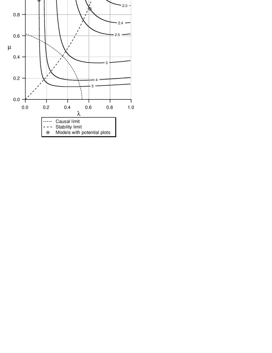
Figure 1: The $\lambda\mu$ parameter space of the GB5 family. The pressure and energy density satisfy the physical requirements $p\geq 0$, $\rho\geq 0$ and ${\rm d}p/{\rm d}\rho\geq 0$. Contours are shown for some values of the tenuity $\alpha=R/M$. Specifying the value of $\lambda$ fixes the equation of state up to a scaling. The corresponding sequence of stellar models can then be followed along the $\lambda=constant$ line starting from the Newtonian limit at $\mu=0$. The mass increases along such a sequence up to the dashed curve after which it decreases. The dashed curve therefore represents the transition to unstable models. The stable region is consequently located to the lower right of the stability limit. The dotted curve is the causal limit. A model is classified as causal if the equation of state satisfies ${\rm d}p/{\rm d}\rho\leq 1$ throughout the interior of the star. For acausal models the speed of sound as defined by $v_{\rm sound}:=\sqrt{{\rm d}p/{\rm d}\rho}$ is therefore larger than the speed of light in some part of the stellar interior. The causal GB5 systems are located at the lower left side of the dotted curve in parameter space. The two marks in the figure are the points which correspond to the models for which potential plots are given in this letter.

One of the two models marked in figure 1 has $\alpha=5$. The scattering potential for that model is shown in figure 2.

Figure 2: The GB5 potential for the model marked on the $\alpha=5$ contour in figure 1 is plotted for $l=2$ along with the exterior potential. For comparison the potential of the uniform density model with the same mass and radius is shown as the dashed curve.

This clearly illustrates the fact that the potential may have a minimum in the stellar interior even though the outer parts of the star extend to regions well beyond $\alpha=3$. We also mention without proof that this model admits a family of closed null geodesics in its interior. It may be objected that the model is unstable (as indicated in figure 1) and that this result therefore has little physical relevance. However, the instability is closely connected with the softness of the equation of state. Taking instead the double layer uniform density models mentioned in the introduction it should be possible to provide examples of stable models having a potential with a minimum in the interior. A second comment we wish to make on this issue is that resonances in unstable models may in principle be important in gravitational collapse situations where short-lived unstable equilibrium states could perhaps form en route to the final collapse.

The second model indicated in figure 1 has $\alpha=2.4$ and lies in the stable region of the parameter space. The corresponding potential is plotted in figure 3.

Figure 3: The potential for the second GB5 model marked in figure 1 is plotted for $l=2$. As in figure 2 the dashed curve is the potential of the corresponding uniform density model.

The phenomenon we wish to illustrate here is that the GB5 potential has a significantly deeper potential well than a uniform density model with the same mass and $R/M$ ratio. The quasi-normal modes of the uniform density model with $\alpha=2.4$ were calculated in [1]. It would be interesting to calculate the modes for the GB5 model. The deeper minimum is an indication of longer damping times compared to the uniform density case.

The question of whether realistic stellar models can be ultracompact (in the sense defined in this letter) remains open. In [7], Iyer, Vishveshwara and Dhurandar searched for stable and causal models satisfying $R<3M$. In view of the results given in the present work it would be more relevant to look for stable and causal models which are ultracompact in the sense of having a family of closed null geodesics in the stellar interior. It would be very useful to have a simple rough criterion of ultracompactness expressed in terms of a dimensionless combination of easily computable quantities. Examples of criteria of compactness include the central redshift (defined as the redshift of a hypothetical speed of light signal sent from the center of the star and received by a static observer at infinity) and the central 4-dimensional curvature, for example $(R^{\alpha\beta\gamma\delta}R_{\alpha\beta\gamma\delta})_{\rm c}$ or $(R^{\alpha\beta}R_{\alpha\beta})_{\rm c}$. The redshift is already dimensionless while the curvature measures need to be properly normalized for example by multiplying by a power of the total mass. However, it is not clear whether any of these measures, either by themselves or by taking combinations, could serve as criteria for ultracompactness.

References

- [1] S. Chandrasekhar and V. Ferrari, Proc. Roy. Soc. Lond. A 434, 449 (1991).
- [2] K. D. Kokkotas, Mon. Not. R. Ast. Soc. 268, 1015 (1994).
- [3] N. Andersson, Y. Kojima, and K. D. Kokkotas, Astrophys. J. 462, 855 (1996).
- [4] Y. Kojima, N. Andersson, and K. D. Kokkotas, Proc. Roy. Soc. Lond. A 434, 341 (1995).
- [5] M. A. Abramowicz et al., Class. Quantum Grav. 14, L189 (1997).
- [6] H. A. Buchdahl, Phys. Rev. 116, 1027 (1959).
- [7] B. R. Iyer, C. V. Vishveshwara, and S. V. Dhurandar, Class. Quantum Grav. 2, 219 (1985).
- [8] L. Lindblom, Phys. Rev. D 58, 024008 (1998).
- [9] W. Simon, Gen. Rel. Grav. 26, 97 (1994).
- [10] K. Rosquist, Class. Quantum Grav. 12, 1305 (1995).
- [11] S. Chandrasekhar and V. Ferrari, Proc. Roy. Soc. Lond. A 432, 247 (1991).
- [12] S. Sonego and M. Massar, Mon. Not. R. Ast. Soc. 281, 659 (1996).