Spherically symmetric static solution for colliding null dust

Abstract

The Einstein equations are completely integrated in the presence of two (incoming and outgoing) streams of null dust, under the assumptions of spherical symmetry and staticity. The solution is also written in double null and in radiation coordinates and it is reinterpreted as an anisotropic fluid. Interior matching with a static fluid and exterior matching with the Vaidya solution along null hypersurfaces is discussed. The connection with two-dimensional dilaton gravity is established.

I Introduction

Null dust represents the high frequency (geometrical optics) approximation to the unidirectional radial flow of unpolarized radiation. This is a reasonable approximation whenever the wavelength of the radiation is negligible compared to the curvature radius of the background. Various exact solutions of the Einstein field equations were found in the presence of pure null dust (for reviews see [1], and more recently [2] and [3]).

In some scenarios even gravitation behaves as null dust. Price [4, 5] has shown that a collapsing spheroid radiates away all of its initial characteristics excepting its mass, angular momentum and charge. (This result is known as the no hair theorem.) The escaping radiation then interacts with the curvature of the background being partially backscattered. Both the escaping and the backscattered radiation can be modeled by null dust [6] as the curvature radius of the background is larger than the wavelength of the radiation.

Letelier has shown that the matter source composed of two null dust clouds can be interpreted as an anisotropic fluid [7], giving also the general solution for plane-symmetric anisotropic fluid with two null dust components. Later Letelier and Wang [8] have discussed the collision of cylindrical null dust clouds. The collision of spherical null dust streams was discussed by Poisson and Israel [6]. Their analysis yielded the phenomenon of mass inflation.

However, no exact solution in the presence of two colliding null dust streams with spherical symmetry was known until now. Recently Date [9] tackled this problem under the assumption of staticity, integrating part of the Einstein equations. It is the purpose of the present paper to present the exact solution for the case of two colliding spherically symmetric null dust streams in equilibrium, in a completely integrated form.

The plan of the paper is as follows. In Sec. II we derive the field equations and we integrate them. The emerging exact solution is written explicitly in suitable coordinates adapted to spherical symmetry and staticity. The metric in radiation coordinates and in double null coordinates is also given. We analyze the metric both analytically and by numeric plots. In Sec. III we present various possible interpretations of the solution, including the anisotropic fluid picture, and dilatonic gravity.

Finally Sec. IV contains the analysis of the interior and exterior matching conditions on junctions along timelike and null hypersurfaces, respectively. We employ the matching procedure of Barrabès and Israel [10]. The interior junction fixes the parameters of the solution in terms of physical characteristics of the central star: the mass and energy density on the junction. The exterior matching with incoming and outgoing Vaidya solutions [11] leads to the conclusion that no distributional matter is present at the junction. This feature is in contrast with the exterior matching with the Schwarzschild solution [9].

II Solution of the Einstein Equations

The general form of a spherically symmetric, static metric in a spacetime with topology $R^{2}\times S^{2}$ is

$$ds^{2}=-h(r)dt^{2}+f(r)^{-1}dr^{2}+r^{2}d\Omega^{2}.$$ (1)

Here $t$ is time, $r$ is the curvature coordinate (e.g. the radius of the sphere $t$=const with area $4\pi r^{2}$), $d\Omega^{2}=d\theta^{2}+\sin^{2}(\theta)d\phi^{2}$ is the square of the solid angle element. The functions $f(r)$ and $h(r)$ are positive valued. We introduce the local mass function $m(r)$, related to the gravitational energy within the sphere of radius $r$ [12]:

$$f(r)=1-\frac{2m(r)}{r}\ .$$ (2)

The energy-momentum tensor in the region of the cross-flowing null dust is a superposition of the energy-momentum tensors of the incoming and outgoing components:

$$T^{ab}=\frac{\beta(r)}{8\pi r^{2}}(v^{a}v^{b}+u^{a}u^{b}).$$ (3)

All energy conditions are satisfied for $\beta(r)\geq 0$. The same linear mass density function $\beta$ was chosen for both components as staticity requires no net flow in either of the null directions. The vector fields

$$v^{a}=\frac{1}{\sqrt{2}}\left(\frac{1}{\sqrt{h}},\sqrt{f},0,0\right),\qquad u^{a}=\frac{1}{\sqrt{2}}\left(\frac{1}{\sqrt{h}},-\sqrt{f},0,0\right)$$ (4)

are the tangents to the (future-oriented) outgoing and incoming null congruences, partially normalized such that $v^{a}u_{a}=-1$. Similarly as for the one-component null dust, here both null congruences are geodesics [9].

After eliminating second time derivatives from the nontrivial Einstein equations we have the system:

$$r\frac{df}{dr} = -\beta-f+1$$ (5)

$$rf\frac{dh}{dr} = h(\beta-f+1)$$ (6)

$$rf\frac{d\beta}{dr} = \beta(-\beta+f-1)\ .$$ (7)

The solutions with $\beta$=const all reduce to $\beta=0$, meaning vacuum. They are either the Schwarzschild or the flat solution, in accordance with the Birkhoff theorem. For $\beta\neq$const one of the equations is a relation between the mass density $\beta(r)$ and the metric function $h\left(r\right)$:

$$h=\frac{A}{\beta},$$ (8)

where $A>0$ is a constant. This relation can be deduced also from the energy-momentum conservation[9]. The remaining equations do not contain the constant $A$:

$$f\frac{d\ln f}{d\ln r} = -\beta-f+1$$ (9)

$$f\frac{d\ln\beta}{d\ln r} = -\beta+f-1\ .$$ (10)

Inserting (2) in (9) the mass is found to increase with the radius: $dm/dr=\beta/2>0$.

Now we solve the system (9),(10). Following Date[9] , we eliminate $f$ from (9) by its expression taken from (10):

$$f=\frac{1+\beta}{1-\frac{d\ln\beta}{d\ln r}}.$$ (11)

The resulting second order ordinary differential equation in $1/\beta$ can be integrated, finding:

$$\frac{d}{d\ln r}\left(\frac{1}{\beta}\right)=\left(D-\frac{1}{\beta}-2\ln\frac{\beta}{r}\right)\frac{1}{1+\beta}.$$ (12)

Here $D$ is an integration constant. Inserting this expression in (11), an algebraic relation between the metric components emerges:

$$\frac{(1+\beta)^{2}}{2f\beta}=\ln\left(\frac{Cr}{\beta}\right),$$ (13)

where $C=\exp((1+D)/2)>0$.

Then we complete the integration of the system (9),(10). The key remark is that none of the equations in this system contains explicitly the independent variable $\ln r$. Thus one can pass to the new independent variable $\beta$, in terms of which an ordinary first order equation can be written:

$$\frac{df}{d\beta}=\frac{f(\beta+f-1)}{\beta(\beta-f+1)}\ .$$ (14)

Introducing the new positive variables

$$P=(2f\beta)^{1/2},\ \qquad L=\frac{1+\beta}{(2f\beta)^{1/2}}$$ (15)

the equation (14) takes the form of a first order linear (inhomogeneous) ordinary differential equation:

$$\frac{dP}{dL}=2\left(1-PL\right)\ .$$ (16)

The solution is found by integrating first the homogeneous equation, then varying the constant. It is

$$P=2e^{-L^{2}}\Phi_{B}(L)\;,\qquad\Phi_{B}(L)=B+\int^{L}e^{x^{2}}dx>0,$$ (17)

where $B$ is a third integration constant. The function $\Phi_{B}(L)$ in (17) can be expressed either in terms of the error function or in terms of the Dawson function:

$$\Phi_{B}(L)-B=-\frac{i\sqrt{\pi}}{2}\mathop{\rm erf}(iL)=e^{L^{2}}Dawson(L).$$ (18)

For properties of these transcendental functions see[13].

From Eqs. (13),(15) and (17) both the curvature coordinate $r$ and the metric functions $\beta$ and $f$ are found as functions of the radial variable $L$:

$$Cr(L) = -e^{L^{2}}+2L\Phi_{B}(L)$$ (19)

$$\beta(L) = -1+2Le^{-L^{2}}\Phi_{B}(L)$$ (20)

$$f(L) = \frac{2\Phi_{B}^{2}(L)}{e^{L^{2}}\left[-e^{L^{2}}+2L\Phi_{B}(L)\right]}.$$ (21)

Then the mass function $m=m\left(L\right)$ is obtained from (2):

$$2Cm(L)=-e^{L^{2}}+2L\Phi_{B}(L)-2e^{-L^{2}}\Phi_{B}^{2}(L).$$ (22)

It is easy to check that both $r$ and $m$ are monotonously increasing functions of $L$:

$$\frac{d\left(Cr\right)}{dL}= 2\Phi_{B}(L)>0$$ (23)

$$\frac{d\left(Cm\right)}{dL}=e^{-L^{2}}\Phi_{B}(L) \left[-e^{L^{2}}+2L\Phi_{B}(L)\right]\geq 0.$$ (24)

In the last relation the equality holds for $r=0$.

Now we have everything together to write the metric in terms of the new radial coordinate $L$:

$$ds^{2}=\frac{-Ae^{L^{2}}dt^{2}}{-e^{L^{2}}+2L\Phi_{B}(L)}+2e^{L^{2}}\left[-e^{L^{2}}+2L\Phi_{B}(L)\right]\frac{dL^{2}}{C^{2}}+\left[-e^{L^{2}}+2L\Phi_{B}(L)\right]^{2}\frac{d\Omega^{2}}{C^{2}}.$$ (25)

There are three parameters in the solution, two of them restricted to be positive: $A$ and $C$. Without loss of generality we can choose $A=1$ by rescaling the time coordinate. The parameter $C$ provides some distance scale. We comment on the third parameter in what follows. Both $Cr\geq 0$ and the energy conditions $\beta\geq 0$ imply

$$B\geq\chi(L)\ ,\quad\chi(L)=\frac{e^{L^{2}}}{2L}-\int^{L}e^{x^{2}}dx$$ (26)

valid for all admissible values of $L$. The equality $B=\chi(L_{0})$ holds for $L=L_{0}$ corresponding to $r=0$. As $d\chi/dL=-e^{L^{2}}/2L^{2}<0$, the function $\chi(L)$ is monotonously decreasing and the inequality (26) will be satisfied for any $L>L_{0}$. Thus $B$ gives the lower boundary $L_{0\text{ }}$for the range of the radial coordinate $L$.

Next we plot numerically the functions $\beta(r)$, $f(r)$ and $m\left(r\right)$ for different values of the parameter $B$ (Figs.1-3).

FIG. 1.: (a) The function $\beta=\beta(\ln r)$ at parameter values $B=C=1$. The metric is singular at $r=0$ and the space-time is not asymptotically flat. (b) Plot of $\beta=\beta(\ln r,B)$ for $C=1$ and $0\leq B\leq 7$.

FIG. 2.: (a) The function $\ln f=\ln f(\ln r)$ at parameter values $B=C=1$. (b) Same for $0\leq B\leq 7$.

FIG. 3.: (a) The mass function $m=m(\ln r)$ at parameter values $B=C=1$ takes negative values close to $r=0$. (b) The mass function in the parameter region $0\leq B\leq 7$. The value of $r$ where the mass becomes negative depends on the parameter $B$.

As we see from Fig. 3, the mass function vanishes at some radius $\tilde{r}$ and takes negative values at $r<\tilde{r}$. We show here that such a positive $\tilde{r}$ exists irrespective of the choice of the parameters $B$ and $C$. By combining (19) and (22) with the condition $m=0$ we find $\tilde{r}=2\Phi_{B}^{2}(\tilde{L})/C\exp(\tilde{L}^{2})>0$. The constant $C$ has a simple scaling effect on the value of $\tilde{r}$. Figure 3(b) shows that in the domain $(0,7)$ the negative mass region can be extended by increasing $B$. We emphasize that the energy conditions are still satisfied in the negative mass regions. The interpretation of the negative mass function is not immediate and depends on the measuring procedure of the mass in this asymptotically non-flat space-time.

At the end of this section we give the metric in double null and radiation coordinates. This requires an additional integration. We introduce a “tortoise coordinate” $r^{*}$ in the same manner it can be introduced in the Schwarzschild space-time:

$$r^{*}=\int^{r}\frac{dr^{\prime}}{\left[f(r^{\prime})h(r^{\prime})\right]^{1/2}}=\frac{\sqrt{2}}{C}\int^{L}\left[-e^{y^{2}}+2y\Phi_{B}(y)\right]dy.$$ (27)

The radial null geodesics are $t=t_{0}+cr^{*}$, with $c=1$ for incoming and $c=-1$ for outgoing geodesics.

Introducing the null coordinates $x^{\pm}=t\pm r^{*}$ the metric takes the simple form:

$$ds^{2}=-h(x^{+},x^{-})dx^{+}dx^{-}+r^{2}(x^{+},x^{-})d\Omega^{2}.$$ (28)

The radial null geodesics are now $x^{\pm}$=const. The functions $h(x^{+},x^{-})=h(x^{+}-x^{-})$ and $r(x^{+},x^{-})=r(x^{+}-x^{-})$ are contained in implicit form in Eqs. (8),(27), (19) and ( 20).

Finally we cast our static, spherically symmetric solution of crossflowing null dust in either the incoming or outgoing radiation coordinates $(v=t+cr^{*},r,\theta,\phi)$. These coordinates are like the Eddington-Finkelstein coordinates for the Schwarzschild solution. If the solution was asymptotically flat, they would be the Bondi-Sachs coordinates.

$$ds^{2}=-\left(f\beta\right)^{-1/2}dv\left[\left(\frac{f}{\beta}\right)^{1/2}dv-2cdr\right]+r^{2}d\Omega^{2}.$$ (29)

Here $v=x^{\pm}$ for $c=\pm 1$. In these coordinates the radial null geodesics are given by one of the equations $v$=const and

$$v=const+2c\int^{r}\left(\frac{\beta\left(r^{\prime}\right)}{f\left(r^{\prime}\right)}\right)^{1/2}dr^{\prime}.$$ (30)

Now it is evident that there is no apparent horizon:

$$\frac{dr}{d\left(cv\right)}=\frac{1}{2}\left(\frac{f}{\beta}\right)^{1/2}>0,$$ (31)

thus no event horizon either. Thus the singularity in the origin $r=0$ is naked. This is very similar to the naked singularity of the negative mass Schwarzschild solution [9].

III Interpretation of the Solution

A 2D dilatonic model

In this subsection we present a dilatonic model which in 4D has the interpretation of a spherically symmetric gravitational field in the presence of two crossflowing null dust streams. This dilatonic model emerges from the action

$$S=\int d^{2}x\sqrt{-g}\rho\left[R\left[g\right]+\frac{1}{2}g^{\alpha\beta}\nabla_{\alpha}\ln\rho\nabla_{\beta}\ln\rho+\frac{2}{\rho}\right]-\frac{1}{2}\int d^{2}x\sqrt{-g}g^{\alpha\beta}\nabla_{\alpha}\varphi\nabla_{\beta}\varphi\ .$$ (32)

The first term is the Einstein-Hilbert action reduced by spherical symmetry (a surface term was dropped). The second term in (32) represents a 2D massless scalar field in minimal coupling. The minus sign assures that all 4D energy conditions are satisfied. $\rho=r^{2}$ is the dilaton and $\varphi$ is the scalar field. The conformal flatness of the $2\times 2$ metric $g_{\alpha\beta}=h\eta_{\alpha\beta}$ is manifest in the corresponding 4D line element (28). $\nabla$ and $R\left[g\right]$ are the covariant derivative and curvature scalar, respectively associated with the metric $g$. Although the equations emerging from this model are quite similar to the corresponding equations in the Callan-Giddings-Harvey-Strominger (CGHS) model[14], they could not be exactly integrated in general. For our purposes we take only the equation emerging from variation of the scalar field, in double null coordinates:

$\displaystyle\varphi,_{+-}=0$

Here commas denote derivatives. The equation has the D’Alembert solution

$$\varphi=\varphi^{+}\left(x^{+}\right)+\varphi^{-}\left(x^{-}\right),$$ (33)

showing that the scalar field behaves like our matter source of crossflowing null dust. The 4D interpretation of the particular solution with either leftmoving or rightmoving matter is the Vaidya solution[11]. Recently Miković has given a solution [15] for the case where both components are present, in the form of a perturbative series in powers of the outgoing energy-momentum component.

Our static solution (28) represents the first explicit exact solution for this model, when none of the null dust components are neglected.

B Anisotropic fluid

Following Letelier [7] we reinterpret the energy-momentum tensor (3) as describing an anisotropic fluid with a pressure component equaling its energy density:

$$T_{ab} = \rho(U_{a}U_{b}+\chi_{a}\chi_{b})$$ (34)

$$-U_{a}U^{a} = \chi_{a}\chi^{a}=1\;,\qquad U_{a}\chi^{a}=0\ .$$ (35)

A straightforward comparison with (3) gives

$$\rho = \frac{\beta}{8\pi r^{2}},\qquad$$ (36)

$$U^{a} = \frac{1}{\sqrt{2}}\left(v^{a}+u^{a}\right)=\frac{1}{\sqrt{h}}\left(\frac{\partial}{\partial t}\right)^{a}$$ (37)

$$\chi^{a} = \frac{1}{\sqrt{2}}\left(v^{a}-u^{a}\right)=\sqrt{f}\left(\frac{\partial}{\partial r}\right)^{a}.$$ (38)

Thus the solution represents an anisotropic fluid at rest with the energy density $\rho$ and radial pressure $p=\rho.$ No tangential pressures in the spheres $r$=const are present. The fluid is isotropic only about a single point, the origin.

C Radiation atmosphere

The solution can be interpreted as the outer region of a radiating star, receiving radiation from the surrounding region either. If equilibrium is achieved between the two components, we have the static solution (25). This was the initial interpretation proposed by Date [9] .

We write the energy-momentum tensor of the static solution in the double null coordinate system $(x^{+},x^{-},\theta,\phi)$. Inserting the null covectors

$$v_{a}=\left(0,-\sqrt{\frac{h}{2}},0,0\right),\qquad u_{a}=\left(-\sqrt{\frac{h}{2}},0,0,0\right)$$ (39)

in the covariant form of (3) and taking account of (8) the energy-momentum tensor becomes

$$T_{ab}dx^{a}dx^{b}=\frac{1}{16\pi r^{2}}\left(dx^{+}dx^{+}+dx^{-}dx^{-}\right),$$ (40)

a superposition of two cross-flowing null dust streams with equal and constant mass density functions. However one can freely rescale the null vectors $v^{a}$ and $u^{a\text{ }}$ to have arbitrary mass density functions either. After such a rescaling the mass density function of the incoming null dust depends only on the outgoing coordinate $x^{+}$ and viceversa, a property pertinent to the mass functions of the Vaidya solution [11], characterized by the energy-momentum tensor

$$T_{ab}dx^{a}dx^{b}=\frac{c}{4\pi r^{2}}\frac{dM(V)}{dV}dVdV.$$ (41)

$M(V)$ is the mass function and the coordinate $V$ is outgoing for incoming radiation and incoming for outgoing radiation.

In the next section we will study the interior junction with a static star, and the exterior junction with incoming and outgoing Vaidya solutions.

IV Junction Conditions

A Matching with interior spherically symmetric static solutions

We discuss the junction with an interior solution with accent on the anisotropic fluid interpretation given previously. A similar treatment was given in [9]. Both our analysis and the one in [9] reveals that the junction with a static interior matter can be done without a regularizing thin shell. Our treatment is more general, however. We formulate the junction conditions for two generic static spherically symmetric space-times, following the standard Darmois-Israel junction procedure [16, 17] and we establish a constraint on the matter pressures implied by the matching conditions. An other improvement over [9] is due to the fact that we dispose of the exact solution (25), thus the explicit computation of the the matching conditions with an arbitrary particular interior becomes possible.

An orthonormal basis is given by the vectors $U$ and $\chi$ defined by Eqs. (37) and (38) together with the spacelike vectors

$$E_{{\bf 3}}=\frac{1}{r}\frac{\partial}{\partial\theta}\;,\qquad E_{{\bf 4}}=\frac{1}{r\sin\theta}\frac{\partial}{\partial\phi}.$$ (42)

Any spherically symmetric static energy-momentum tensor has the form

$$T^{ab}=\rho U^{a}U^{b}+p_{1}\chi^{a}\chi^{b}+p_{2}\left(E_{{\bf 3}}^{a}E_{{\bf 3}}^{b}+E_{{\bf 4}}^{a}E_{{\bf 4}}^{b}\right).$$ (43)

By inserting $p_{i}=\alpha_{i}/8\pi r^{2}$ and $\rho$ in the form (36) in the Einstein equations for the metric (1) we find

$$r\frac{df}{dr} = -\beta-f+1$$ (44)

$$rf\frac{dh}{dr} = h(\alpha_{1}-f+1)$$ (45)

$$2rf\frac{d\alpha_{1}}{dr} = -\alpha_{1}^{2}+\alpha_{1}(-\beta+f-1)+\beta(f-1)+4\alpha_{2}f.$$ (46)

The induced metric of the surface $r$=const is

$$ds_{\Sigma}^{2}=-hdt^{2}+r^{2}d\Omega^{2}\ .$$ (47)

Without loss of generality we can choose the time coordinates in both static space-times such that they are continuous on the junction. Then the continuity of the first fundamental form requires the metric function $h$ to be continuous.

The extrinsic curvature of the junction surface $r=const$ is defined as

$$K_{ab}=\left(\delta_{a}^{c}-\chi^{c}\chi_{a}\right)\left(\delta_{b}^{d}-\chi^{d}\chi_{b}\right)\nabla_{c}\chi_{d}\ .$$ (48)

The nonvanishing components are:

$$K_{tt}=\frac{h}{2r\sqrt{f}}(-\alpha_{1}+f-1)\;,\qquad K_{\theta}^{\theta}=K_{\phi}^{\phi}=\frac{\sqrt{f}}{r}\ .$$ (49)

In the above expressions the derivatives were eliminated by use of Eq. (45).

Continuity of the extrinsic curvature across the junction hypersurface $r=r_{1}$ is achieved, provided that the metric and the function $\alpha_{1}$ (thus also $p_{1}$) are continuous. We have proved the following result:

Any two spherically symmetric static solutions can be matched along hypersurfaces $r=const$ provided the radial pressures are continuous. This is similar to the theorem given by Fayos, Jaén, Llanta and Senovilla [18] for the matching of the Vaidya solution with a generic spherically symmetric solution along timelike hypersurfaces. A generic discussion on matching spherically symmetric space-times along thin spherical timelike shells can be found in[19].

For the double null dust solution $\alpha_{1}=\beta$. In consequence the interior fluid should have a radial pressure equal to the energy density (36) of the double null dust solution on the junction. However, no conditions on the pressures tangent to the spheres emerge.

We see from Eqs. (20), (22) and (36) that the integration constants $B$ and $C$ appear in the radial pressure and mass function of the static double null dust solution. Continuity of these functions on the junction fixes the value of the constants, once the interior solution is chosen. For a realistic star, the mass $M_{1}$ should be positive. This implies a lower boundary for the possible values of $r_{1}$, as follows from Fig. 3(a).

Let us illustrate the junction with the interior Schwarzschild solution[20] $ds^{2}=-\left(a-b\sqrt{1-r^{2}/R^{2}}\right)^{2}dt^{2}+\left(1-r^{2}/R^{2}\right)^{-1}dr^{2}+r^{2}d\Omega^{2}$, with the energy density $\rho_{S}=3/R^{2}$=const and pressure $p_{S}$ given by

$$8\pi p_{S}=\frac{3b\sqrt{1-\frac{r^{2}}{R^{2}}}-a}{R^{2}\left(a-b\sqrt{1-\frac{r^{2}}{R^{2}}}\right)}\ .$$ (50)

Several relations among the Schwarzschild parameters $a,b,R$, radius of the star $r_{1}$ and the parameters $B$ and $C$ emerge from the junction conditions:

$$2m_{1}=\frac{r_{1}^{3}}{R^{2}}\ ,\qquad 2a=\frac{3}{\sqrt{\beta_{1}}}+\frac{R^{2}}{r_{1}^{2}}\sqrt{\beta_{1}}\ ,\qquad 2b\sqrt{1-\frac{r_{1}^{2}}{R^{2}}}=\frac{1}{\sqrt{\beta_{1}}}+\frac{R^{2}}{r_{1}^{2}}\sqrt{\beta_{1}}\ .$$ (51)

We have denoted by $\beta_{1}$ and $m_{1}$ the values of the functions $\beta$ and $m$ at the junction $r=r_{1}$. The first two relations (51) determine the constant $B$ and the value of the radial coordinate $L_{1}$ at the junction in terms of $r_{1}/R$ and $a$, when Eqs. (19), (20) and (22) are inserted. Eliminating $\beta_{1}$ from the last two relations of (51), a constraint $b=b(a,r_{1}/R)$ on the possible values of characteristics of the interior emerges. Finally (19) implies $C=C(a,r_{1}/R,r_{1})$.

In the light of the above relations we see that after choosing some value for $C$ (a scale), the constant $B$ is determined exclusively by the radius and density (or mass) of the star.

B Matching with Vaidya solutions

In this subsection we study the junctions with the incoming and outgoing Vaidya solutions, which are at the exterior of the static double null dust solution. There are only three points (in fact spheres) in common with exterior Schwarzschild regions (Fig. 4), and the matching can be done without introducing regularizing thin shells.

The high-frequency approximation to the unidirectional radial flow of spherically symmetric unpolarized radiation, characterized by the energy-momentum tensor (41) is represented by the Vaidya solution[11]:

$$ds^{2}=-dV\left[\left(1-\frac{2M(V)}{r}\right)dV-2cdr\right]+r^{2}d\Omega^{2}.$$ (52)

The radial null geodesics are the lines $V$=const and the curves given by

$$\frac{dr}{dV}=\frac{c}{2}\left(1-\frac{2M(V)}{r}\right).$$ (53)

We would like to match our static solution with incoming and outgoing Vaidya solutions along the outgoing, respectively incoming radial null geodesics, e.g. along lines of constant incoming, respectively outgoing coordinate (Fig 4.). These are given by Eq. (53) in the Vaidya solution and by Eq. (30) in the static solution.

A convenient formalism for matching solutions along null surfaces, which does not require coordinates that match continuously on the shell, was developed by Barrabès and Israel[10]. Their discussion on the particular case of spherical symmetry requires the metric in both space-times written in the form:

$$ds^{2}=-e^{\psi}dz\left[fe^{\psi}dz-2dr\right]+r^{2}d\Omega^{2}.$$ (54)

Here $f$ and $\psi$ depend on both $r$ and $z$. The null coordinate $z$ is always outgoing but it can be either increasing or decreasing with time. Then the junction is done along the null hypersurfaces $z$=const.

To apply this formalism it would be desirable to express the Vaidya solution in the other set of radiation coordinates $[U(V,r),r,\theta,\phi]$ in which Eq. (53) takes the form $U$=const. However, this is possible only when double null coordinates are found. It was demonstrated in [21] that double null coordinates exist when the mass is a linear or exponential function of the advanced or retarded time $V$. We argue in what follows that the mass function of that particular Vaidya solution, which is matching continuously to the static solution has a more complicated dependence. A further inconvenience is that there is no obvious choice for the intrinsic coordinates in terms of the space-time coordinates in the null junction hypersurface. For these reasons we proceed as follows. First we find coordinates that match continuously on the junction and in terms of which the metric is continuous. Then we employ the Barrabès-Israel junction formalism to find the distributional stress-energy tensor on the junction.

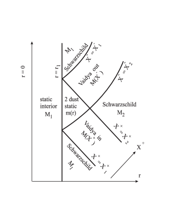
FIG. 4.: The intersection of two crossflowing null dust streams with mass functions $M(V)$ is the static solution characterized by the mass function $m(r)$. Here $V=X^{\pm}$ stands for $c=\pm 1$ and $X^{\pm}$ are the advanced (retarded) time in the Vaidya solution. The 2-dust solution touches in three points exterior Schwarzschild regions with masses $M_{1}$ and $M_{2}$. At the interior junction there is a static fluid representing a star with mass $M_{1}$ . The mass functions $M(V)$ of the Vaidya regions change monotonously from $M_{1}$ to $M_{2}$ .

As a radial variable of both metrics we choose $L$ by extending the expression (19) of $r=r(L)$ to the Vaidya regions too. An appropriate null coordinate $z$ is defined by the values of $L=L_{j}$ on the junction. In these coordinates the junction hypersurfaces are characterized by the null geodesic equations $z=L$ in both space-times. We proceed in deriving the expressions of the coordinates $v$ and $V$ and of the mass function $M$ in terms of the coordinate $z$.

Identifying the corresponding part of Eq. (40) with Eq. (41 ), we find the relation between the null coordinates $V$ and $v$, valid on the junction :

$$dv=2\left(c\frac{dM(V)}{dV}\right)^{1/2}dV.$$ (55)

Then we extend this relation over both the static and the Vaidya regions.

The null geodesic equation (30) of the static solution, evaluated on the junction (where $z=L$) gives

$$\frac{dz}{dV}=\frac{c}{2r^{2}}\frac{dM}{dz}$$ (56)

Inserting Eq. (56) in the null geodesic equation (53) of the Vaidya solution we find its mass function in terms of the new null coordinate $z$:

$$2CM(z)=-e^{z^{2}}+2z\Phi_{B}(z)-2e^{-z^{2}}\Phi_{B}^{2}(z).$$ (57)

Thus the mass function is continuous at the junction. The geodesic equation (56) together with (57) gives the relation between the null coordinates $V$ and $z$:

$$V\left(z\right)=const+\frac{2c}{C}\int^{z}\frac{e^{y^{2}}\left[-e^{y^{2}}+2y\Phi_{B}(y)\right]dy}{\Phi_{B}(y)}.$$ (58)

The relations (57) and (58) contain in implicit form the dependence of the mass function $M$ of the Vaidya solution on the radiation coordinate $V$. Despite the complicated dependence $M(V)$ it is straightforward to check that $M$ satisfies the required monotonicity condition:

$$2\frac{dM}{d(cV)}=\frac{\Phi_{B}^{2}(z)}{e^{2z^{2}}}>0\ .$$ (59)

Finally Eqs. (55) and (58) give $v=v\left(z\right)$:

$$v\left(z\right)=const+\frac{2\sqrt{2}c}{C}\int^{z}\left[-e^{y^{2}}+2y\Phi_{B}(y)\right]dy.$$ (60)

Now we express both metrics in terms of the coordinates $(z,r(L),\theta,\phi)$. They take the form (54) with

$$f = 1-\frac{2m\left(L\right)}{r\left(L\right)}\;,\qquad e^{\psi}=\frac{2}{C}\frac{e^{L^{2}}}{\Phi_{B}(L)}\left[-e^{z^{2}}+2z\Phi_{B}(z)\right]$$ (61)

$$f_{V} = 1-\frac{2M\left(z\right)}{r\left(L\right)}\;,\qquad e^{\psi_{V}}=\frac{2}{C}\frac{e^{z^{2}}}{\Phi_{B}(z)}\left[-e^{z^{2}}+2z\Phi_{B}(z)\right].$$ (62)

Here the index $V$ refers to the Vaidya solution and the expressions $r\left(L\right),m\left(L\right)$ and $M\left(z\right)$ are given by Eqs. (19), (22) and (57), respectively. We have completed the task of writing both metrics in coordinates which are continuous on the junction and in terms of which the metric is continuous.

It is immediate to check the continuity of the induced metric given by $ds^{2}_{\Sigma}=r^{2}d\Omega^{2}$. The other junction condition is a somewhat subtle issue as the conventional extrinsic curvature tensor for null hypersurfaces carries no transversal information.

We define a pseudo-orthonormal basis [22] $(n,N,E_{{\bf 3}},E_{{\bf 4}})$, where $E_{{\bf 3}}$ and $E_{{\bf 4}}$ are given in Eq. (42) and

$$n=e^{-\psi}\frac{\partial}{\partial z}+\frac{f}{2}\frac{\partial}{\partial r}\;,\qquad N=-\frac{\partial}{\partial r}\;.$$ (63)

The vector $n^{a}$ is orthogonal (and also tangent) to the hypersurfaces $fe^{\psi}dz-2dr=0$, along which the two space-times are glued together. The vector $N^{a}$ is the other radial null vector, transversal to these surfaces. They are related to the previously introduced vectors $v^{a}$ and $u^{a}$ as follows. For the junction with the incoming Vaidya region $v^{a}=\left(2/f\right)^{1/2}n^{a}$ and $u^{a}=\left(f/2\right)^{1/2}N^{a},$ while for the junction with the outgoing Vaidya region $u^{a}=-\left(2/f\right)^{1/2}n^{a}$ and $v^{a}=-\left(f/2\right)^{1/2}N^{a}$.

The projector to these null hypersurfaces with tangent space spanned by $E_{{\bf 3}},E_{{\bf 4}}$ and $n$ is

$$P_{b}^{a}=E_{{\bf 3}}^{a}E_{b}^{{\bf 3}}+E_{{\bf 4}}^{a}E_{b}^{{\bf 4}}-n^{a}N_{b}=\delta_{b}^{a}+N^{a}n_{b}\ .$$ (64)

Following [10] we define the transverse or oblique extrinsic curvature tensor with the aid of the transverse vector $N$:

$$K_{ab}=P_{a}^{c}P_{b}^{d}\nabla_{c}N_{d}\ .$$ (65)

The only nonvanishing components of the transverse extrinsic curvature tensor are

$$K_{zz}=\frac{1}{2}e^{\psi}\partial_{r}\left(fe^{\psi}\right)=\frac{C}{2}e^{\psi}\frac{dL}{d\left(Cr\right)}\partial_{L}\left(fe^{\psi}\right)\;,\qquad K_{\theta}^{\theta}=K_{\phi}^{\phi}=-\frac{1}{r}.$$ (66)

Thus when matching any two metrics of the form (54) on the null hypersurfaces $fe^{\psi}dz-2dr=0$, the jump in the extrinsic curvature is given by the jump in $\partial_{r}\left(fe^{\psi}\right)$, provided the metric is continuous across the junction.

A straightforward computation employing (61) and (62) gives on the junction hypersurfaces of the static double null dust region with the Vaidya regions

$$\partial_{L}\left(fe^{\psi}\right)=\partial_{L}\left(f_{V}e^{\psi_{V}}\right)=\frac{4e^{L_{j}^{2}}\left[-e^{L_{j}^{2}}+2L_{j}\Phi_{B}(L_{j})-e^{-L_{j}^{2}}\Phi_{B}^{2}(L_{j})\right]}{C\left[-e^{L_{j}^{2}}+2L_{j}\Phi_{B}(L_{j})\right]}\ .$$ (67)

In conclusion the extrinsic curvature is also continuous on the junction. There is no need for a thin regularizing shell separating the two domains of the space-time, in contrast to the exterior junction proposed in [9].

V Concluding Remarks

We have integrated the Einstein equations in the presence of crossflowing null dust under the assumptions of spherical symmetry and staticity and analyzed various aspects related to the properties of the emerging exact solution (25). The solution has dilatonic gravity connections and it can be reinterpreted as an anisotropic fluid with radial pressure equal to its energy density and no pressures along the spheres $r$=const. This can be a radiation atmosphere for a star with its radial pressure equal to the energy density of the athmosphere on its surface. No constraint on the pressures along the spherical junction surface was found. On the exterior, the study of the matching conditions with the Vaidya solution revealed no thin shells on the junction.

As a byproduct, we have derived general conditions for the junction of two spherically symmetric solutions. Matching of two static space-times (1) along $r$=const hypersurfaces is assured by the continuity of the metric functions and of the radial pressure. Matching of generic spherically symmetric space-times (54) along the null hypersurfaces $fe^{\psi}dz-2dr=0$ is possible whenever the metric and $\partial_{r}\left(fe^{\psi}\right)$ are continuous.

The negativity of the mass function in some neighbourhood of the $r=0$ singularity raises the possibility of matching this solution to a negative mass core. This may be difficult due to the nontrivial topology of the known negative mass black hole solutions[23]. Despite the lack of experimental evidence for negative mass objects, presumably of quantum origin[9], their microlensing effect[24] on radiation from Active Galactic Nuclei was shown to produce features similar to some observed Gamma Ray Bursts[25].

Equally interesting would be to introduce dynamics in the picture by an interior matching with a collapsing star. We defer this topic to a forthcoming study.

An intriguing open question remains whether exact solutions describing the collision of spherically symmetric null dust streams, which have not reached equilibrium, can be found.

Note added. After the submission of this paper a relevant work in the subject was published by Kramer [26]. The solution presented there is the particular case of the metric (25) with the parameter values $B=0$ and $C=\sqrt{e}$. Our metric functions $h$ and $f$, radial variable $L$ and transcendental function $-e^{L^{2}}+2L\Phi_{B}$ correspond to $e^{2\nu},\ e^{-2\lambda},\ \sqrt{1+2\xi}$ and $\sqrt{e(1+2\xi)}J$, respectively of this paper, when the parameters values $B=0$ and $C=\sqrt{e}$ are chosen. Keeping the parameters arbitrary enabled us in Sec. IV A to match the solution (25) with an interior Schwarzschild solution with arbitrary mass and radius. In contrast with our analysis relying on the Barrabès-Israel matching procedure, in [26] the junction with the Vaidya space-time was discussed by imposing the continuity of the four-metric on the junction.

VI Acknowledgments

The author is grateful to Jiří Bičák, Gyula Fodor, Karel Kuchař and Zoltán Perjés for discussions on the subject and helpful references. This work has been supported by OTKA no. W015087 and D23744 grants. The algebraic packages REDUCE and MAPLEV were used for checking computations and numerical plots.

REFERENCES

- [1] D. Kramer, H. Stephani, M.A.H. MacCallum, and E. Herlt, Exact Solutions of Einstein’s Field Equations (Cambridge University Press, Cambridge, England, 1980).
- [2] D. Kramer, in Rotating Objects and Relativistic Physics, Proceedings, El Escorial, Spain 1992 , edited by J.J.Chinea and L.M. González-Romero (Springer Verlag, Berlin, 1993).
- [3] J. Bičák and K. Kuchař, Phys. Rev. D56, 4878 (1997).
- [4] R. H. Price, Phys. Rev. D5, 2419(1972).
- [5] R. H. Price, Phys. Rev. D5, 2439(1972).
- [6] E. Poisson and W. Israel, Phys. Rev. D41, 1796 (1990).
- [7] P.S. Letelier, Phys. Rev. D22, 807 (1980).
- [8] P.S. Letelier and A. Wang, Phys. Rev. D49, 5105 (1994).
- [9] G. Date, Gen. Relativ. Gravit.29, 953 (1997). Our notation corresponds to of this paper. The scale factor does not appear in our equations and we have chosen the signature of the metric .
- [10] C. Barrabès and W. Israel, Phys. Rev. D43, 1129 (1991). Our notation corresponds to of this paper and we use latin letters for space-time indices.
- [11] P.C. Vaidya, Proc.-Indian Acad. Sci., Sect. A 33, 264 (1951).
- [12] J.L. Synge, Relativity: The General Theory (North-Holland, Amsterdam, 1971), Chap. VII.
- [13] Higher Transcendental Functions (Bateman Manuscript Project) edited by A. Erdélyi et al. (McGraw-Hill, New York, 1953), Vol.2.
- [14] C.G. Callan, S.B. Giddings, J.A. Harvey, and A. Strominger, Phys. Rev. D45, R1005 (1992).
- [15] A. Miković, Phys. Rev. D56, 6067 (1997).
- [16] G. Darmois, in Mémorial des Sciences Mathématiques (Gauthier-Villars, Paris, 1927), Fascicule 25, Chap. V.
- [17] W. Israel, Nuovo Cimento B XLIV, 4349 (1966).
- [18] F. Fayos, X. Jaén, E. Llanta, and J.M.M Senovilla, Phys. Rev. D45, 2732 (1992).
- [19] K. Lake, Phys. Rev. D19, 2847 (1979).
- [20] K. Schwarzschild, Sitz. Preuss. Akad. Wiss., 424 (1916).
- [21] B. Waugh and K. Lake, Phys. Rev. D34, 2978 (1986).
- [22] S.W. Hawking and G.F.R. Ellis, The Large Scale Structure of Space-Time (Cambridge University Press, Cambridge, England, 1973), Chap.4.
- [23] R. Mann, Class. Quantum Grav. 14, 2927 (1997).
- [24] J.G. Cramer, R.L. Forward, M.S. Morris, M. Visser, G. Benford, and G.A. Landis, Phys. Rev. D51, 3117 (1995).
- [25] D.F. Torres, G.E. Romero, and L.A. Anchordoqui, Mod. Phys. Lett. A 13, 1575 (1998).
- [26] D. Kramer, Class. Quantum Grav. 15, L31 (1998).