Causal differencing of flux-conservative equations applied to black hole spacetimes

Abstract

We give a general scheme for finite-differencing partial differential equations in flux-conservative form to second order, with a stencil that can be arbitrarily tilted with respect to the numerical grid, parameterized by a “tilt” vector field $\gamma^{A}$. This can be used to center the numerical stencil on the physical light cone, by setting $\gamma^{A}=\beta^{A}$, where $\beta^{A}$ is the usual shift vector in the 3+1 split of spacetime, but other choices of the tilt may also be useful. We apply this “causal differencing” algorithm to the Bona-Massó equations, a hyperbolic and flux-conservative form of the Einstein equations, and demonstrate long term stable causally correct evolutions of single black hole systems in spherical symmetry.

I Introduction

The apparent horizon boundary condition (AHBC) appears to be one of the fundamental techniques required for evolving black hole spacetimes using numerical techniques. In this paper, we present work on an AHBC in the context of the recently formulated Bona-Massó (BM) hyperbolic system for the Einstein Evolution equations, however in doing so, we present a technique which is generally causally correct for any first order flux-conservative set of PDEs.

The idea of the AHBC was credited to Unruh by Thornburg[1]. The fundamental idea is that, rather than avoiding a singularity by taking slices which delay the infall of observers inside the horizon (eventually requiring an infinite force), one could take regular slices everywhere outside the horizon and place some stable boundary condition inside the apparent horizon, excising a portion of the numerical grid. Mathematically this is consistent because the apparent horizon is known to be inside the event horizon, and the interior of the event horizon is, by definition, causally disconnected from its exterior.

The AHBC in numerical relativity was first shown to work by Seidel and Suen in Ref. [2]. The AHBC proposal by Seidel and Suen has two components. The first is to choose a shift condition which, after some evolution, locks the coordinates by freezing the position of the horizon and keeping radial distances between points constant. In spherical symmetry, this uniquely determines the shift everywhere. Additionally, to handle large shift terms, Seidel and Suen propose re-writing the finite difference representation of the ADM equations to obey the causal structure of the spacetime.

This causal differencing is an important aspect of much AHBC work to date and is generally credited to Seidel and Suen (“causal differencing”) or Alcubierre and Schutz (“causal reconnection”) [3]. The idea proposed by Seidel and Suen is as follows. In the presence of a shift, the Einstein equations have additional terms in the evolution equations (due to the action of ${\cal L}_{\beta}$ on $\gamma_{ij}$ and $K_{ij}$). However, there is another coordinate system in which the shift is zero. Finding the coordinate system, in general, involves integrating a transformation function in time. The Seidel and Suen prescription is to finite difference in the transformed zero shift co-ordinates and then re-transform the finite difference representation to coordinates with a shift.

Using these two techniques, Seidel and Suen proceed to demonstrate that they can accurately evolve Schwarzschild black holes and Schwarzschild black holes with infalling scalar fields for long periods of time.

The followup to Seidel and Suen, a paper by Anninos, Daues, Massó, Seidel and Suen, [4] gave details of the Seidel and Suen causal differencing scheme and presented several shift choices. These shifts allow for coordinate regularity in the entire spacetime and provide horizon locking. Moreover, several of these shifts are extensible to full three dimensional cases, most notably the minimal distortion shift [5]. Using causal differencing and horizon locking shift conditions, Anninos et al. are able to evolve Schwarzschild black holes in spherical symmetry for 1000M with very small errors in the measure of the mass of the horizon, compared to 100% mass errors present in simulations without an AHBC around $t=100M$.

The first application of an AHBC to a hyperbolic scheme was that of Scheel et al. [6]. This scheme used a hyperbolic formulation due to York on a Schwarzschild black hole. The essence of the causal difference scheme was to decompose the time derivative into time evolution along the normal direction and spatial transport due to the shift. That is, they would evolve along the normal direction to some point no longer on their numerical grid, and then re-construct their numerical grid by interpolation. The Scheel et al. approach is roughly equivalent to our advective (non flux-conservative) causal differencer with interpolation after the step, as discussed below. The results of Scheel et al. were initially disappointing, as an instability arose on a short ($10-100M$) time scale. Very recent work [7] has removed this instability by adding constraints to the evolution equations (in a manner specific to spherical symmetry), and run times exceeding $10000M$ have been achieved.

Anninos et al. extended their methods by importing a one dimensional shift into a three dimensional code in [8]. They found a stable horizon mass for a moderate time evolution. This work was extended in the thesis of Greg Daues [9], who applied various shift and excision conditions to three dimensional systems evolved in the ADM formulation, successfully evolving a Schwarzschild hole for 100M using live gauge conditions in three dimensions.

Another demonstration that some aspects of an AHBC could work in three-dimensional numerical relativity was given by Brügmann[10]. Brügmann does not use a shift to freeze the horizon, and only demonstrates his method in geodesically sliced spacetimes. That is, the horizon keeps swallowing grid points as the simulation continues. Nonetheless, he uses an irregular inner boundary on a (semi-adaptive) Cartesian grid and demonstrates a stable evolution for several times longer than the $\pi M$ infall time of the throat in a geodesically sliced spacetime. The inner boundary is simply a few zones inside the location of the (moving) surface $r=2M$, rather than a numerically located horizon. The inner boundary is generated by polynomial extrapolation.

Recently, the Binary Black Hole Grand Challenge has presented several convincing results using an apparent horizon boundary condition with an ADM system using a causal differencing scheme similar to that of Scheel et al. extended to three dimensions. Using boosted Kerr-Schild slices of Schwarzschild with exact gauge conditions, the Grand Challenge was able to transport a black hole across a grid [11]. The Grand Challenge also reports the ability to hold a static black hole static for close to $100M$ in Eddington-Finkelstein slicings in three dimensions.

The work presented below is an attempt to apply similar techniques to those used by Daues and by the Grand Challenge to the BM evolution system, while attempting to exploit the first-order, flux-conservative form of the BM evolution equations. In the first half of the paper, we lay a groundwork for future extensions of the BM system to general three-dimensional BH spacetimes, which are far beyond the scope of this paper, by discussing and analyzing various fully three-dimensional techniques for implementing a general AHBC. In the second half, we apply the general framework to the BM system applied to spherically symmetric vacuum spacetimes, that is, to the Schwarzschild black hole. We evolve initial data taken from three different time-independent slicings of Schwarzschild, all of which are regular at the horizon. We use a lapse and shift imported from the exact solution on all of them, and an exact shift together with a live harmonic slicing condition on one of them. In each of these situations we test one traditional and four causal finite differencing schemes.

II Causal differencing of flux-conservative equations

In this section, we develop causal differencing for an arbitrary system of flux-conservative equations. The equation we want to finite difference is

$${\partial u\over\partial t}+{\partial F^{A}(u)\over\partial x^{A}}=S(u),$$ (1)

where $x^{A}$ are the spatial coordinates, and $u$ is a vector of unknowns. A necessary condition for a stable finite differencing scheme is that all the characteristics of the system lie inside the numerical domain of dependence (“the stencil”). Depending on the formulation of the Einstein equations, there may be mathematical characteristics other than, and in fact outside, the physical light cone. In this paper, we consider only situations where the mathematical characteristics lie inside the physical light cone. In Fig. 1 we show the relationship between the numerical and physical light cone, and show situations in which stable or unstable situations result including a causal differencing case, where we adjust the numerical stencil to follow the physical light cone. The characteristics are not immediately apparent from the form (1) of the equation, but if we are dealing with a hyperbolic formulation of the Einstein equations, perhaps coupled to matter, we know that the (physical) characteristics are centered on the center of the light cones of the spacetime metric

$$ds^{2}=-\alpha^{2}\,dt^{2}+g_{AB}(dx^{A}+\beta^{A}dt)(dx^{B}+\beta^{B}dt).$$ (2)

We now introduce an auxiliary coordinate system $(\tilde{t},\tilde{x}^{a})$ that is related to $(t,x^{A})$ by

$$\tilde{t}=t,\qquad\tilde{x}^{a}=\tilde{x}^{a}(t,x^{A}),$$ (3)

where $\tilde{x}^{a}(t,x^{A})$ obeys the differential equation

$${\partial\tilde{x}^{a}\over\partial t}=\gamma^{A}{\partial\tilde{x}^{a}\over\partial x^{A}}.$$ (4)

The vector field $\gamma^{A}$ distorts the $\tilde{x}$ coordinate system relative to the $x$ coordinate system. We define the shorthands

$$m^{a}\equiv{\partial\tilde{x}^{a}\over\partial t},\qquad{M^{a}}_{A}\equiv{\partial\tilde{x}^{a}\over\partial x^{A}},\qquad{Q^{A}}_{a}\equiv{\partial x^{A}\over\partial\tilde{x}^{a}}.$$ (5)

Note that because $\tilde{t}=t$, $Q$ is also the matrix inverse of $M$.

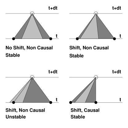
FIG. 1.: We show the stability criterion for light cones and numerical stencils. The light gray areas show the physical past light cone of a given point, and the dark gray areas show the numerical stencil. In the top two figures, where the physical light cone is inside the numerical light cone, we will get a stable evolution. In the non-causal large shift picture, the evolution will not be stable, but tilting the numerical light cone (or causal differencing) will result in a stable evolution.

Assuming for a moment that we choose $\gamma^{A}=\beta^{A}$, the spacetime metric in the new coordinate system is

$$ds^{2}=-\tilde{\alpha}^{2}d\tilde{t}^{2}+\tilde{g}_{ab}d\tilde{x}^{a}d\tilde{x}^{b}.$$ (6)

This has no shift, and therefore the light cone is symmetric around $\partial/\partial\tilde{t}$. The 3-metric, lapse and shift in the two coordinate systems are related by

$$g_{AB}={M^{a}}_{A}{M^{b}}_{B}\,\tilde{g}_{ab},\qquad\alpha=\tilde{\alpha},\qquad\beta^{A}={Q^{A}}_{a}m^{a}.$$ (7)

Our motivation for introducing the auxiliary $\tilde{x}$ coordinates is causal differencing. Here we take causal differencing to mean using a stencil that is symmetrically centered on the light cone. This is equivalent to its being centered on the vector field $\partial/\partial\tilde{t}$ in the new coordinate system. We obtain a “tilted” stencil in the $x$ coordinates by first transforming the differential equation to the $\tilde{x}$ coordinates, using a finite differencing scheme to advance in $\tilde{x}$ coordinates, and transforming the result back to the $x$ coordinates. Although $\gamma^{A}=\beta^{A}$ is the choice that motivates our scheme, we should keep in mind the point of view that $\gamma^{A}$ simply parameterizes a family of tilted stencils for the differential equation (1). No reference needs to be made to either the spacetime metric or the fact that (1) is the Einstein equations. In this respect our scheme differs from the causal differencing schemes suggested by Seidel and Suen [2] and Scheel et al. [6], which explicitly use the fact that the Einstein equations simplify in the $\tilde{x}$ coordinates. In the following sections we consider again a generic tilt vector field $\gamma^{A}$.

A Transforming the differential equation

The partial derivatives in the two coordinate systems are related by

$${\partial\over\partial t} = {\partial\over\partial\tilde{t}}+m^{a}{\partial\over\partial\tilde{x}^{a}},\qquad{\partial\over\partial x^{A}}={M^{a}}_{A}{\partial\over\partial\tilde{x}^{a}},$$ (8)

$${\partial\over\partial\tilde{t}} = {\partial\over\partial t}-\gamma^{A}{\partial\over\partial x^{A}},\qquad{\partial\over\partial\tilde{x}^{a}}={Q^{A}}_{a}{\partial\over\partial x^{A}}.$$ (9)

Transforming (1) to $(\tilde{t},\tilde{x}^{a})$ we obtain

$$\frac{\partial u}{\partial\tilde{t}}+m^{a}\frac{\partial u}{\partial\tilde{x}^{a}}+{M^{a}}_{A}\frac{\partial F^{A}}{\partial\tilde{x}^{a}}=S(u).$$ (10)

We note that this equation is not in flux-conservative form. We will refer to (10) as the advective or non flux-conservative form of our evolution equation. We can put (10) in flux-conservative form by moving $m^{a}$ and ${M^{a}}_{A}$ into the fluxes, giving additional source terms. Doing this, we obtain

$${\partial u\over\partial\tilde{t}}+{\partial\over\partial\tilde{x}^{a}}\left(m^{a}u+{M^{a}}_{A}F^{A}\right)=S(u)+\lambda\,u+\Lambda_{A}F^{A},$$ (11)

where the flux correction coefficients $m^{a}$ and ${M^{a}}_{A}$ have already been defined, and the source correction terms are

$$\Lambda_{A} \equiv {\partial\over\partial\tilde{x}^{a}}{M^{a}}_{A}={\partial\over\partial x^{A}}\ln\det M,$$ (12)

$$\lambda \equiv {\partial\over\partial\tilde{x}^{a}}m^{a}={\partial\over\partial t}\ln\det M.$$ (13)

The second equalities have been written down to clarify the function of the source correction terms, namely to account for a change in the volume element $\det M$. It is useful to note the identity

$$\lambda={\partial\gamma^{A}\over\partial x^{A}}+\gamma^{A}\Lambda_{A}.$$ (14)

We emphasize that when applied to the Einstein Equations, $S(u)$ and $F^{A}$ are the BM sources and fluxes including the shift terms. Even in the case of $\gamma^{A}=\beta^{A}$, we do not cancel these terms from the sources and fluxes, but allow the cancellation to take place numerically (both in the advective and flux-conservative schemes). Below we will explore only the $\gamma^{A}=\beta^{A}$ case numerically, but will find interesting theoretical advantages in the $\gamma^{A}=\tau\beta^{A}$ case (where $\tau$ is some constant).

The advective form of the equation, (10), has several potential numerical advantages over the flux-conservative form, (11). Most notably, the equation $\partial_{t}u=0$ for $u={\mathrm{c}onstant}$ requires cancellations between flux derivatives of the shift and divergences of the shift in the sources in (11), while no such cancellations are needed in (10).

We make the two coordinate systems agree at $t=\tilde{t}=0$:

$$\tilde{x}^{a}(x^{A},0)={\delta^{a}}_{A}x^{A}.$$ (15)

In the remainder of this work we also assume that the tilt is “frozen” in the $x$ coordinates:

$${\partial\over\partial t}\gamma^{A}=0.$$ (16)

In practice, the tilt will be constant only throughout one time step, as described in section II C. For convergence tests, we shall choose it to be constant throughout one time step on the coarsest grid, and accordingly several time steps on the finer grids. After each time step we discard the coordinate system $(\tilde{t},\tilde{x}^{a})$ and start again from scratch. We identify the two coordinate systems either at the end or at the beginning of the time step. The implication of this choice on boundary conditions will be discussed below. We will label the time when the grids coincide as $t=0$, so time steps will go from $t=-\Delta t$ to $t=0$ or from $t=0$ to $t=\Delta t$.

B Calculating the source and flux correction terms

We need to know either the $x^{A}$ traced back to $t=-\Delta t$ along lines of constant $\tilde{x}$ or $\tilde{x}^{a}$ traced forwards along lines of constant $x^{A}$, in order to interpolate the data at the beginning of the time step onto the $\tilde{x}$ grid or reconstruct the $x$ grid after the time step. Rather than by solving the differential equation (4) by finite differencing, we do this by a Taylor series expansion in $t$:

$$x^{A}(\tilde{x},t) = {\delta^{A}}_{a}\tilde{x}^{a}-\gamma^{A}\,t+{1\over 2}\gamma^{B}\gamma^{A}_{,B}\,t^{2}+O(t^{3}),$$ (17)

$$\tilde{x}^{a}(x,t) = {\delta^{a}}_{A}\left[x^{A}+\gamma^{A}\,t+{1\over 2}\gamma^{B}\gamma^{A}_{,B}\,t^{2}+O(t^{3})\right].$$ (18)

In order to calculate the corrected fluxes and sources in the differenced version of (11), we also need to know $m^{a}$, ${M^{a}}_{A}$, $\lambda$ and $\Lambda_{A}$ on the $\tilde{x}^{a}$ grid, at some of the times $t=\pm\Delta t$, $t=\pm\Delta t/2$ and $t=0$ (exactly which times depend on our numerical integration scheme; Lax-Wendroff will require the half-times, MacCormack will require the full times, and so forth). [For (10) we need $m^{a}$ and ${M^{a}}_{A}$.] There are different ways of evaluating these quantities. We have chosen to expand all auxiliary fields in a Taylor series around $t=0$ up to $O(t^{2})$. As they are only required at the values $t=\pm\Delta t$ and $t=\pm\Delta t/2$, this should result in a scheme converging to second order in $\Delta t$. We obtain

$$m^{a}(\tilde{x},t) = {\delta^{a}}_{A}\gamma^{A},$$ (19)

$$\lambda(\tilde{x},t) = \gamma^{A}_{,A},$$ (20)

$${M^{a}}_{A}(\tilde{x},t) = {\delta^{a}}_{A}+{\delta^{a}}_{B}\gamma^{B}_{,A}t$$ (22)

$$+{1\over 2}{\delta^{a}}_{B}\left(\gamma^{B}_{,C}\gamma^{C}_{,A}+E^{B}_{(1)A}\right)t^{2}+O(t^{3}),$$

$$\Lambda_{A}(\tilde{x},t) = \Lambda_{(1)A}\,t+{1\over 2}\Lambda_{(2)A}\,t^{2}+O(t^{3}),$$ (23)

where we have used the shorthands

$$E^{A}_{(1)B} \equiv -\gamma^{C}(\gamma^{A}_{,B})_{,C},$$ (24)

$$\Lambda_{(1)A} \equiv (\gamma^{B}_{,B})_{,A},$$ (25)

$$\Lambda_{(2)A} \equiv \gamma^{B}_{,A}\Lambda_{(1)B}-\gamma^{B}\Lambda_{(1)A,B}.$$ (26)

Note that all the Taylor coefficients on the right-hand sides are evaluated at $\tilde{t}=t=0$, where the $\tilde{x}$ and $x$ grids coincide. As furthermore $\gamma^{A}$ is independent of time on points on the $x$ grid, we can think of the right-hand sides as simply evaluated on the $x$ grid (at whatever time). For the same reason, one obtains these quantities on half-points of the $\tilde{x}$ grid (at any time) simply by averaging the Taylor coefficients between neighboring points on the $x$ grid: the result is already accurate to quadratic order. Note also that $\lambda$ and $m^{a}$ are exactly constant along $\tilde{x}$ lines.

C Treatment of the lapse and shift

Now we need to address some issues that arise if the system of flux-conservative equations under consideration are a subset of the Einstein equations, in our case the Bona-Massó (BM) evolution equations.

The BM evolution system considers the shift as a given function of the space and time coordinates. The lapse can be evolved as a dynamical variable, in which case the entire system is hyperbolic, or it can also be treated as a given function of the coordinates, in which case the system is not hyperbolic. In the latter case, one can consider the lapse as a given function of the spatial coordinates that is constant for one time step, then changes discontinuously to be a new constant function for the next time step. This constant function can then be a functional of the Cauchy data at the beginning of the time step. One can, for example, obtain the lapse and shift by solving elliptic equations for maximal slicing and minimal distortion gauge. Such an algorithm has no natural continuum limit (in time). If one wants to verify convergence of the numerical algorithm, one must define an artificial continuum limit in which the lapse and shift change at intervals $\Delta t$ which are multiples of the time step. One solves the lapse and shift elliptic equations every time step on the coarse grid, every other time step on a grid twice as fine, and so on, obtaining a continuum limit in which the lapse is constant over finite time intervals. In summary, we have three ways of treating the lapse and two ways of treating the shift.

1. Dynamical lapse in the sense of the Bona-Massó formalism. There is a hyperbolic evolution equation for the lapse and its spatial derivatives. This includes “1+log” and harmonic slicing. We shall restrict the term “dynamical lapse” to this case.

2. Non-dynamical lapse or shift that nevertheless depends on Cauchy data in the manner just described, for example maximal slicing. We shall call this a “live lapse” or “live shift.”

3. A non-dynamical lapse or shift that is really a given function of space and time coordinates, obtained from an analytic solution. This includes the Kerr-Schild and related slicings of a single black hole. We shall call this an “exact lapse” or “exact shift.”

D Finite differencing in the $\tilde{x}$ coordinates

With the differential equation transformed, we now have to finite difference in the $\tilde{x}$ grid. This will involve creating a new computational grid by interpolation, and evolving on that grid rather than the original grid. In this section, we explain the details of implementing the scheme.

We excise an irregularly shaped region of the spacetime from the numerical domain by declaring this set of gridpoints to be “masked”. It is technically easier to allocate memory, and to loop over grid points, as if these points were still part of the numerical domain, and then simply to ignore these points. We do this by overwriting these points with, for example, flat spacetime, and setting a flag. In one dimension, this operation gives no real savings in complexity, but in three dimensions, the code is significantly simplified by this approach.

It is useful to first consider the no shift case, where causal differencing reduces to ordinary differencing. In order to update points neighboring the masked region, we have two options. We can evolve all unmasked points that depend numerically only on unmasked points, and then recreate the remaining unmasked points by extrapolation after the time step. Alternatively, we can evolve all unmasked points after first having created any masked points they depend on by extrapolation before the time step. The work of Scheel et al. [6] and the Grand Challenge alliance has used extrapolation after the time step. We have explored both possibilities, as they can be implemented with the same code.

We use cubic interpolation and extrapolation.

If there is a shift, it will tend to reduce the amount of extrapolation needed. Ideally it will turn extrapolation into interpolation (creating a “boundary without boundary conditions”), but in the numerical work discussed here, some extrapolation is often needed. In the presence of a shift (and therefore a tilt in the stencil) all grid points, not just those at the boundary, need to be interpolated to new locations. The interpolation and extrapolation are dealt with in a single algorithm. To demonstrate the location of the grids, in Fig. 2 we show a one-dimensional Lax-Wendroff stencil with our causal differencing approach in the presence of a tilt vector. The top picture indicates grid placements when we align grids at the beginning of the step, and the bottom indicates alignment at the end of the step.

There is one technical difference between the two alternatives. When interpolating/extrapolating after the time step, we extrapolate only to unmasked points. Because the points are unmasked, we know the tilt vector at that point, and therefore we know the $\tilde{x}$ coordinate values to which we interpolate when re-creating the $x$ grid. If we interpolate/extrapolate before the time step, we must extrapolate the tilt vector to masked points in order to find the location of the $\tilde{x}$ grid in $x$ coordinates inside the stencil of the boundary point.

FIG. 2.: We show causal Lax-Wendroff stencils, and the relationship between the $x$ and $\tilde{x}$ coordinates for the two alternatives of interpolation/extrapolation before the time step (lower diagram) and after the time step (upper diagram). In both diagrams, the left stencil shows how a “boundary without boundary condition” is achieved if the stencil is tilted enough; The extrapolation to obtain the leftmost point becomes an interpolation.

Fig. 3 illustrates the modular construction of the causal differencing algorithm. Fig. 3 assumes interpolation before the time step, but an almost identical prescription exists for interpolation after the time step. At the beginning of a time step, all fields are known at point A and all other points on the $x$ grid. We interpolate all dynamical variables to point C. This is the key step of causal differencing, namely to interpolate in order to mimic the effect of a transport term in the evolution equations. Dynamical variables are $g_{ij}$ and $K_{ij}$, plus in the BM formalism the $D^{i}_{jk}$ and $V_{i}$. Non-dynamical variables are $\beta^{i}$, and in the BM formalism $B^{i}_{j}$. $\alpha$ is non-dynamical in the ADM formalism, while in the BM formalism $\alpha$ and $A_{i}$ can be treated either as dynamical or as non-dynamical.

FIG. 3.: Numerical grid showing lines of constant $t$, constant $x^{i}$, and constant $\tilde{x}^{i}$. (Recall that $\tilde{t}=t$.) Points A and E are on the main ($x$) grid, points B, C and D are not. Surfaces of constant $t$ are labelled on the left by the coordinate time, and on the right by the internal time variable used for Taylor expansions. At the beginning of the time step, all fields are given at point A, at the end of the time step all fields have been obtained at point E.

The non-dynamical variables must be provided at points C and D for the Lax-Wendroff algorithm, and at points C and E for the MacCormack or MacCormack-like algorithms. If these variables are “live” as described above, this is done by interpolation. Note that live non-dynamical variables are independent of $t$ along lines of constant $x$, so that interpolating these variables to point D is the same as interpolating them to B, and they are the same at E as at A. If the non-dynamical variables are “exact” (derived from an exact solution), they are set at C, D and E using the correct value of both $x$ and $t$.

Finally, we need to provide $M^{a}_{A}$ and $m^{a}$ for all causal schemes, and for the flux-conservative schemes also $\Lambda_{A}$ and $\lambda$, at either C and D (for Lax-Wendroff) or C and E (for MacCormack). These are obtained from the tilt $\gamma^{A}$ at point E by a Taylor expansion, as described above. Recall that by assumption $\gamma^{A}$ is independent of $t$ along lines of constant $x$, so that $\gamma^{A}$ at point E is the same as at point A. In practice $\gamma^{i}$ is a multiple of the shift $\beta^{i}$.

If we solve the equations in the $\tilde{x}$ coordinates in the flux-conservative form (11), we can use a standard evolution algorithm, taking into account only the flux and source correction terms. Here we have tested a Lax-Wendroff and a MacCormack algorithm, both incorporating the sources and dealing with all spatial directions at once. Note that the presence of flux terms in the source correction terms would make Strang splitting these equations quite inefficient, and therefore we do not use a Strang split.

Since we will investigate both (11) and (10) below, it is important to explicitly describe our numerical method for the advective form, (10). Differencing the advective form with a MacCormack-like method amounts to multiplying the finite differences of the fluxes by the appropriate pre-factor. That is, terms like $\frac{\Delta t}{\Delta x}(F(u_{i+1})-F(u_{i}))$ become $\frac{\Delta t}{\Delta x}M(F(u_{i+1})-F(u_{i}))$, where $M$ is the appropriate $m^{a}$ or ${M^{a}}_{A}$ factor.

E Testbeds

We shall test our algorithms on the Schwarzschild spacetime, in a coordinate system $(t,r,\theta,\phi)$ adapted to spherical symmetry. As the spacetime is static, there are many coordinate systems in which all fields are independent of the time coordinate. Without loss of generality, we use a radial coordinate $r$ defined so that $4\pi r^{2}$ is the area of any surface $t={\rm const}$, $r={\rm const}$. In other words, we set $g_{\theta\theta}=r^{2}$ by definition. The remaining coordinate freedom is the freedom to slice the spacetime into surfaces $t={\rm const}$. One slicing in which all metric coefficients are independent of $t$ is of course $t=t_{\rm Schw}$, where $t_{\rm Schw}$ is the usual Schwarzschild time coordinate. This slicing is singular at the event/apparent horizon. All other slicings which leave the metric coefficients $t$-independent are of the form $t=t_{\rm Schw}+f(r)$. For one choice of $f(r)$ [which diverges at the horizon $r=2M$ as $2M\ln(r-2M)$] one obtains the Eddington-Finkelstein, or Kerr-Schild slicing, which is regular at the horizon:

$$\alpha^{-2} = g_{rr}=1+{2M\over r},$$ (27)

$$\beta^{r} = {2M\over r+2M},\qquad K_{\theta\theta}=2M\left(1+{2M\over r}\right)^{-1/2},$$ (28)

$$K_{rr} = -{2M\over r^{2}}{r+M\over r+2M}\left(1+{2M\over r}\right)^{1/2}.$$ (29)

For another choice of $f(r)$, with the same singular part, but a different regular part, one obtains the Painlevé-Güllstrand slicing, in which the 3-metric is flat:

$$\alpha = g_{rr}=1,\qquad\beta^{r}=\sqrt{2M\over r},$$ (30)

$$K_{rr} = -\sqrt{M\over 2r^{3}},\qquad K_{\theta\theta}=\sqrt{2Mr}.$$ (31)

Finally, we shall consider the harmonic time-independent slicing

$$\alpha^{-2} = g_{rr}=\left(1+{2M\over r}\right)\left(1+{4M^{2}\over r^{2}}\right),$$ (32)

$$\beta^{r} = {4\alpha^{2}M^{2}\over r^{2}},\quad K_{\theta\theta}={4\alpha M^{2}\over r},$$ (33)

$$K_{rr} = -{4\alpha M^{2}\over r^{3}}\left(2+{3M\over r}+{4M^{2}\over r^{2}}+{4M^{3}\over r^{3}}\right),$$ (34)

which has also been used by Scheel et al. [7] Note that $\alpha^{-2}=g_{rr}$ holds for any time-independent slicing of the Schwarzschild spacetime.

F Boundary without boundary conditions

Fig. 2 illustrates a situation in which we can update grid points at the excision boundary without imposing any boundary condition and without needing to extrapolate (BWBC). If we align the $x$ and $\tilde{x}$ grids before the time step, and the tilt is so large that the entire stencil lies within the unmasked region, its base points can be obtained by interpolation. In the absence of a tilt, we would have to extrapolate into the masked region. A similar picture applies when we align the grids after the time step, and one sees from the two diagrams that the condition on the tilt necessary to obtain a boundary without boundary condition is the same for the two alternatives.

In a spherically symmetric situation, both the tilt and the shift are in the radial direction. A simple calculation then shows how big the tilt must be to obtain a boundary without boundary condition for a spherically symmetric black hole. Assuming that both vanish at large radius, it is sufficiently general to consider a tilt that is a constant multiple of the shift, that is $\gamma^{A}=\tau\beta^{A}$. We call the constant $\tau$ the “tilt factor”.

We have to take into account two separate conditions: The tilt must be large enough to obtain a boundary without boundary condition, and the physical light cone must lie entirely inside the numerical domain of dependence as a necessary requirement for numerical stability. Let us denote the “Courant number” $\Delta t/\Delta r$ by $C$, and recall that $\gamma^{r}=\tau\beta^{r}$. Radial null geodesics obey

$${dr\over dt}=-\beta^{r}\pm{\alpha\over\sqrt{g_{rr}}},$$ (35)

while the numerical light cones have slopes

$${dr\over dt}=-\tau\beta^{r}\pm C^{-1}.$$ (36)

Therefore the conditions that the inner and outer edge of the (past) physical lightcone lie inside the numerical lightcone are

$$C\tau\beta^{r}-1 \leq C\left(\beta^{r}-{\alpha\over\sqrt{g_{rr}}}\right)-\delta,$$ (37)

$$C\tau\beta^{r}+1 \geq C\left(\beta^{r}+{\alpha\over\sqrt{g_{rr}}}\right)+\delta,$$ (38)

where $\delta$ is a safety margin (measured in units of $\Delta r$). It is easy to see that these two conditions are equivalent to

$$|(\tau-1)\beta^{r}|\leq{1-\delta\over C}-{\alpha\over\sqrt{g_{rr}}}.$$ (39)

Note that this condition has to be obeyed on the entire grid. The condition that the inner edge of the numerical light cone is tilted inwards is easily seen to be

$$\beta^{r}\geq{1+\epsilon\over C\tau},$$ (40)

where $\epsilon$ is another dimensionless safety margin. This condition needs to be obeyed only at the excision radius, and only if we want to avoid extrapolation.

At large radius, the shift vanishes, while the function $\alpha/\sqrt{g_{rr}}$ determining the width of the light cone is one for all usual coordinate systems on Schwarzschild. This gives us the stability condition $C\leq 1-\delta$. In flat spacetime this would be all. In Kerr-Schild coordinates, we see that $\alpha/\sqrt{g_{rr}}$ decreases from one via $0.5$ at $r=2M$ to zero at $r=0$. If we set $\tau=1$ (which was done implicitly in previous causal differencing schemes), the global stability condition is simply $C\leq 1-\delta$. The shift grows via $0.5$ at $r=2M$ to one at $r=0$. With $\tau=1$, it never becomes quite large enough to allow a BWBC. But a larger value of $\tau$ does allow it, as one can easily see by plotting the four slopes (35,36) against $r$ for different values of $C$ and $\tau$.

Conversely, for a given finite differencing method one can find the necessary value of $\tau$ and maximum excision radius $r_{0}$ to achieve BWBC. To do this, we take $\epsilon$, $\delta$ and $C$ as given, assume $\tau\geq 1$, set $r=r_{0}$, saturate the two inequalities (39,40), and solve for $\tau$ and $r_{0}$. For $\epsilon=\delta=0.2$, $C=0.8$ we obtain $r_{0}=(2/3)M$ and $\tau=2$.

In the spatially flat coordinate system, we can generally achieve a BWBC quite easily, even and typically with $\tau=1$. For $\epsilon=\delta=0.2$, $C=0.8$ we obtain $r_{0}=(8/9)M$ and $\tau=1$. For $\delta=0.3$, $C=0.7$ (larger stability margin) and $\epsilon=0.05$ (in one dimension we really need no safety margin here) we obtain again $r_{0}=(8/9)M$ and $\tau=1$, and this is the case we have tried numerically.

In general, the natural choice for $\delta$ is $\delta=1-C$, which makes the stability margin the same at the excision radius as at infinity. In this case we obtain $\tau=2$ in the Kerr-Schild slicing and $\tau=1$ in the flat slicing of Schwarzschild, independently of $\epsilon$.

In three space dimensions in Cartesian coordinates, the shift vector is not typically aligned with a grid axis, and therefore factors of up to $\sqrt{3}$ arise in various places. It is clear that BWBC is then more difficult to achieve. Still, it seems possible for the right choice of slicing, a tilt factor $\tau>1$, and a sufficiently small excision radius $r_{0}$. Excision of black holes in three dimensions will be investigated elsewhere.

III The one-dimensional Bona-Massó system

A The equations

We consider the BM system in spherical symmetry. We choose coordinates $t$ and $r$ and a diagonal 3-metric. This is the same system as considered in [12], with the addition of a shift and conformal factor.

We have four gauge fields,

$$\left(\alpha,A_{r},\beta^{r},{B_{r}}^{r}\right),$$ (41)

where $A_{r}\equiv\alpha_{,r}/\alpha$ and ${B_{r}}^{r}\equiv{\beta^{r}}_{,r}/2$. As discussed above, the $\alpha$ and $A_{r}$ can be dynamical, live or exact, and the $\beta^{r}$ and ${B_{r}}^{r}$ are only live or exact.

We have 7 dynamical variables,

$$\left(g_{rr},g_{\theta\theta},D_{rrr},D_{r\theta\theta},K_{rr},K_{\theta\theta},V_{r}\right),$$ (42)

where $D_{ijk}\equiv g_{jk,i}/2$ and $V_{i}\equiv{D_{ij}}^{j}$. We note that $g_{\theta\theta}=g_{\phi\phi}\sin^{2}\theta$ by spherical symmetry. This has the effect of making

$${D_{rj}}^{j}=\frac{D_{rrr}}{g_{rr}}+2\frac{D_{r\theta\theta}}{g_{\theta\theta}}$$ (43)

and reducing the definition of $V_{r}$ to

$$V_{r}=2\frac{D_{r\theta\theta}}{g_{\theta\theta}}.$$ (44)

We also note the useful result

$$K={K_{j}}^{j}=\frac{K_{rr}}{g_{rr}}+2\frac{K_{\theta\theta}}{g_{\theta\theta}}$$ (45)

We optionally introduce a conformal rescaling of the metric, $g\rightarrow\psi^{4}g$, and define $\psi_{r}=\psi_{,r}/\psi$ and $\psi_{rr}=\psi_{,rr}/\psi$. The results in exact spacetimes given below will not use a conformal rescaling of the metric, but we give it for completeness here.

With these choices the non-vanishing BM sources for the Ricci ($n=0$) system [12] become

$$S\_\alpha = -\alpha^{2}fK/\psi^{4}+\alpha\beta^{r}A_{r},$$ (46)

$$S\_{g_{rr}} = -2\alpha K_{rr}/\psi^{4}+4g_{rr}{B_{r}}^{r}+$$ (47)

$$2\beta^{r}D_{rrr}+4\beta^{4}\psi_{r}g_{rr},$$ (48)

$$S\_{g_{\theta\theta}} = -2\alpha K_{\theta\theta}/\psi^{4}+2\beta^{r}D_{r\theta\theta}+4\beta^{r}\psi_{r}g_{\theta\theta}$$ (49)

$$S\_K_{rr} = 2K_{rr}{B_{r}}^{r}+\alpha\frac{K_{rr}}{\psi^{4}}\left(2\frac{K_{\theta\theta}}{g_{\theta\theta}}-\frac{K_{rr}}{g_{rr}}\right)$$ (50)

$$+\alpha A_{r}\left(\frac{D_{rrr}}{g_{rr}}-2\frac{D_{r\theta\theta}}{g_{\theta\theta}}-2\psi_{r}\right)+$$ (51)

$$2\alpha\frac{(D_{r\theta\theta}+2\psi_{r}g_{\theta\theta})}{g_{\theta\theta}}\left(\frac{D_{rrr}}{g_{rr}}-\frac{D_{r\theta\theta}}{g_{\theta\theta}}\right)+$$ (52)

$$2\alpha A_{r}V_{r}+8\alpha A_{r}\psi_{r}-$$ (53)

$$4\alpha(A_{r}\psi_{r}+\psi_{rr}-\psi_{r}^{2})$$ (54)

$$S\_K_{\theta\theta} = -2K_{\theta\theta}{B_{r}}^{r}+\alpha\left(\frac{K_{rr}K_{\theta\theta}}{\psi^{4}g_{rr}}-\right.$$ (55)

$$\qquad\left.\frac{(D_{rrr}+2\psi_{r}g_{rr})(D_{r\theta\theta}+2\psi_{r}g_{\theta\theta})}{g_{rr}^{2}}+1\right)-$$ (56)

$$2\alpha\left(\frac{A_{r}\psi_{r}g_{\theta\theta}}{g_{rr}}+\frac{(\psi_{rr}-\psi_{r}^{2})g_{\theta\theta}}{g_{rr}}+\right.$$ (57)

$$\qquad\left.\frac{2\psi_{r}D_{r\theta\theta}}{g_{rr}}-\frac{2\psi_{r}g_{\theta\theta}D_{rrr}}{g_{rr}^{2}}\right)$$ (58)

$$S\_V_{r} = -2\frac{\alpha}{\psi^{4}g_{\theta\theta}}\left[A_{r}K_{\theta\theta}-\right.$$ (59)

$$\left.(D_{r\theta\theta}+2\psi_{r}g_{\theta\theta})\left(\frac{K_{\theta\theta}}{g_{\theta\theta}}-\frac{K_{rr}}{g_{rr}}\right)\right],$$ (60)

and the non-vanishing fluxes become

$$F\_A_{r} = \alpha fK/\psi^{4}-\beta^{r}A_{r}$$ (61)

$$F\_D_{rrr} = \alpha K_{rr}/\psi^{4}-2g_{rr}{B_{r}}^{r}$$ (62)

$$-\beta^{r}D_{rrr}-2\beta^{r}\psi_{r}g_{rr},$$ (63)

$$F\_D_{r\theta\theta} = \alpha K_{\theta\theta}/\psi^{4}-\beta^{r}D_{r\theta\theta}-2\beta^{r}\psi_{r}g_{\theta\theta},$$ (64)

$$F\_K_{rr} = -\beta^{r}K_{rr}+\alpha\left[2V_{r}+A_{r}-2\frac{D_{r\theta\theta}}{g_{\theta\theta}}\right]$$ (65)

$$F\_K_{\theta\theta} = -\beta^{r}K_{\theta\theta}+\alpha\frac{D_{r\theta\theta}}{g_{rr}}$$ (66)

$$F\_V_{r} = -\beta^{r}(V_{r}+4\psi_{r}).$$ (67)

All other fluxes and sources vanish identically. We note that the conformal factor is moved from the fluxes of the $K_{ij}$ into the sources, and is not finite differenced. $\psi$ and its derivatives are given analytically.

The Ricci scalar of the 3-metric is

$$\psi^{4}R = -4\frac{\partial_{r}D_{r\theta\theta}}{g_{rr}g_{\theta\theta}}+4\frac{D_{rrr}D_{r\theta\theta}}{g_{rr}^{2}g_{\theta\theta}}+2\frac{D_{r\theta\theta}^{2}}{g_{rr}g_{\theta\theta}^{2}}+\frac{2}{g_{\theta\theta}}$$ (68)

$$-16\frac{D_{r\theta\theta}\psi_{r}}{g_{rr}g_{\theta\theta}}-8\frac{\psi_{rr}}{g_{rr}}+8\frac{D_{rrr}\psi_{r}}{g_{rr}^{2}}$$ (69)

and the Hamiltonian constraint,

$${\cal H}=R+2\frac{K_{\theta\theta}(2K_{rr}g_{\theta\theta}+K_{\theta\theta}g_{rr})}{\psi^{8}g_{rr}g_{\theta\theta}^{2}}.$$ (70)

The maximal slicing equation is

$$\alpha_{,rr} + \alpha_{,r}\left[-\frac{D_{rrr}}{g_{rr}}+2\frac{D_{r\theta\theta}}{g_{\theta\theta}}+2\psi_{r}\right]$$ (71)

$$= \frac{\alpha g_{rr}}{\psi^{4}}\left[\left(\frac{K_{rr}}{g_{rr}}\right)^{2}+2\left(\frac{K_{\theta\theta}}{g_{\theta\theta}}\right)^{2}\right].$$ (72)

B Numerical results

1 Eddington-Finkelstein

We present the results of applying our causal differencing schemes to various black hole spacetimes. As our base test, we will use an $M=1$ black hole on the domain $1<r<4$, so the horizon is at $r=2$ and our buffer zone has width $1$. We use our excision boundary condition at the inner boundary, and blend against the analytic solution at the outer boundary. We will find, in general, that we can keep the Eddington-Finkelstein metric stable for many hundreds of $M$ using our schemes. The error in the solution grows linearly in time, but converges away faster than second order towards zero. In other words, whereas Scheel et al. with the unmodified hyperbolic system [6] can achieve run times of order $10M$, using the unmodified BM system, we can achieve run times in the $100$ to $1000M$ range.

We use the advective and fully flux-conservative causal MacCormack algorithms. When we interpolate before the step, we use the analytic value of the shift on the inner boundary point (the only masked point) to re-locate the stencil for the first un-masked point. When we interpolate after the step this is not necessary. We then update the first (and only) un-masked point using an extrapolator, although this is only for a visual effect, and does not affect the evolution of the system; with the exception of the shift, fields could take any value at the innermost (masked) point.

In all cases we report error as either $E=|g_{rr}-g_{rr}^{\rm exact}|+|g_{\theta\theta}-g_{\theta\theta}^{\rm exact}|+|K_{rr}-K_{rr}^{\rm exact}|+|K_{\theta\theta}-K_{\theta\theta}^{\rm exact}|$ or as a norm over Hamiltonian constraint violation. Both properties show the same convergence behavior. The norm $||$ is the sum of absolute values divided by the number of grid points.

In Fig. 4 we see the Hamiltonian constraint for the Finkelstein black hole evolved with the advective scheme. The error grows smoothly until it is of order one, and the code crashes. Fig. 6 below shows that the growth of the error is between linear and quadratic for the first $200M$ (at the highest resolution). Later, the growth leading to the crash is approximately exponential.

FIG. 4.: We show the evolution of the norm of the Hamiltonian constraint for a single Eddington-Finkelstein sliced black hole evolved with our advective MacCormack-like scheme. We note that generically runtimes are long and errors are small until the code crashes. The convergence rate implied by this graph is about 2.7 until the system crashes. Note that $M=1$ throughout this paper.

We repeat this comparison in Fig. 5 using the fully flux-conservative MacCormack scheme, and see the same behavior. That is, we see that the error converges to zero faster than second order, and runs are generally cut short by a crash as the error grows faster-than-linearly towards the end of the run.

FIG. 5.: We show the Hamiltonian constraint violation at three different resolutions for the Eddington-Finkelstein black hole. Compare with Fig. 4.

Despite this initial transient, the Hamiltonian constraint violation at late times are essentially the same in both schemes. In Fig. 6 we compare the error at a fixed resolution between the two methods, and see exactly this behavior.

FIG. 6.: We compare the error at $\Delta r=3/200$ for the fully flux conservative and advective methods. We note that, after an initial transient error in the fully flux-conservative scheme, the errors are essentially the same, and both errors grow in time.

The source of the error in our solution is almost entirely dissipation of the solution at the inner boundary. In Fig. 7 we show plots of $g_{rr}$ on the $\Delta r=3/200$ grid at times $0M$, $100M$, and $200M$. We note that the entire error comes from dissipation at the inner boundary, where the solution slowly “melts” away. Our scheme does not iterate towards a static solution, it seems, but rather $g_{rr}$ drops linearly (but very slowly) in time, as shown in the inset.

FIG. 7.: We show the evolution of $g_{rr}$ for BM with advective MacCormack using 200 points ($\Delta r=3/200$). In the large figure we show $g_{rr}$ at $0$, $100M$, and $200M$. In the inset we show the dissipation of $g_{rr}$ at the inner boundary, which is the princiapl source of error.

One of the promises of the AHBC is that errors made at the boundary inside the horizon won’t affect evolution outside the horizon. In Fig. 8 we show this effect. We measure the Hamiltonian constraint at a given resolution (again, $\Delta r=3/200$). We observe the constraint converging towards zero at or above second order, and therefore can be concerned with its magnitude. Notably, we can see that the violation is several orders of magnitude larger inside the horizon. This gives us hope that our technique is correctly obeying the causal structure of our spacetime; numerical errors in the exterior are barely affected by (large but stable) dissipative boundary errors in the interior.

FIG. 8.: We show the Hamiltonian constraint for the BM system with the advective causal MacCormack using 200 points ($\Delta r=3/200$) shown at $t=0$, $t=100M$, and $t=200M$. We notice that the Hamiltonian constraint violation (which converges to zero at second order) is large inside the horizon ($r<2M$), but in the area outside the horizon ($r>2M$) shown in the inset, the violation has not “escaped.” This figure confirms one of the fundamental ideas of the AHBC, namely, that an inaccurate but stable scheme applied inside the horizon will not affect the system outside the horizon.

2 Spatially flat Schwarzschild, and boundary without a boundary condition

We have tested all our numerical schemes on a second slicing of Schwarzschild, the spatially flat one discussed above. For a direct comparison with the Eddington-Finkelstein slicing, we have used the same Courant factor $C=0.5$ and excision radius $r_{0}=M$. Results are very similar. Our main observations here are that the finite differencing schemes again do not tend to a static solution of the finite difference equations, the error grows approximately linearly in time, and a doubling of spatial resolution therefore buys a run time that is four times as long. Comparison with the Eddington-Finkelstein results confirms the point that our algorithm is not specially made for a particular solution, works better with higher resolution, and is therefore generic and robust. Again, results are much better, at the same resolution, with causal differencing than without.

In a second series of runs, we have tested a parameter choice, $C=0.7$ and $r_{0}=0.9M$, that allows us to obtain an excision boundary without extrapolation. To our knowledge this is the first time that black hole excision was achieved using causal differencing without extrapolation at the excision boundary. Nevertheless, the experimental result is unspectacular: only somewhat larger runtimes are achieved. This negative result is important as it indicates that extrapolation at the excision boundary is not the prime cause of error and eventual instability. Having a no-extrapolation boundary may become more useful in three space dimensions, where three-dimensional extrapolation on a jagged “Lego” boundary is not as straightforward as in spherical symmetry.

3 Harmonic slicing

As pointed out by Scheel et al. [7], there is a time-independent slicing of Schwarzschild that is also harmonic. In one set of runs, we have used this as our third slicing using an exact lapse and shift. In a second set of runs, we have evolved the same initial data with a live lapse, namely the harmonic slicing condition. With the exact lapse and shift, we find again the same scaling and run times as for the other two slicings. With the live harmonic slicing lapse, runtimes at high resolutions are in excess of $22000M$, much longer than for the exact lapse: here the deviation from the true solution does not increase monotonously, but turns around and settles down. As this turnaround occurs at large deviations, these longer run times are essentially accidental. Convergence at small errors, however, is still second order, and the live lapse seems to be as stable as the exact one we used in the other runs.

In order to obtain a more direct comparison with the results of Scheel et. al [7], we have made runs with exactly their resolution, setting the excision radius much closer to the horizon (at $r=1.8M$, instead of $1.0M$) and/or the outer boundary much further out (at $r\simeq 120M$ instead of $4.0M$). The combination inner boundary close to the horizon – outer boundary close in is numerically unstable. (We do not know why.) The combination inner boundary close to the horizon – outer boundary far out is again stable. The combination inner boundary at $1.0M$ – outer boundary far out works equally well. In summary, in similar circumstances we obtain similar results as Scheel et al., although the two codes use different hyperbolic formulations of the Einstein equations.

Our runs are summarized in Table 1.

IV Conclusions

Our main result is that while non-causal differencing, with an extrapolation boundary condition, does not work for black hole excision, all causal schemes do. The idea of causal differencing is robust in the sense that all four schemes we have implemented perform similarly well, and that no modifications of the field equations were required. In no case does the solution of the finite difference equations settle down to stable state, so that all runs crash after a finite time. Nevertheless, the numerical error is as well-behaved as one can hope for: it is proportional to $h^{2}$ on the one hand, where $h$ is the numerical resolution in space and time, and while it is small, it grows between linearly and quadratically with time on the other hand. This means, and experience confirms, that with twice the number of radial grid points one roughly doubles to quadruples the run time before crashing.

Our results are similar to those of Scheel et al. [6, 7]. In both cases, causal differencing was applied to a hyperbolic formulation of the Einstein equations. Both investigations find the same behavior of the numerical error. At the same resolution, Scheel et al. in their more recent work [7] report run times about a factor of $10$ larger than ours. One of our four causal differencing schemes (advective with interpolation at the end) is similar to that of Scheel et al. The differences are as follows. We have used an exact shift, and either an exact lapse or the harmonic slicing condition, while Scheel et al. use the harmonic slicing condition and live minimal distortion shift. We excise at a fixed coordinate radius, while Scheel et al. attach their excision radius to the apparent horizon as it changes through numerical error. In spherical symmetry, these differences are probably not as important as the finite differencing scheme itself.

On physical grounds, no boundary condition is required at the excision boundary – it is not a timelike boundary, but a future spacelike one. (The term “apparent horizon boundary condition” is misleading in this sense, and one better speaks of “black hole excision”.) We have used causal differencing to obtain a genuine boundary without boundary condition, that is, without numerical extrapolation at the excision boundary. This works well, but does not seem to have a numerical advantage, at least in spherical symmetry. In other words, the extrapolation boundary condition does not appear to be the dominant cause of numerical error in spherical symmetry. (This may well be different in three space dimensions.)

Our causal differencing methods are immediately applicable to the Bona-Massó formulation of the Einstein equations in three dimensions. Ongoing work on black hole excision in three dimensions will be reported elsewhere.

Method				Runtime in units of $M$
Causal	Form	$\Delta t/\Delta r$	Interpolate	Low	Med	High ($\Delta r_{\mathrm{l}ow}/4$)
Eddington-Finkelstein slicing, $\Delta r_{\mathrm{l}ow}=0.06$, $r_{0}=M$, $r_{\text{max}}=4M$
N	FC	0.5	–	28	47	95
N	FC	0.2	–	10	16	45
N	FC	0.1	–	7	8	12
C	Adv	0.5	start	118	390	1412
C	Adv	0.5	end	66	170	429
C	FC	0.5	start	100	339	1249
C	FC	0.5	end	58	152	389
Spatially flat slicing, $\Delta r_{\mathrm{l}ow}=0.06$, $r_{0}=M$, $r_{\text{max}}=4M$
N	FC	0.5	–	8.8	7.5	1.2
C	Adv	0.5	start	76	293	1165
C	Adv	0.5	end	45	146	451
C	FC	0.5	start	49	293	787
C	FC	0.5	end	31	107	339
Spatially flat slicing, $\Delta r_{\mathrm{l}ow}=0.06$, $r_{0}=0.9M$, $r_{\text{max}}=4M$
N	FC	0.7	–	0.6	0.3	0.2
C	Adv	0.7	start	127	324	1411
C	Adv	0.7	end	35	82	503
C	FC	0.7	start	33	26	42
C	FC	0.7	end	21	32	33
Harmonic slicing, $\Delta r_{\mathrm{l}ow}=0.06$, $r_{0}=M$, $r_{\text{max}}=4M$
N	FC	0.5	–	16	29	38
N	FC	0.1	–	11	13	15
C	Adv	0.5	start	123	247	863
C	Adv	0.5	end	120	211	688
C	FC	0.5	start	130	251	883
C	FC	0.5	end	137	302	840
Live harmonic lapse, harmonic slicing, $\Delta r_{\mathrm{l}ow}=0.06$, $r_{0}=M$, $r_{\text{max}}=4M$
N	FC	0.5	–	25	51	109
N	FC	0.1	–	15	20	31
C	Adv	0.5	start	175	$>22000$	$>22000$
C	Adv	0.5	end	121	$>22000$	$>22000$
C	FC	0.5	start	156	497	$>22000$
C	FC	0.5	end	116	3370	$>22000$
Live harmonic lapse, harmonic slicing, $\Delta r_{\mathrm{l}ow}=0.125$, $r_{0}=1.8M$, $r_{\text{max}}=4M$
C	Adv	0.5	start	64	68	68
C	Adv	0.1	start	53	55	55
Live harmonic lapse, harmonic slicing, $\Delta r_{\mathrm{l}ow}=0.125$, $r_{0}=M$, $r_{\text{max}}=120M$
C	Adv	0.5	start	16	777	2103
Live harmonic lapse, harmonic slicing, $\Delta r_{\mathrm{l}ow}=0.125$, $r_{0}=1.8M$, $r_{\text{max}}=120M$
C	Adv	0.5	start	68	871	1389

TABLE I.: Summary of black hole evolutions in one dimension. Causal is either non-causal with extrapolation boundary condition (N) or causal (C). Form of the equations is either flux-conservative (FC) or advective (Adv). The integration method is MacCormack or MacCormack-like (for the advective form). Interpolation is either not needed (–), or done at the start or the end of the evolution step. Note that causal advective MacCormack with interpolation after the time step is essentially the method of Scheel et al. Note that plain (non-causal) MacCormack, with the same extrapolation boundary that works for the causal schemes, is unstable in all situations tried, even for a very small Courant number.