Numerical treatment of the hyperboloidal initial value problem for the vacuum Einstein equations.
III. On the determination of radiation

Abstract

We discuss the issue of radiation extraction in asymptotically flat space-times within the framework of conformal methods for numerical relativity. Our aim is to show that there exists a well defined and accurate extraction procedure which mimics the physical measurement process. It operates entirely intrisically within $\mathcal{J}^{+}$ so that there is no further approximation necessary apart from the basic assumption that the arena be an asymptotically flat space-time. We define the notion of a detector at infinity by idealising local observers in Minkowski space. A detailed discussion is presented for Maxwell fields and the generalisation to linearised and full gravity is performed by way of the similar structure of the asymptotic fields.

1 Introduction

In [2] and [3] we have described a numerical approach towards the solution of the Einstein vacuum equations for asymptotically flat spacetimes. It is based on Friedrich’s conformal field equations [4] which in turn are inspired from Penrose’s geometric ideas. In particular his conformal compactification procedure of asymptotically flat space-times allows to bring infinitely distant points in to finite regions. The advantages and disadvantages of this “conformal method” have been discussed at various places [2, 3, 6]. Here we want to focus on one particular issue, namely how to extract radiation information from the numerically generated data and how to interpret them. This is not intended to be a detailed list of the routine steps to get to the relevant information because this has already been given in [3]. Rather, we want to discuss this problem as a matter of principle, the emphasis of the discussion being on the mathematical idealizations which go into the process.

Our motivation for doing so is mainly to clarify. People have raised some doubts in the past whether radiation extraction in the context of conformal space-times can be a faithful process because the conformal compactification distorts time and space in a rather violent way thus giving rise to inaccurate frequencies and wavelengths of the radiation registered by a detector. Our aim in this paper is to present convincing arguments that, in fact, the conformal compactification works so beautifully that the extraction procedure based on the conformal method is by way of principle more faithful than procedures in use in standard numerical approaches.

Certainly, most of the ideas presented in this work are not new. They are probably all hidden in the early works on the asymptotic structure of the zero rest mass fields. However, it is important to collect them here in one place because the issues which arise in this new conformal approach are to a large extent unknown to the numerical relativity community.

The plan of the paper is as follows: we start out with a very simple radiating system, the Hertz dipole. We isolate the interesting quantity which is to be detected and show which field component is relevant. In the next section we discuss detectors and in particular how to idealise a detector at infinity. This notion is then used to demonstrate how to extract the dipole radiation on Minkowski space using conformal methods. Finally, we show how these ideas can be applied to linearized gravity and to the full non-linear theory.

2 Radiation in Maxwell theory

“Radiation” is a rather obscure notion in physics. Before discussing things in gravitational theory let us look at a simpler theory, Maxwell theory. Even there it is not easy to give a straightforward definition of that term. The problem is that “radiation” is a global concept but it is often referred to in a local context. One possible approach towards electromagnetic radiation is to consider a system as radiating if there is a nonvanishing energy flux through the sphere at infinity. In this statement, there is a clear reference to infinity. Another instance of the necessity of infinity for radiation is the fact that the radiation fields which are obtained from time varying multipoles are defined in the “wave zone” which in turn is defined as the region where the distance from the source is much larger than the characteristic size of the source. Hence the radiaton fields are obtained as a limit $r\to\infty$ of the full field. In order to have an unambiguous definition of radiation one has to have access to the limit $r\to\infty$. It is very important to state exactly how this limit is to be taken. Without specifying what happens to the other, especially the time coordinate, this limit may lead to unreasonable results. Thus, one has to study radiation from a global space-time point of of view.

To get a feeling for what happens let us start out with a very simple example of a radiating system in Maxwell theory, the Hertz dipole. As our starting point, we take the relevant formulae for the fields of a radiating dipole from Jackson [7]:

$$\mathbf{\hat{B}}(\omega,\mathbf{r}) =k^{2}(\mathbf{n\times\hat{p}}(\omega)\frac{e^{ikr}}{r}\left(1-\frac{1}{ikr}\right),$$ (2.1)

$$\mathbf{\hat{E}}(\omega,\mathbf{r}) =k^{2}\mathbf{(n\times\hat{p}(\omega))\times\hat{p}(\omega)}\frac{e^{ikr}}{r}$$ (2.2)

$$+\left[3\mathbf{n(n\cdot\hat{p}(\omega))-\hat{p}(\omega)}\right]\left(\frac{1}{r^{3}}-\frac{ik}{r^{2}}\right)e^{ikr}.$$

Here, $\mathbf{n}=\mathbf{r}/r$ and all hatted quantities are supposed to have a periodic time dependence $e^{-i\omega t}$, so they are functions of the frequency $\omega$. In addition, the fields $\mathbf{\hat{E}}$ and $\mathbf{\hat{B}}$ depend on the position vector $\mathbf{r}$. Unfortunately, the representation of the fields in terms of their Fourier transforms in time is totally inadequate for space-time considerations. Therefore, we undo the Fourier decomposition and write the fields in Minkowski coordinates $(t,\mathbf{r})$. Taking into account the dispersion relation $\omega^{2}-k^{2}=0$ and choosing $k=\omega$ for retarded fields we obtain for the magnetic field

$$\mathbf{B}(t,\mathbf{r})=\int\mathbf{\hat{B}}(\omega,\mathbf{r})\,e^{-i\omega t}\,d\omega=\int\left(\frac{\omega^{2}}{r}+\frac{i\omega}{r^{2}}\right)\mathbf{(n\times\hat{p}(\omega))}\,e^{-i\omega(t-r)}\,d\omega.$$

Then, this expression and a similar one for the electric field result in the following electromagnetic dipole fields

$$\mathbf{B}(t,\mathbf{r}) =-\frac{1}{r}(\mathbf{n\times\ddot{p}}(t-r))-\frac{1}{r^{2}}(\mathbf{n\times\dot{p}}(t-r)),$$ (2.3)

$$\mathbf{E}(t,\mathbf{r}) =-\frac{1}{r}(\mathbf{n\times\ddot{p}}(t-r))\times\mathbf{n}+\frac{1}{r^{3}}\left[3\mathbf{n}(\mathbf{n\cdot{p}}(t-r))-\mathbf{p}(t-r)\right]$$

$$+\frac{1}{r^{2}}\left[3\mathbf{n}(\mathbf{n\cdot\dot{p}}(t-r))-\mathbf{\dot{p}}(t-r)\right].$$ (2.4)

We use the convention that here and in the sequel a dot will always mean the derivative of a function of one variable with respect to its argument. So here, $\mathbf{p}$ depends on $u=t-r$ and the dot stands for $d/du$. It represents a dipole moment which is located at $r=0$ and which varies in time. This form of the fields could have been obtained by applying the Liénard-Wiechert potentials to the case of a dipole and computing the fields from them (see e.g., Sommerfeld [12]).

In order to simplify the formulae slightly, without loosing much generality we require $\mathbf{p}$ to be of the form $p(u)\mathbf{e}_{z}$, i.e., to be always pointing in a fixed direction, the $z$-axis, thus producing an axisymmetric field configuration. Introducing polar coordinates $(r,\theta,\phi)$ and the three unit vectors $\mathbf{e}_{r}=\partial_{r}=\mathbf{n}$, $\mathbf{e}_{\theta}=1/r\cdot\partial_{\theta}$ and $\mathbf{e}_{\phi}=1/(r\sin\theta)\cdot\partial_{\phi}$ we get the simpler formulae

$$\mathbf{B}(t,\mathbf{r}) =\sin\theta\left(\frac{\ddot{p}(u)}{r}+\frac{\dot{p}(u)}{r^{2}}\right)\,\mathbf{e}_{\phi},$$ (2.5)

$$\mathbf{E}(t,\mathbf{r}) =\sin\theta\left(\frac{\ddot{p}(u)}{r}+\frac{\dot{p}(u)}{r^{2}}+\frac{p(u)}{r^{3}}\right)\,\mathbf{e}_{\theta}+2\cos\theta\left(\frac{\dot{p}(u)}{r^{2}}+\frac{p(u)}{r^{3}}\right)\,\mathbf{e}_{r}.$$ (2.6)

This is the general field configuration for a dipole which is oriented along a fixed axis. It includes both the radiative fields and the field in the “near zone”.

To extract the radiative part we consider the Poynting vector $\mathbf{S=E\times B}$. Its flux integral over a closed 2-dimensional surface represents the energy which flows through that surface. We obtain

$$\mathbf{S}(t,\mathbf{r})=\sin^{2}\theta\left(\frac{\ddot{p}(u)}{r}\right)^{2}\mathbf{e}_{r}+O(r^{-3})$$

The exhibited term is the only one which survives integration over a sphere with radius $R$ in the limit $R\to\infty$. Thus, the radiated power of the system is

$$\lim_{R\to\infty}\int\mathbf{(S\cdot n)}\,R^{2}\sin\theta d\theta d\phi=\frac{8\pi}{3}\lim_{R\to\infty}{\ddot{p}(t-R)}^{2}$$

Already, we find that one has to specify what to do with the $t$-coordinate when taking the limit. Simply taking $t$ to be constant results in an uninteresting limit with $\ddot{p}$ being evaluated at $u=-\infty$. We will discuss this issue in detail below.

The radiation field consists of the terms which are proportional to $\ddot{p}$ and these are the ones which fall off as $1/r$:

$$\mathbf{B}_{\mbox{rad}}(t,\mathbf{r}) =-\frac{1}{r}(\mathbf{n\times\ddot{p}}(u))=\sin\theta\,\frac{\ddot{p}(u)}{r}\,\mathbf{e}_{\phi},$$ (2.7)

$$\mathbf{E}_{\mbox{rad}}(t,\mathbf{r}) =-\frac{1}{r}(\mathbf{n\times\ddot{p}}(u))\times\mathbf{n}=\sin\theta\,\frac{\ddot{p}(u)}{r}\,\mathbf{e}_{\theta}.$$ (2.8)

These are also the ones which one would obtain by solving the Maxwell equations for large $r$. By themselves they are a solution of the Maxwell equations.

Now, what is the “radiative information” we are interested in? Obviously, the only information contained in the radiative fields is the function $\ddot{p}(u)$. Let us agree, that it is this function which we are interested in, because by analysing the far-field, extracting $\ddot{p}$, we can obtain information about the structure of the source. In fact, we will show below that this is (almost) the so called “news function”.

It should be emphasized that the function $\ddot{p}$ here plays two roles. On the one hand, it describes the behaviour of the source, namely the time variation of the dipole, and on the other hand, it characterizes the asymptotic fields in the form of the news function. In the present case of Maxwell theory, both these properties coincide and there is a simple unique relationship between the far-field and the source. While this is still the case in linearized gravity it is no longer true in the full non-linear theory of gravity. It is expected that there will still be a unique relationship between the radiation fields and the structure (multipole moments) of the source but certainly it will not be as direct as in our simple example because during the way from the source to infinity the fields will interact with themselves due to the non-linear nature of the theory.

3 The detector at infinity

The next question to consider is how to extract the information. In real life this is achieved by an antenna or a detector which uses the interaction with the fields to get information about their strength in various directions of space. Let us idealize such an antenna by a freely falling (non-rotating) reference frame, i.e., a timelike geodesic parametrized by proper time which has attached to it a triad of spacelike unit-vectors orthogonal to the timelike tangent and transported along the geodesic according to Fermi-Walker. The measuring process will be idealized as a multiplication of the fields with $r$ followed by a simple projection onto the three axes. Then we take a detector far away from the source , i.e., $(r,\theta,\phi)$ fixed with $r$ large, and try to determine the information. Since we cannot separate the far-field from the near-field we have to measure the full field at the location of the antenna and we find that we cannot extract a clean news function because there will be admixtures of the $1/r^{2}$ and higher terms to the measurement result. Therefore, we need to take the antenna very far away from the source and, ideally, we need to take the antenna out to infinity.

To see more clearly what happens we now view this situation in a space-time which is conformal to Minkowski space, the Einstein cylinder $\mathcal{E}$. To perform the conformal transformation we introduce null coordinates $u=t-r$ and $v=t+r$. This puts the Minkowski line-element into the form

$$\tilde{g}=du\,dv-\frac{1}{4}(v-u)^{2}d\sigma^{2},$$ (3.1)

where $d\sigma^{2}$ is the metric of the unit-sphere. The coordinates $u$ and $v$ each range over the complete real line, subject only to the condition $v-u\geq 0$. This infinite range is compactified by transforming with an appropriate function, e.g.,

$$u=\tan U,\qquad v=\tan V,$$ (3.2)

thus introducing new null coordinates $U$ and $V$, in terms of which the metric takes the form

$$\tilde{g}=\frac{1}{4\cos^{2}U\cos^{2}V}\left\{4dU\,dV-\sin^{2}(V-U)\,d\sigma^{2}\right\}.$$ (3.3)

The coordinates $U$, $V$ both range over the open interval $({-\frac{\pi}{2}},\frac{\pi}{2})$ with the restriction $V-U\geq 0$. Obviously, the Minkowski metric becomes singular at points with $U=\pm\frac{\pi}{2}$ or $V=\pm\frac{\pi}{2}$.

Now we define a different metric $g=\Omega^{2}\tilde{g}$, conformally related to $\tilde{g}$ by the conformal factor $\Omega=2\cos U\cos V$. Thus,

$$g=4dU\,dV-\sin^{2}(V-U)\,d\sigma^{2}.$$ (3.4)

This metric is perfectly regular at the points mentioned above and, in fact, $g$ is the metric of the Einstein cylinder. This can be verified easily by defining an appropriate time and radius coordinate, see [5].

In Fig. 1 is shown the standard conformal diagram for Minkowski space [10].

Figure 1: The conformal diagram of Minkowski space. The lines meeting at $i^{0}$ are lines of constant $t$, while the lines emanating from $i^{-}$ and converging into $i^{+}$ are lines of constant $r$. They are the world-lines of detectors at a finite distance from the source. The lines at $45^{\circ}$ symbolise radiation.

Each point in the interior of the triangle corresponds to a 2-sphere. The long side of the triangle consists of all the points in the center, $r=0$ (i.e., $U=V$). The other two sides of the triangle correspond to the points with $V=\frac{\pi}{2},|U|<\frac{\pi}{2}$ ($\mathcal{J}^{+}$) and $U=-\frac{\pi}{2},|V|<\frac{\pi}{2}$ ($\mathcal{J}^{-}$). These are 3-dimensional null-hypersurfaces which represent (future and past) “null-infinity”. The points $i^{\pm}$ are points in the center with $U=V=\pm\frac{\pi}{2}$, while $i^{0}$ is a point with $U=-\frac{\pi}{2},V=\frac{\pi}{2}$. These three points represent future and past timelike infinity and spacelike infinity. Thus, we may consider Minkowski space to be conformally embedded into the Einstein cylinder. This is shown in Fig. 2. For more information on general asymptotically flat space-times and their conformal extensions see [11].

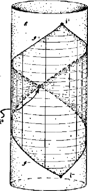
Figure 2: The embedding of Minkowski space into the Einstein cylinder $\mathcal{E}$. (This figure is taken from [11])

The characteristic feature of the dipole field is, of course, that it is a retarded field: if $p$ is such that $\ddot{p}(u)=0$ for $u\leq 0$ then no detector will see anything at times $t$ with $u=t-r\leq 0$. The information travels along the hypersurfaces $u=\mathrm{const.}$, the future light cones emanating from the world-line of the source. These are shown in fig. 1 as straight lines reaching out to $\mathcal{J}^{+}$.

What happens now if we take a detector and move it further and further out to infinity in order to extract the news function as cleanly as possible? This is not as straightforward as one would expect. The world-line of a detector is given by (ignoring the angular variables)

$$\gamma_{P}(\lambda)=(t(\lambda),r(\lambda))=(T+\lambda,R).$$

The event $P=\gamma_{P}(0)$ which characterizes the world-line of the detector uniquely can be interpreted as the event when the detector “switches on”, i.e., starts to register. We have $T=t(P)$ and $R=r(P)$. The world-line of the detector in terms of $(u,v)$-coordinates is

$$\gamma_{P}:(u(\lambda),v(\lambda))=(T-R+\lambda,T+R+\lambda)$$ (3.5)

and in terms of $(U,V)$-coordinates one has

$$\gamma_{P}:(U(\lambda),V(\lambda))=(\arctan(T-R+\lambda),\arctan(T+R+\lambda))$$ (3.6)

We take a sequence of detectors, determined by their “switch-on events” $P_{n}$ (with $T_{n}=t(P_{n})$ and $R_{n}=r(P_{n})$) such that $R_{n}\to\infty$ for $n\to\infty$. First suppose the sequence is such that $T_{n}=T=\mathrm{const}$. Then we obtain a “limiting detector”

$$\lim_{n\to\infty}\gamma_{P_{n}}(\lambda)=\lim_{n\to\infty}(U_{n}(\lambda),V_{n}(\lambda))=(-\frac{\pi}{2},\frac{\pi}{2}),$$ (3.7)

i.e., the limiting detector has been compressed entirely to the point $i^{0}$. This limit is reasonable but not useful. In fact, what happens is that the detectors switch on at the same time $t=T$. Then they have to sit and wait for the signal to arrive, the delay growing longer and longer, depending on their distance to the source, and in the limit there will be no signal at all.

Therefore, we need to use a different sequence of detectors. Operationally speaking, we trigger the detectors to switch on when the signal arrives. Thus, we have a sequence for which $T_{n}-R_{n}=u_{0}=\mathrm{const}$. Then we obtain

$$\lim_{n\to\infty}\gamma_{P_{n}}(\lambda)=\lim_{n\to\infty}(U_{n}(\lambda),V_{n}(\lambda))=(\arctan(u_{0}+\lambda),\frac{\pi}{2}).$$ (3.8)

This “limiting detector” is a line on $\mathcal{J}^{+}$ determined by the angles $\theta$ and $\phi$. Furthermore, it is a generator of $\mathcal{J}^{+}$ and, hence, a null geodesic. However, the parameter $\lambda$ is not just any parameter along that geodesic. Instead, it is a so called Bondi parameter [11]: let $s$ be an arbitrary parameter along the generator and let $\mathbf{k}=d/ds$ be the tangent vector along the generator with $\mathbf{k}(s)=1$. The acceleration $a$ of $\mathbf{k}$ is defined by the equation $d\mathbf{k}/ds=a\mathbf{k}$. Then $\lambda$ is a Bondi parameter if it satisfies the equation

$$\left(\frac{d}{ds}-a-2\rho^{\prime}\right)\frac{d\lambda}{ds}=0.$$ (3.9)

Here, $\rho^{\prime}$ is the expansion of $\mathcal{J}^{+}$, a quantity which determines how quickly neighbouring generators spread apart. It is determined intrinsically from the way $\mathcal{J}^{+}$ is attached to the physical space-time. The concept of a Bondi parameter is conformally invariant so it does not depend on which conformal factor has been used to attach the boundary to physical space. If $\lambda$ is a Bondi parameter then every other Bondi parameter has the form $G(\theta,\phi)\lambda+H(\theta,\phi)$ where $G$ and $H$ are arbitrary functions on the sphere of generators of $\mathcal{J}^{+}$.

This freedom in the choice of parameters is exactly what one would expect considering the way it was defined. Recall that we took the sequence of detectors in such a way that their world-lines were defined by keeping the spatial coordinartes fixed. However, these coordinates were one special choice of Minkowski coordinates. Any other choice would serve the same purpose. Thus, we have the freedom of the full Poincaré group available to define the detectors. The limit of these detectors will always be a generator of $\mathcal{J}^{+}$ with a Bondi parameter on it but the parameters will not be the same. Instead they will exhaust the full 2-dimensional affine space of possible Bondi parameters.

To verify that $\lambda$ is indeed a Bondi parameter in our case we observe that $U$ can be taken as a parameter along the generator. In fact, it is an affine parameter so that the corresponding acceleration vanishes. For the expansion we get $\rho^{\prime}=\tan U$. Inserting this into the equation (3.9) shows that it is identically satisfied. In fact, we may take the retarded time $u=\tan U$ itself as a Bondi parameter because it also satisfies (3.9). In order to complete the notion of a detector at infinity we observe that the radiation fields are both tangent to the spheres of constant $t$ and $r$ and this remains so even in the limit $r\to\infty$. Thus, we require that the detector at infinity has two of its axes tangent to $\mathcal{J}^{+}$ and perpendicular to the generator.

What we have found with this limiting procedure is a concept which is entirely intrinsic to $\mathcal{J}^{+}$. It does not depend anymore on the fact that we have started with Minkowski space. Instead it is a concept which can be introduced whenever the notion of null-infinity is well defined. Therefore, we now make the

Definition 1

A detector at infinity is idealized by a generator of $\mathcal{J}^{+}$ which is parametrized by a Bondi parameter $u$. The axes of the detector should be oriented so that one axis (the “retarded time” axis) coincides with $d/du$ while two other axis are perpendicular to the generator and tangent to $\mathcal{J}^{+}$.

4 Radiation extraction at infinity

Let us see whether we can now use this definition to extract radiative information. Suppose we were to solve the Maxwell equations numerically in Minkowski space. And suppose we do not use the traditional way but instead solve a conformally equivalent set of equations on a conformally related space like the Einstein cylinder $\mathcal{E}$. The Maxwell equations are conformally invariant so we still have to solve the Maxwell equations, only reexpressed in terms of the conformal metric $g$ instead of the Minkowski metric $\tilde{g}$. Of course, we have to put in somewhere that we are really interested in fields on Minkowski space and not in the more general fields on the Einstein cylinder $\mathcal{E}$. This is done by specifying the initial data appropriately.

The numerical solution of these equations provides us with a Maxwell field on the complete Einstein cylinder including that piece which corresponds to Minkowski space and its conformal boundary $\mathcal{J}^{+}$. Usually, this solution will be represented on 3-dimensional spacelike hypersurfaces which form a foliation of the conformal space. On each such slice, we can now search for the location of its intersection with $\mathcal{J}^{+}$, a 2-dimensional closed surface. Then we can evaluate the Maxwell field on that surface and so, keeping the angles fixed and going from one slice to the next, we obtain the value of the Maxwell field along a generator of $\mathcal{J}^{+}$ as a function of the time parameter which labels the slices.

As an example, we consider again the dipole fields. In order to get the solutions onto the Einstein cylinder we first write the electric and magnetic field as one-forms and then combine them into the Faraday 2-form according to

$$F=dt\wedge E+\star B.$$ (4.1)

The star is the Hodge star of the metric on the euclidean spaces $t=\mathrm{const}$. The covariant form of the fields turns out to be

$$E =\left(\ddot{p}+\frac{\dot{p}}{r}+\frac{p}{r^{2}}\right)\,\sin\theta\,d\theta+2\cos\theta\left(\frac{p}{r^{3}}+\frac{\dot{p}}{r^{2}}\right)\,dr,$$ (4.2)

$$B =\left(\ddot{p}+\frac{\dot{p}}{r}\right)\,\sin^{2}\theta\,d\phi.$$ (4.3)

In terms of the double null coordinates $u$ and $v$ we obtain

$$F=-\left(\ddot{p}+\frac{\dot{p}}{r}\right)\,du\wedge dy-\frac{p}{2r^{2}}\left(du+dv\right)\wedge dy+y\left(\frac{p}{r^{3}}+\frac{\dot{p}}{r^{2}}\right)\,du\wedge dv,$$ (4.4)

where $r=(v-u)/2$ is considered as a function of $u$ and $v$ and where we have introduced $y=\cos\theta$ as another coordinate. Observe, that the radiation field sits entirely in the $du\wedge dy$ component of $F$. It is the only component which survives the limit $r\to\infty$, keeping $u$ fixed. In the non-axisymmetric case we would also get a radiation component proportional to $du\wedge d\phi$ and this is the general behaviour for Maxwell fields on asymptotically flat space-times. This implies that we get the radiation fields from the Faraday 2-form simply by restricting it to $\mathcal{J}^{+}$.

The Faraday 2-form is conformally invariant. This implies that one gets the corresponding Faraday form on the Einstein cylinder by performing the coordinate transformation which transforms from the $u,v$ coordinates to the $U,V$ coordinates. This results in

$$F =-\left(\left(\ddot{P}-2\tan U\dot{P}\right)\cos^{2}U+2\frac{\dot{P}\cos U\cos V}{\sin(V-U)}\right)\,dU\wedge dy$$

$$-\frac{P}{2\sin^{2}(V-U)}\left(\cos^{2}VdU+\cos^{2}UdV\right)\wedge dy$$

$$+4y\left(\frac{2P\cos U\cos V}{\sin^{3}(V-U)}+\frac{\dot{P}\cos^{2}U}{\sin^{2}(V-U)}\right)\,dU\wedge dV,$$

where the function $P$ is defined by $P(U)=p(\tan U)$ and the dot here means $d/dU$.

Let us now restrict this form to $\mathcal{J}^{+}$ by pulling it back along the inclusion map $i:\mathcal{J}^{+}\to\mathcal{E},(U,y,\phi)\mapsto(U,\frac{\pi}{2},y,\phi)$

$$i^{*}F=-\left(\ddot{P}-2\tan U\dot{P}\right)\cos^{2}U\,dU\wedge dy.$$ (4.5)

According to the discussion above, this is the radiation field.

The detector at infinity is a line $y=\mathrm{const}.$ (and $\phi=\mathrm{const.}$) on $\mathcal{J}^{+}$ with a Bondi parameter on it. The variable $U$ is not a Bondi parameter. In order to find one we need to solve the second order equation (3.9). Of course, we know that $u=\tan U$ is a solution, so that the radiation field in terms of this parameter reads

$$i^{*}F=-\ddot{\tilde{p}}(u)\,du\wedge dy,$$ (4.6)

where $P(U)=\tilde{p}(\tan U)$. By comparison with the above definition of $P$ we get $p(u)=\tilde{p}(u)$. Hence, the radiation field obtained from the conformal treatment by restriction to $\mathcal{J}^{+}$ and introduction of a (special) Bondi parameter exactly reproduces the radiative information that we are interested in.

However, in most cases of interest there is no preferred Bondi parameter and then we have to regard all parameters as equivalent. To see what changes when a different parameter is used, we recall that any Bondi parameter is of the form $\bar{u}=Gu+H$. Since the shift of origin is of no consequence we choose $H=0$. Then $u=\bar{u}/G$ and

$$i^{*}F=-\frac{1}{G}\,\ddot{p}(\bar{u}/G)\,d\bar{u}\wedge dy,$$ (4.7)

so that the radiation field expressed in terms of $\bar{u}$ is $\frac{1}{G}\,\ddot{p}(\bar{u}/G)$.

In order to interpret this behaviour we have to keep in mind that the electromagnetic field has been given with respect to one specific Minkowski coordinate system. But all such systems are equivalent. Suppose we choose a new Minkowski coordinate system which is boosted with velocity $w$ with respect to the old one along the direction towards the detector. Then one finds the transformation of the retarded time to be $u\mapsto\bar{u}=\alpha u$ with $\alpha=\sqrt{(1+w)/(1-w)}$. The radiative components of the covariant fields transform according to

$${(E_{\mbox{rad}},B_{\mbox{rad}})}\mapsto{(\bar{E}_{\mbox{rad}},\bar{B}_{\mbox{rad}})}=\frac{1}{\alpha}{(E_{\mbox{rad}},B_{\mbox{rad}})}.$$ (4.8)

For $E_{\mbox{rad}}$ we then have

$$E_{\mbox{rad}}\mapsto\frac{1}{\alpha}E_{\mbox{rad}}=-\frac{1}{\alpha}\ddot{p}(u)\,dy=-\frac{1}{\alpha}\ddot{p}(\bar{u}/\alpha)\,dy$$ (4.9)

and similarly for $B_{\mbox{rad}}$. Identifying $G$ and $\alpha$ we have the same transformation law. This means that the freedom in the Bondi parameters reflects the freedom in the choice of Minkowski coordinates. Mathematically, this is to be expected and physically, this is a well known phenomenon, namely the Doppler shift in the incident signal due to the relative motion of the source and the detector. The ambiguity arises because this motion is not known a priori but has to be determined by other means (e.g., spectroscopic methods).

5 Gravitational radiation

Let us now see how the above discussion applies to the more complicated case of gravity. We have already mentioned above that the concept of the detector at infinity as stated in section 3 is entirely intrinsic to $\mathcal{J}$. It can be applied whenever there is a well-defined notion of null-infinity available. Therefore, we only need to see what corresponds to the radiative information which, in our simple example of the Maxwell case, was given by the changing dipole moment. For the following discussion we refer to the work of Janis and Newman [8] on the structure of the sources of the gravitational field. This paper contains a unified treatment of Maxwell theory and linearized gravity which is very useful for our purposes. Incidentally, these authors treat the radiation of the general multipole moments from which it becomes obvious that our discussion which was restricted to the dipole case generalizes in a straightforward way without any change in the essential statements.

We put the electromagnetic dipole field in a form which is very much like the one for the gravitational field. We introduce the Bondi frame of (complex) null vector fields

$$\mathbf{l}=2\partial_{v},\qquad\mathbf{n}=\partial_{u},\qquad\mathbf{m}=\frac{1}{\sqrt{2}r}\left(\partial_{\theta}+\frac{i}{\sin\theta}\partial_{\phi}\right).$$ (5.1)

Then we can encode the electric and magnetic fields in three complex scalar functions $\phi_{0}$, $\phi_{1}$, $\phi_{2}$ as follows:

$$\phi_{0} =F(\mathbf{l},\mathbf{m})=\frac{1}{\sqrt{2}}\frac{p}{r^{3}}\,\sin\theta,$$ (5.2)

$$\phi_{1} =\frac{1}{2}\left(F(\mathbf{l},\mathbf{n})+F(\mathbf{m},\mathbf{\bar{m}})\right)=-\left(\frac{p}{r^{3}}+\frac{\dot{p}}{r^{2}}\right)\cos\theta,$$ (5.3)

$$\phi_{2} =F(\mathbf{\bar{m}},\mathbf{n})=-\frac{1}{\sqrt{2}}\left(\frac{\ddot{p}}{r}+\frac{\dot{p}}{r^{2}}+\frac{p}{2r^{3}}\right)\sin\theta$$ (5.4)

A simple definition of $a_{1}=p/\sqrt{2}$ achieves complete agreement with the dipole field given in [8]. These authors define the coefficient $\phi_{2}^{0}(u,\theta,\phi)$ of $1/r$ in the scalar $\phi_{2}$ as the “news function”. Physically, this function is the information sent by a “broadcasting” station. Mathematically, it is one piece of the free data for the solution of the characteristic initial value problem for the Maxwell equations on Minkowski space. It is that piece of data which can be considered as being given on $\mathcal{J}^{+}$, or, physically, that component of the field which can be extracted from $\mathcal{J}^{+}$ by an infinite detector. We will also call it the “null-datum” on $\mathcal{J}^{+}$.

The similarity between the Maxwell equations and the equations for linearized gravity suggests that also in the latter case there is a “news function”. Indeed, the function in question is $\psi_{4}^{0}$, the component of the linearized Weyl spinor which is entirely intrinsic to $\mathcal{J}^{+}$. It plays the same role for the solution of the characteristic initial value problem as does the $\phi_{2}^{0}$ in the Maxwell case. Thus, in the linearized gravity case things are very much in analogy to the Maxwell case. In order to extract the radiative information one determines the null-datum $\psi_{4}^{0}$ along all the generators of $\mathcal{J}^{+}$ as a function of a Bondi parameter.

For the full theory we can again employ an analogy. The asymptotic structure of the non-linear gravitational field is very similar to that of the asymptotic linearized field. Again, one can isolate a function $\Psi_{4}^{0}$, the component of the Weyl spinor which is intrinsic to $\mathcal{J}^{+}$. This can also be given freely in the solution of the asymptotic characteristic initial value problem (see e.g., [9]). Thus, mathematically, it serves the same purpose as $\phi_{2}^{0}$ and $\psi_{4}^{0}$. However, its physical meaning is not so clear cut as before. $\Psi_{4}^{0}$ does give information about the multipole structure of the gravitational radiation but the implications for the multipole structure of the source are not as direct as they were before. The field interacts with itself due to the non-linearity of the theory, thus creating additional structure not attributable to the source. Examples of this are the critical phenomena in the scalar field collapse and the quasi-normal ringdown of perturbed black holes. Therefore, there is no direct relationship between the multipole moments of the source on the one hand and those of the gravitational radiation on the other. But irrespective of these issues, the null-datum in the non-linear theory is $\Psi_{4}^{0}$ and it is the one that contains the radiative information of the gravitational field. The “news function” for full gravity has been defined by Bondi [1]) in a different way. It is related to the null-datum $\Psi_{4}^{0}$, which is its $u$-derivative. In contrast to the null-datum which is a local quantity, the news is well defined only globally on $\mathcal{J}^{+}$ and therefore it is not as accessible as $\Psi_{4}^{0}$.

6 Discussion and conlusion

In all cases we have discussed, there is a null-datum which contains information about the structure of the field and its sources. These functions are those which can be registered on $\mathcal{J}^{+}$ by the infinite detectors. The extraction process consists of evaluating the news on $\mathcal{J}^{+}$ as a function of a Bondi parameter on all generators. Then one obtains the two polarizations of the radiation which arrives on $\mathcal{J}^{+}$. We have described an idealised extraction process and we have argued that it is a natural idealisation of the real physical measurement. Furthermore, it is a procedure which is entirely intrinsic to $\mathcal{J}^{+}$, a property which makes it very valuable within the framework of the conformal techniques in numerical relativity.

Within these methods the extraction process becomes an unambiguous algorithm which allows the determination of the well defined news function up to the freedom of the choice of an origin of time for each detector and the indeterminacy due to the unknown boost between the source and the detector. The only approximation involved is the basic assumption that the arena be an asymptotically flat space-time. In contrast to this, other extraction methods which are based on points in the finite region of space-time have to make additional assumptions in order to separate the far-field from the near-field.

We have shown in [3] that one can accurately recover the news from $\mathcal{J}^{+}$ so that the discussion of the present paper is not academic but a practical one. What remains to be tested numerically is the location of the generators of $\mathcal{J}^{+}$ on each time-slice and the determination of the Bondi parameters on them. This will be discussed in a later paper.

References

- [1] H. Bondi, M. G. J. van der Burg, and A. W. K. Metzner, Gravitational waves in general relativity. VII Waves from axi-symmetric isolated systems, Proc. Roy. Soc. London A, 269 (1962), pp. 21–52.
- [2] J. Frauendiener, Numerical treatment of the hyperboloidal initial value problem for the vacuum Einstein equations. I. The conformal field equations. to appear in Phys. Rev. D.
- [3] , Numerical treatment of the hyperboloidal initial value problem for the vacuum Einstein equations. II. The evolution equations. to appear in Phys. Rev. D.
- [4] H. Friedrich, The asymptotic characteristic initial value problem for Einstein’s vacuum field equations as an initial value problem for a first-order quasilinear symmetric hyperbolic system, Proc. Roy. Soc. London A, 378 (1981), pp. 401–421.
- [5] S. Hawking and G. F. R. Ellis, The large scale structure of space-time, Cambridge University Press, Cambridge, 1973.
- [6] P. Hübner, Black hole spacetimes on grids with trivial boundaries. preprint AEI-062,gr-qc/9804065.
- [7] J. D. Jackson, Classical Electrodynamics, John Wiley & Sons, New York, 1975.
- [8] A. I. Janis and E. T. Newman, Structure of gravitational sources, J. Math. Phys., 6 (1965), pp. 902–914.
- [9] E. T. Newman and T. W. J. Unti, Behavior of asymptotically flat empty space, J. Math. Phys., 3 (1962), pp. 891–901.
- [10] R. Penrose, Zero rest-mass fields including gravitation: asymptotic behaviour, Proc. Roy. Soc. London A, 284 (1965), pp. 159–203.
- [11] R. Penrose and W. Rindler, Spinors and Spacetime, vol. 2, Cambridge University Press, Cambridge, 1986.
- [12] A. Sommerfeld, Vorlesungen über Theoretische Physik, Band III. Elektrodynamik, Verlag Harri Deutsch, Thun, 4. ed., 1977. reprint.