Abstract

I start with a discussion of the no-hair principle. The hairy black hole solutions of recent vintage do not deprive it of value because they are often unstable. Generic properties of spherical static black holes with nonvacuum exteriors are derived. These form the basis for the discussion of the new no scalar hair theorems. I discuss the generic phenomenon of superradiance for its own sake, as well as background for black hole superradiance. First I go into uniform linear motion superradiance with some examples. I then discuss Kerr black hole superradiance in connection with a general rotational superradiance theory with possible applications in the laboratory. Adiabatic invariants have played a weighty role in theoretical physics. I explain why the horizon area of a nearly stationary black hole can be regarded as an adiabatic invariant, and support this by examples as well as a general discussion of perturbations of the horizon. The horizon area’s adiabatic invariance suggests that its quantum counterpart is quantized in multiples of a basic unit. Consideration of the quantum analog of the Christodoulou reversible processes provides support for this idea. Area quantization provides a definite discrete black hole mass spectrum. Black hole spectroscopy follows: the Hawking semiclassical spectrum is replaced by a spectrum of nearly uniformly spaced lines whose envelope may be roughly Planckian. I estimate the lines’ natural broadening. To check on the possibility of line splitting, I present a simple algebra involving, among other operators, the black hole observables. Under simple assumptions it also leads to the uniformly spaced area spectrum.
In these lectures I take units for which $c=1$. Occasionally, where mentioned explicitly, I also set $G=1$, but always display $\hbar$.

Black Holes: Classical Properties, Thermodynamics,
and Heuristic Quantization

¹Racah Institute of Physics, Hebrew University of Jerusalem,
Givat Ram, 91904 Jerusalem, ISRAEL

1 No scalar hair theorems

Almost thirty years ago Wheeler enunciated the Israel-Carter conjecture, today colloquially known as “black holes have no hair” [88]. This influential conjecture has long been regarded as a theorem by large sectors of the gravity-particle physics community. But by the early 1990’s solutions for stationary black holes with exterior nonabelian gauge or skyrmion fields [105, 27, 39, 62, 44] had led many workers to regard the conjecture as having fallen by the wayside. By now things have settled down to a new paradigm not very different from Wheeler’s original one.

1.1 Early days of ‘no-hair’

By 1965 the charged Kerr-Newman black hole metric was known. Inspired by Israel’s uniqueness theorems for the Schwarzschild and Reissner-Nordström black holes [52], and by Carter’s [33] and Wald’s [106] uniqueness theorems for the Kerr black hole, Wheeler anticipated that “collapse leads to a black hole endowed with mass and charge and angular momentum, but, so far as we can now judge, no other free parameters” by which he meant that collapse ends with a Kerr-Newman black hole. Wheeler stressed that other ‘quantum numbers’ such as baryon number or strangeness can have no place in the external observer’s description of a black hole.

What is so special about mass, electric charge and angular momentum ? They are all conserved quantities subject to a Gauss type law. One can thus determine these properties of a black hole by measurements from afar. Obviously this reasoning has to be completed by including magnetic (monopole) charge as a fourth parameter because it also is conserved in Einstein-Maxwell theory, it also submits to a Gauss type law, and duality of the theory permits Kerr-Newman like solutions with magnetic charge alongside (or instead of) electric charge. In the updated version of Wheeler’s conjecture, the forbidden “hair” is any field not of gravitational or electromagnetic nature associated with a black hole.

But why is the issue of hair interesting ? Black holes are in a real sense gravitational solitons; they play in gravity theory the role atoms played in the nescent quantum theory of matter and chemistry. Black hole mass and charge are analogous to atomic mass and atomic number. Thus if black holes could have other parameters, such ‘hairy’ black holes would be analogous to excited atoms and radicals, the stuff of exotic chemistry. By contrast, the absence of a large number of hair parameters would support the conception of simple black hole exteriors, a situation which is natural for the formulation of black hole entropy as the measure of the vast number of hidden degrees of freedom of a black hole. Indeed, historically, the no-hair conjecture inspired the formulation of black hole thermodynamics (for the early history see review [17]), which has in the interim become a pillar of gravity theory.

Originally “no-hair theorems” meant theorems like Israel’s or Carter’s [52, 33] on the uniqueness of the Kerr-Newman family within the Einstein-Maxwell theory or like Chase’s [34] on its uniqueness within the Einstein-massless scalar field theory. Wheeler’s conjecture that baryon and like numbers cannot be specified for a black hole set off a longstanding trend in the search for new no-hair theorems. Thus Hartle [45] as well as Teitelboim [98] proved that the nonelectromagnetic force between two “baryons” or “leptons” resulting from exchange of various force carriers would vanish if one of the particles was allowed to approach a black hole horizon. I developed an alternative and very simple approach [11] to show that classical massive scalar or vector fields cannot be supported at all by a stationary black hole exterior, making it impossible to infer any information about their sources in the black hole interior.

In modernized form this goes as follows. Start with the action

$$S_{\psi}=-{\scriptstyle 1\over\scriptstyle 2}\int[\psi_{,\alpha}\psi^{,\alpha}+V(\psi^{2})](-g)^{1/2}\,d^{4}x$$ (1.1)

for a static real scalar field $\psi$. From it follows the field equation

$$\psi_{,\alpha}{}^{;\alpha}-\psi V^{\prime}(\psi^{2})=0$$ (1.2)

Assume that the configuration is asymptotically flat and stationary: $\partial\psi/\partial x^{0}=0$, where $x^{0}$ is a timelike variable in the black hole exterior. Multiply Eq. (1.2) by $\psi$ and integrate over the black hole exterior at a given $x^{0}$ (space ${\cal V}$). Integration by parts leads to

$$-\int_{\cal V}[g^{ab}\psi_{,a}\psi_{,b}+\psi^{2}V^{\prime}(\psi^{2})](-g)^{1/2}\,d^{3}x+\oint_{\partial{\cal V}}\psi\psi^{,\alpha}d\Sigma_{\alpha}=0$$ (1.3)

where $d\Sigma_{\alpha}$ is the 2-D element of the boundary hypersurface $\partial{\cal V}$. The indices $a$ and $b$ run over the space coordinates only, so that the restricted metric $g^{ab}$ is positive definite in the black hole exterior.

Now suppose the boundary ${\partial{\cal V}}$ is taken as a large sphere at infinity over all time (topology $S^{2}\times R$) together with a surface close to the horizon ${\cal H}$, also with topology $S^{2}\times R$. Then so long as $\psi$ decays as $1/r$ or faster at large distances ($r$ is the usual Euclidean distance), which will be true for static solutions of Eq. (1.2), infinity’s contribution to the boundary vanishes. At the inner boundary we can use Schwarz’s inequality to state that at every point $|\psi\psi^{,\alpha}d\Sigma_{\alpha}|\leq(\psi^{2}\,\psi^{,\alpha}\psi_{,\alpha}\ d\Sigma^{\beta}\,d\Sigma_{\beta})^{1/2}$. As the boundary is pushed to the horizon (a null surface), $d\Sigma^{\beta}\,d\Sigma_{\beta}$ must necessarily tend to zero. Thus the inner boundary term will also vanish unless $\psi^{2}\,\psi^{,\alpha}\psi_{,\alpha}$ blows up at ${\cal H}$. But this last eventuality is usually unacceptable for a black hole. Finiteness of the physical scalars $T_{\alpha\beta}T^{\alpha\beta}$ and $(T_{\alpha}{}^{\alpha})^{2}$ at ${\cal H}$ tells us that $\psi^{,\alpha}\psi_{,\alpha}$ and $V$ are both bounded at ${\cal H}$. Then if $V$ diverges for large arguments, $\psi$ has to remain bounded, and so $\psi^{2}\,\psi^{,\alpha}\psi_{,\alpha}$ is bounded on ${\cal H}$. But even if $V(\infty)\neq\infty$ so that $\psi$ is allowed to diverge, this will almost certainly cause $\psi^{,\alpha}\psi_{,\alpha}$ to diverge. In either case the boundary term vanishes.

Thus for a generic $V$ we conclude that the 4-D integral in Eq. (1.3) must itself vanish. In the case that $V^{\prime}(\psi^{2})$ is everywhere nonnegative and vanishes only at some discrete values $\psi_{j}$, then it is clear that the field $\psi$ must be constant everywhere outside the black hole, taking on one of the values $\{0,\psi_{j}\}$. The scalar field is thus trivial, either vanishing or taking a constant value as dictated by spontaneous symmetry breaking without the black hole ! In particular, the theorem works for the Klein-Gordon field for which $V^{\prime}(\psi^{2})=\mu^{2}$ where $\mu$ is the field’s mass. In that case $\psi=0$ outside the black hole [11]. Obviously the theorem supports Wheeler’s original conjecture by ruling out black hole parameters having to do with a scalar field.

One advantage of this type of theorem, in contrast with, say, Chase’s, is that it makes no use of the gravitational field equations. The inference that there are no black holes with scalar hair is thus just as true in other metric theories of gravity. Another plus is that the theorem is easily generalizable to exclude massive vector (Proca) field hair [11]. Because of both features this type of theorem was the state of the art for many years (see for instance Heusler’s monograph [51]). But this should not blind us to its shortcomings. For example, it does not rule out hair in the form of a Higgs field with a ‘Mexican hat’ potential, a darling of particle physicists. For the Higgs field $V^{\prime}(\psi^{2})$ is negative in some regime of $\psi$, and the theorem fails. This gap in the no-hair theorems remained until fairly late in the subject, as certified by Gibbons’ relatively recent review [41]).

1.2 Hairy black holes ?

When one removes the massive vector field’s mass, gauge invariance sets in and the fundamental field, basically the covariant time component of $A_{\alpha}$ (the electromagnetic 4-potential), cannot be required to be bounded at the horizon because it is not gauge invariant. No no-hair theorem can be proved: a black hole can have an electromagnetic field as witness the Kerr-Newman family. By the same logic I concluded [9] that the gauge invariance of the nonabelian gauge theories should likewise allow one or more of the gauge field components generated by sources in a black hole to “escape” from it. Thus gauge fields around a black hole may be possible in every gauge theory. Early on Yasskin  [108] exhibited some trivial hairy black holes in nonabelian gauge theories. Volkov and Gal’tsov discovery in 1989 of more interesting black hole solutions with nonabelian gauge field [105, 27] took everybody by surprise. But it obviously should not have done so !

Actually an hairy black hole was known well before. It is a solution of the action for a scalar nonminimally coupled to gravity:

$$S=S_{\rm E}+S_{\rm M}-{\scriptstyle 1\over\scriptstyle 2}\int{\left[\psi_{,\alpha}\psi^{,\alpha}+\xi R\psi^{2}+V(\psi^{2})\right]\sqrt{-g}\,d^{4}x}.$$ (1.4)

Here $S_{\rm E}$ stands for the Einstein-Hilbert action, $S_{\rm M}$ for the Maxwell one, $R$ is the Ricci curvature scalar and $\xi$ measures the strength of the coupling to the curvature. One derives the energy-momentum tensor

$$T_{\mu\nu}=\psi_{,\mu}\psi_{,\nu}-{\scriptstyle 1\over\scriptstyle 2}\psi_{,\alpha}\psi^{,\alpha}\,g_{\mu\nu}-\xi\,\psi\psi_{,\mu;\nu}+\xi\,\hbox{\hbox to0.0pt{$\sqcap$\hss}$\sqcup$}\psi^{2}\,g_{\mu\nu}+\xi\,\psi^{2}G_{\mu\nu}-{\scriptstyle 1\over\scriptstyle 2}Vg_{\mu\nu}+T_{\mu\nu}^{\rm(M)}$$ (1.5)

Substituting $G_{\mu\nu}=8\pi GT_{\mu\nu}$ turns this into

$$T_{\mu}{}^{\nu}={\psi_{,\mu}\psi^{,\nu}-{\scriptstyle 1\over\scriptstyle 2}\psi_{,\alpha}\psi^{,\alpha}\,\delta_{\mu}{}^{\nu}-\xi\,\psi\psi_{,\mu}{}^{;\nu}+\xi\,\hbox{\hbox to0.0pt{$\sqcap$\hss}$\sqcup$}\psi^{2}\,\delta_{\mu}{}^{\nu}-{\scriptstyle 1\over\scriptstyle 2}Vg_{\mu}{}^{\nu}+T^{(M)}{}_{\mu}{}^{\nu}\over 1-8\pi G\xi\psi^{2}}$$ (1.6)

For the conformally invariant coupling $\xi=1/6$ with $V=0$, Bocharova, Bronnikov and Melnikov (BBM)  [28] and independently I [14] found a black hole solution:

$$ds^{2} = -(1-GM/r)^{2}dt^{2}+(1-GM/r)^{-2}dr^{2}+r^{2}(d\theta^{2}+\sin^{2}\theta\,d\phi^{2})$$

$$F_{\mu\nu} = Q\,r^{-2}\,(\delta_{\mu}^{r}\delta_{\nu}^{t}-\delta_{\mu}^{t}\delta_{\nu}^{r});\qquad Q<\surd GM$$ (1.7)

$$\psi = \pm(3\surd G/4\pi)(M^{2}-G^{-1}Q^{2})^{1/2}(r-GM)^{-1}$$

$M$ and $Q$ are free parameters corresponding to the mass and charge of the solution. Note that the metric is an extreme Reissner-Nordström metric and that the scalar field blows up at $r=GM$, the location of the geometry’s horizon.

I interpreted this solution as genuine black hole [16] because the apparent singularity of $\psi$ at the horizon has no deleterious consequences. The invariants $T_{\alpha\beta}T^{\alpha\beta}$ and $(T_{\alpha}{}^{\alpha})^{2}$ are bounded even at ${\cal H}$ and a particle, even one coupled to $\psi$, encounters no infinite tidal forces upon approaching the horizon. Because $M$ and $Q$ are the only independent parameters, with the scalar field introducing merely a sign choice, I was not alarmed by the threat posed to no-hair by this solution. Indeed in one of his last papers before his tragic death, B. Xanthopoulos in cooperation with Zannias [107], and then Zannias alone [109] proved that there is no nonextremal extension of the BBM black hole which might have introduced a scalar charge as an extra parameter. The situation is not qualitatively changed by the addition of magnetic charge [103].

Sudarsky and Zannias [97] have lately claimed that Eqs. (1.7) are not really a solution of the action (1.4). Their point is that (for $Q=0$) although $T_{\alpha}{}^{\beta}$ is finite at ${\cal H}$, if one “regularizes” $\psi$ so that it becomes actually bounded on ${\cal H}$, the resulting finite $T_{\alpha}{}^{\beta}$ does not generate, through Einstein’s equations the metric (1.7a). The argument is rather odd as it creates a problem (regularizes $\psi$ when $T_{\alpha}{}^{\beta}$ is perfectly finite anyway) in order to solve it. However, the BBM solution has been shown to be unstable in linearized theory by Bronnikov (one of its discoverers) and Kireyev [30]. A poor man’s way of understanding why can be had by contemplating Eq. (1.6) for the energy momentum tensor. Addition of a bit of matter at the point where the denominator vanishes (which must be outside the horizon since $\psi^{2}$ blows up at the horizon) would obviously lead to a drastic perturbation in the geometry. So the solution (1.7) is unstable. Only to a purist would an unstable solution require further discussion, and there hardly seems to be any need to criticize it on another account.

In fact almost all known hairy black holes in $3+1$ general relativity are known to be unstable [95, 29, 72]. The only one which is certified to be stable [50], at least in linearized theory, is the Skyrmion hair black hole [39]. It differs from the Schwarzschild one in that it involves a parameter with properties of a topological winding number. This is not an additive quantity among several black holes, so that the Skyrmion black hole may not represents a true exception to Wheeler’s principle; however, I shall not try to reach a veredict here.

Because gauge fields seem to produce unstable hairy black holes, one should look for possible violations of no-hair in the only other direction left: scalar hair. Thus I proposed [21] to shift emphasis to the “no scalar hair” conjecture which I will state as: there are no asymptotically flat, stationary and stable black hole solutions in $3+1$ general relativity which are endowed with scalar fields. The asymptotic flatness requirement is introduced to rule out the black holes in de Sitter background  [31] as well as the Achucarro-Gregory-Kuijken black hole  [1], a charged black hole transfixed by a Higgs local cosmic string. The stability restriction is to exclude the BBM black hole. This shift has also been urged by Núñez, Quevedo and Sudarsky  [81] on the grounds that there are ‘hairy’ solutions (never mind that they are unstable) and that the hair they sport is never ‘short’ and ignorable.

Consider the case of a theory governed by action (1.4). How to prove that scalar hair is excluded even when the assumption $V^{\prime}>0$ of Sec. 1.1 is not made ? By 1995 new techniques to overcome this problem had been introduced by Heusler [49], Sudarsky [96] and myself  [18]. These led to various no scalar hair theorems for spherical black holes and minimally coupled fields. As background for these and their natural extension, I will now go into the generic properties of spherically symmetric stationary black holes with nonvacuum exteriors.

1.3 Properties of stationary spherical black holes

For a spherically symmetric and stationary black hole with any kind of matter and fields in its exterior, the metric may be taken as

$$ds^{2}=-e^{\nu}dt^{2}+e^{\lambda}dr^{2}+r^{2}(d\theta^{2}+\sin^{2}\theta\,d\phi^{2})$$ (1.8)

Here $\nu=\nu(r)$ and $\lambda=\lambda(r)$ with both behaving as $1/r$ for $r\rightarrow\infty$ (asymptotic flatness). The event horizon is at $r=r_{\cal H}$ with $r_{\cal H}$ being the outermost zero of $e^{-\lambda}$. To see why define a family of hypersurfaces with $S^{2}\times R$ topology by the conditions $\{\forall t;r=\mbox{\rm const.}\}$. Each value of the constant labels a different surface. The normal to each such hypersurface is $\eta_{\alpha}=r_{,\alpha}=\delta_{\alpha}{}^{r}$, so that $\eta_{\alpha}\eta^{\alpha}=e^{-\lambda}$ which vanishes at $r=r_{\cal H}$, but never outside it. This must thus be location of the horizon which is defined as a null surface (hence null normal).

Now in order for the black hole solution to be physical, invariants such as $T_{\alpha}{}^{\alpha}$ and $T_{\alpha\beta}\,T^{\alpha\beta}$ must be bounded throughout its exterior $r\geq r_{\cal H}$. In the coordinates of the metric (1.8) $T_{\alpha\beta}\,T^{\alpha\beta}=(T_{t}{}^{t})^{2}+(T_{r}{}^{r})^{2}+(T_{\theta}{}^{\theta})^{2}+(T_{\varphi}{}^{\varphi})^{2}$ so that $T_{r}{}^{r}$ and $T_{t}{}^{t}$ must be finite for $r\geq r_{\cal H}$.

Let me now introduce two of Einstein’s equations:

$$e^{-\lambda}(r^{-2}-r^{-1}\lambda^{\prime})-r^{-2} = 8\pi GT_{t}{}^{t},$$ (1.9)

$$e^{-\lambda}(r^{-2}+r^{-1}\nu^{\prime})-r^{-2} = 8\pi GT_{r}{}^{r}.$$ (1.10)

It follows from the second that $e^{\nu}$ also has its outermost zero at $r_{\cal H}$ (Vishveshwara’s theorem [102]). For assume that $e^{\nu}$ vanishes at some point $\bar{r}$. Then $\nu\rightarrow-\infty$ and $\nu^{\prime}\rightarrow\infty$ as $r\rightarrow\bar{r}$ from the right. It is then obvious from Eq. (1.10) that $e^{-\lambda}$ must vanish as $r\rightarrow\bar{r}$ since $T_{r}{}^{r}$ must be bounded. But since as we move in from infinity, $e^{-\lambda}$ first vanishes at $r=r_{\cal H}$, we see that $\bar{r}=r_{\cal H}$. The converse is also true: the horizon $r=r_{\cal H}$ must always be an infinite redshift surface with $e^{\nu}=0$. For if $e^{\nu}$ were positive at $r=r_{\cal H}$, then according to the metric (1.8) the $t$ direction would be timelike there, while the $\theta$ and $\phi$ directions would be, as always, spacelike. But since the horizon is a null surface, it must have a null tangent direction, and by time symmetry this must obviously be the $t$ direction. Thus it is inconsistent to assume that $e^{\nu}\neq 0$ at $r=r_{\cal H}$.

Eq. (1.9) may be integrated to get

$$e^{-\lambda}=1-{r_{\cal H}\over r}+{8\pi G\over r}\int^{r}_{r_{\cal H}}T_{t}{}^{t}r^{2}dr$$ (1.11)

The constant of integration has been adjusted so that $e^{-\lambda}$ vanishes at $r_{\cal H}$. Obviously $T_{t}{}^{t}$ must vanish asymptotically faster than $1/r^{3}$ in order for $e^{\lambda}$ not to diverge at infinity. Since $T_{t}{}^{t}$ must be bounded on the horizon, we may write the first approximation (in Taylor’s sense) near the horizon

$$e^{-\lambda}=L(r-r_{\cal H})+{\cal O}((r-r_{\cal H})^{2});\qquad L\equiv r_{\cal H}{}^{-1}+8\pi G\,r_{\cal H}\,T_{t}{}^{t}(r_{\cal H})$$ (1.12)

or

$$\lambda={\rm const.}-\ln(r-r_{\cal H})+{\cal O}(r-r_{\cal H})$$ (1.13)

Since $e^{-\lambda}$ must be nonnegative outside the horizon, we learn that $L\geq 0$, or

$$-(8\pi Gr_{\cal H}{}^{2})^{-1}\leq T_{t}{}^{t}(r_{\cal H})$$ (1.14)

so that at every stationary spherically symmetric event horizon, the energy density, if positive, is limited by the very condition of regularity. The inequality is saturated for the extremal black hole.

Eqs. (1.9-1.10) combine to the equation

$$e^{-\lambda}(\nu^{\prime}+\lambda^{\prime})=-8\pi G(T_{t}{}^{t}-T_{r}{}^{r})r.$$ (1.15)

with integral

$$\nu+\lambda=8\pi G\int^{\infty}_{r}r^{\prime}(T_{t}{}^{t}-T_{r}{}^{r})e^{\lambda}dr^{\prime}$$ (1.16)

We have built in the asymptotic requirement $\nu+\lambda\rightarrow 0$ by appropriate choice of the limits of integration. Obviously in addition to the asymptotic condition on $T_{t}{}^{t}$, $T_{r}{}^{r}$ must decrease at least as fast as $1/r^{3}$ so that the integral converges and $\nu+\lambda$ is well defined. By following the method leading to Eq. (1.12) and using that expression for $e^{-\lambda}$ we can get from Eq. (1.16)

$$\nu+\lambda={\rm const.}-8\pi Gr_{\cal H}{}^{2}\ {T_{t}{}^{t}(r_{\cal H})-T_{r}{}^{r}(r_{\cal H})\over 1+8\pi GT_{t}{}^{t}(r_{\cal H})r_{\cal H}{}^{2}}\ln(r-r_{\cal H})+{\cal O}(r-r_{\cal H})$$ (1.17)

which in view of Eq. (1.13) gives

$$\nu={\rm const.}+\beta\ln(r-r_{\cal H})+{\cal O}(r-r_{\cal H});\qquad\beta\equiv{1+8\pi GT_{r}{}^{r}(r_{\cal H})r_{\cal H}{}^{2}\over 1+8\pi GT_{t}{}^{t}(r_{\cal H})r_{\cal H}{}^{2}}$$ (1.18)

The value of $\beta$ is restricted by the requirement that the scalar curvature

$$R=e^{-\lambda}\left(\nu^{\prime\prime}+{\scriptstyle 1\over\scriptstyle 2}\nu^{\prime 2}+{2\over r}(\nu^{\prime}-\lambda^{\prime})-{\scriptstyle 1\over\scriptstyle 2}\nu^{\prime}\lambda^{\prime}+{2\over r^{2}}\right)-{2\over r^{2}}$$ (1.19)

be bounded on the horizon (this is the same as boundedness of $T_{\alpha}{}^{\alpha}$). If we substitute here Eqs. (1.13) and (1.18) we get

$$R=-{2\over r_{\cal H}{}^{2}}+L\ (r-r_{\cal H})\times\left({\scriptstyle 1\over\scriptstyle 2}{\beta(\beta-1)\over(r-r_{\cal H})^{2}}+{2\over r_{\cal H}}{\beta+1\over(r-r_{\cal H})}+{2\over r_{\cal H}{}^{2}}\right)$$ (1.20)

For a nonextremal black hole $L>0$, so we are left with the condition

$$\beta(\beta-1)=0$$ (1.21)

The alternative $\beta=0$ is excluded by the requirement that $e^{\nu}=0$ at the horizon. Thus necessarily $\beta=1$. It follows from Eq. (1.18) that

$$T_{t}{}^{t}=T_{r}{}^{r}\quad{\rm at}\quad r=r_{\cal H}$$ (1.22)

$$e^{\nu}=N(r-r_{\cal H})+{\cal O}((r-r_{\cal H})^{2})$$ (1.23)

where $N$ denotes a positive constant. Equality (1.22), which has been derived by several groups [1, 81, 73], can also be proved for extremal black holes; the factors in $(r-r_{\cal H})$ in Eqs. (1.12) and (1.23) are then replaced by $(r-r_{\cal H})^{2}$ [73].

1.4 No minimally coupled scalar hair

Consider a black hole solution of the theory whose action is

$$S=S_{\rm E}-\int{\cal E}({\cal I},\psi)\sqrt{-g}\,d^{4}x;\qquad{\cal I}\equiv g^{\alpha\beta}\psi_{,\alpha}\psi_{,\beta}$$ (1.24)

where ${\cal E}$ is some function. I have dropped the Maxwell action (so that I only consider electrically neutral black holes), but for later convenience have generalized the scalar action. The scalar’s energy momentum tensor turns out to be

$$T_{\mu}{}^{\nu}=2\partial{\cal E}/\partial{\cal I}\ \psi_{,\mu}\psi^{,\nu}-{\cal E}\delta_{\mu}{}^{\nu}$$ (1.25)

Of course not every function ${\cal E}$ leads to a physical theory. It is reasonable to restrict attention to fields that bear locally positive energy density as seen by any physical observer. Unless ${\cal E}>0$ and $\partial{\cal E}/\partial{\cal I}>0$ for any $\psi$ and ${\cal I}>0$, some observer (represented by its 4-velocity $u^{\mu}$) will see negative energy density $T_{\mu\nu}u^{\mu}u^{\nu}$ somewhere in a stationary scalar field configuration. Thus we assume ${\cal E}>0$ and $\partial{\cal E}/\partial{\cal I}>0$. The action (1.4) with $\xi=0$ is just (1.24) with ${\cal E}={\scriptstyle 1\over\scriptstyle 2}\left[{\cal I}+V(\psi^{2})\right]$ and satisfies both conditions provided $V$ is positive definite. In fact, any potential bounded from below will do because one can add a suitable constant to it to make it nonnegative.

Are there spherically symmetric stationary black hole solutions of the action (1.24) [18] ? The $r$ component of the energy-momentum conservation law $T_{\mu}{}^{\nu}{}_{;\nu}=0$ takes the form [58]

$$[(-g)^{1/2}\,T_{r}{}^{r}]^{\prime}-{\scriptstyle 1\over\scriptstyle 2}(-g)^{1/2}\,(g_{\alpha\beta})^{\prime}T^{\alpha\beta}=0,$$ (1.26)

where ${}^{\prime}\equiv\partial/\partial r$. Because of the stationarity and spherical symmetry, $T_{\mu}{}^{\nu}{}$ must be diagonal and $T_{\theta}{}^{\theta}=T_{\varphi}{}^{\varphi}$. These conditions allow us to rewrite Eq. (1.26) in the form

$$(e^{\lambda+\nu\over 2}r^{2}T_{r}{}^{r})^{\prime}-{\scriptstyle 1\over\scriptstyle 2}e^{\lambda+\nu\over 2}r^{2}\left[\nu^{\prime}T_{t}{}^{t}+\lambda^{\prime}T_{r}{}^{r}+4T_{\theta}{}^{\theta}/r\right]=0.$$ (1.27)

The terms containing $\lambda^{\prime}$ cancel out so that

$$(e^{\nu/2}r^{2}T_{r}{}^{r})^{\prime}={\scriptstyle 1\over\scriptstyle 2}e^{\nu/2}r^{2}\left[\nu^{\prime}T_{t}{}^{t}+4T_{\theta}{}^{\theta}/r\right].$$ (1.28)

Eq. (1.25) and the symmetries show that $T_{t}{}^{t}=T_{\theta}{}^{\theta}=-{\cal E}$. Substituting this in the r.h.s. of Eq. (1.28) and rearranging the derivatives we get our key expression

$$(e^{\nu/2}r^{2}T_{r}{}^{r})^{\prime}=-(e^{\nu/2}r^{2})^{\prime}{\cal E}.$$ (1.29)

Let us now integrate Eq. (1.29) from $r=r_{\cal H}$ to a generic $r$. The boundary term at the horizon vanishes because $e^{\nu}=0$ and $T_{r}{}^{r}$ is finite there. We get

$$T_{r}{}^{r}(r)=-{e^{-\nu/2}\over r^{2}}\int_{r_{\cal H}}^{r}{(r^{2}e^{\nu/2})^{\prime}\,{\cal E}}dr.$$ (1.30)

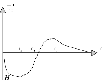
Figure 1: Energy momentum conservation reveals the shape of $T_{r}{}^{r}$ vs. $r$ near the horizon $H$ and asymptotically; continuity requires us to complete the curve so that it rises as well as crosses the $r$ axis.

Now, since $e^{\nu}$ vanishes at $r=r_{\cal H}$ and must be positive outside it, $r^{2}e^{\nu/2}$ must grow with $r$ sufficiently near the horizon. It is then immediately obvious from Eq. (1.30) and the positivity of ${\cal E}$ that sufficiently near the horizon, $T_{r}{}^{r}<0$ (see Fig. 1).

Further, carry out the differentiation in Eq. (1.29) and rearrange terms to get

$$(T_{r}{}^{r})^{\prime}=-e^{-\nu/2}r^{-2}\,(r^{2}e^{\nu/2})^{\prime}\,({\cal E}+T_{r}{}^{r}).$$ (1.31)

From Eq. (1.25) we obtain

$${\cal E}+T_{r}{}^{r}=2e^{-\lambda}(\partial{\cal E}/\partial{\cal I})\psi_{,r}^{2}$$ (1.32)

This is positive by our assumptions. It then follows from Eq. (1.31) and our previous conclusion about $r^{2}e^{\nu/2}$ that sufficiently near the horizon $(T_{r}{}^{r})^{\prime}<0$ as well.

Since asymptotically $e^{\nu/2}\rightarrow 1$, Eq. (1.31) also tells us that $(T_{r}{}^{r})^{\prime}<0$ asymptotically. We mentioned already in connection with Eq. (1.11) that $T_{t}{}^{t}=-{\cal E}$ must decrease asymptotically faster than $r^{-3}$ to guarantee asymptotic flatness of the solution. Thus the integral in Eq. (1.30) converges and $|T_{r}{}^{r}|$ decreases asymptotically as $r^{-2}$. But since $(T_{r}{}^{r})^{\prime}<0$ asymptotically, we deduce that $T_{r}{}^{r}$ must be positive and decreasing with increasing $r$ as $r\rightarrow\infty$, as depicted in Fig. 1. Now we found that near the horizon $T_{r}{}^{r}<0$ and $(T_{r}{}^{r})^{\prime}<0$. All these facts together tell us that in some intermediate interval $[r_{\rm a},r_{\rm b}]$, $(T_{r}{}^{r})^{\prime}>0$ and also that $T_{r}{}^{r}$ itself changes sign at some $r_{\rm c}$, with $r_{\rm a}<r_{\rm c}<r_{\rm b}$, being positive in $[r_{\rm c},r_{\rm b}]$ (see Fig. 1; there may be several such intervals $[r_{\rm a},r_{\rm b}]$). Well, it turns out that this conclusion is incompatible with the Einstein equations, to which we now turn.

First we note from Eq. (1.11) that $e^{\lambda}\geq 1$ throughout the black hole exterior (recall $T_{t}{}^{t}=-{\cal E}<0$). Next we recast Eq. (1.10) in the form

$$e^{-\nu/2}r^{-2}\,(r^{2}e^{\nu/2})^{\prime}=[4\pi rGT_{r}{}^{r}+(1/2r)]e^{\lambda}+3/2r>4\pi rGT_{r}{}^{r}e^{\lambda}+2/r,$$ (1.33)

where the inequality results because $e^{\lambda}/2+3/2>2$. We found that in $[r_{\rm c},r_{\rm b}]$, $T_{r}{}^{r}>0$. Thus $e^{-\nu/2}r^{-2}\,(r^{2}e^{\nu/2})^{\prime}>0$ there. According to Eq. (1.31) this means that $(T_{r}{}^{r})^{\prime}<0$ throughout $[r_{\rm c},r_{\rm b}]$. However, we determined that $(T_{r}{}^{r})^{\prime}>0$ throughout the encompassing interval $[r_{\rm a},r_{\rm b}]$. Thus there is a contradiction: the solution as we have been imagining it does not exist.

To escape the contradiction we must have $T_{r}{}^{r}=0$ identically in the black hole exterior. According to Eq. (1.29) this implies that ${\cal E}=0$ identically. It then follows from Eq. (1.32) that $\psi$ must be constant throughout the black hole exterior, taking on a value which makes $T_{\mu\nu}=0$. Such a values must exist in order that a trivial solution of the scalar equation be possible in Minkowski spacetime. It is precisely this solution which served as an asymptotic boundary condition in our argument. By Birkhoff’s theorem the spherical stationary black hole solution of action (1.24) must be identically Schwarzschild. This rules out hair in the form of a neutral minimally coupled scalar field. This result can be generalized to many scalar fields  [18].

The advantage of this theorem [18] and those of Heusler [49] and Sudarsky [96] over the older one of Sec. 1.1 is that now we can rule neutral Higgs hair provided only $V\geq 0$, without need to invoke $V^{\prime}>0$ which is often violated in field theoretic models. A disadvantage is that the present theorems work only for spherical symmetry, and do make use of Einstein’s equations. However, the theorem just described has been extended to the Brans-Dicke theory [18] (see also Ayon’s work [6]), as well as to electrically charged black holes [73]. Removal of the static and spherical symmetry assumptions is a thing for the future; some headway has been reported by Ayon [5].

1.5 No curvature coupled scalar hair

Consider now a hairy spherically symmetric stationary black hole solution of the action (1.4) with $\xi\neq 0$ (curvature coupled), and with $V\geq 0$ but no electric charge. The curvature coupled field’s energy density is not necessarily positive definite. Thus I drop the requirement of positive energy density, but I shall look only at positive $V$ so that a suitable limit can be taken to the minimally coupled theory discussed earlier. In addition, I shall assume the physical black hole configurations are such that the dominant energy condition [47] is satisfied everywhere. This means the absolute value of the energy density bounds all the other components of the energy-momentum tensor.

Both Saa [89, 90] and Mayo and I [73] realized that this problem can be mapped onto the one solved in Sec. 1.4 by a conformal transformation of the geometry.

$$g_{\mu\nu}\rightarrow\bar{g}_{\mu\nu}\equiv g_{\mu\nu}\Omega;\quad\Omega\equiv 1-8\pi G\xi\psi^{2}$$ (1.34)

Under this map the action (1.4) is transformed into

$$S = {1\over 16\pi G}\int{\bar{R}\sqrt{-\bar{g}}d^{4}x}-{\scriptstyle 1\over\scriptstyle 2}\int{\left[(1+f)\bar{g}^{\alpha\beta}\psi_{,\alpha}\psi_{,\beta}+\bar{V}\right]\sqrt{-\bar{g}}d^{4}x}$$

$$f \equiv 48\pi G\xi^{2}\psi^{2}(1-8\pi G\xi\psi^{2})^{-2}$$

$$\bar{V} \equiv V(\psi^{2})(1-8\pi G\xi\psi^{2})^{-2}$$ (1.35)

The transformed action is of the form (1.24), and the field $\psi$ obviously bears positive energy with respect to $\bar{g}_{\mu\nu}$, not least because of the assumed positivity of $V(\psi^{2})$. Further, the map leaves the mixed components $T_{\mu}^{\nu}$ unaffected so that the boundedness of these can be assumed also in the new geometry. Applying the previous theorem would seem to allow us to rule out hair coupled to curvature. Saa [89] came to just such a conclusion by a very similar approach.

But in fact, things are not so straightforward. Suppose that in the proposed black hole solution (metric $g_{\mu\nu}$) $\psi$ is such that $\Omega$ can become negative in some domain outside the horizon, or vanish or blow up at some exterior point. Then the new metric $\bar{g}_{\mu\nu}$ is just not physical (it has wrong signature, or is degenerate). One cannot then use the theorem in Sec. 1.4 because it refers to physical configurations. In his first paper Saa [89] did not address this issue; in his second one [90] he formulated the no-hair theorem to apply only if $|\psi|$ in the proposed solution is bounded everywhere for $\xi<0$ or is bounded by a number depending on $\xi$ for $\xi>0$. But these are not reasonable expectations: nature may decide to have a solution with very large $|\psi|$ somewhere, and it is not clear outright that divergence of $|\psi|$ is unphysical. It is thus best to prove the no scalar hair theorem by breaking it up into cases and showing for each that, under natural assumptions, $\Omega$ is well behaved for any physically reasonable hairy solution, thus allowing use of the theorem in Sec. 1.4 to exclude it. This is done in Mayo and Bekenstein [73]; what follows is a simplified version.

Suppose first $\xi<0$; then $\Omega$ cannot be negative or vanish by definition. We prove it cannot blow up in a physical black hole’s exterior as follows. $\Omega$ can blow up only where $|\psi|$ blows up. In a physical solution $|\psi|$ should not blow up asymptotically because its value there has to correspond to the one in a flat spacetime solution. So suppose $|\psi|$ blows up at some finite point $r=r_{c}>r_{\cal H}$. Then as $r\rightarrow r_{c}+\epsilon$, $\psi_{,r}/\psi\rightarrow-\infty$ and $\psi_{,rr}/\psi\rightarrow+\infty$. Now from Eq. (1.6) calculate

$$T_{t}{}^{t}-T_{r}{}^{r}=e^{-\lambda}{(2\xi-1)\psi_{,r}^{2}-\xi(\nu+\lambda)^{\prime}\psi\psi_{,r}+2\xi\psi\psi,_{rr}\over{1-8\pi G\xi\psi^{2}}}$$ (1.36)

However, by means of Eq. (1.15) we may rewrite Eq. (1.36) as

$$T_{t}{}^{t}-T_{r}{}^{r}={e^{-\lambda}[(2\xi-1)(\psi_{,r}/\psi)^{2}+2\xi\psi_{,rr}/\psi]\over 1/\psi^{2}-8\pi G\xi-8\pi G\xi r(\psi_{,r}/\psi)}$$ (1.37)

In light of the mentioned divergences we see that $T_{t}{}^{t}-T_{r}{}^{r}\rightarrow+\infty$ as $r\rightarrow r_{c}+\epsilon$ because the quantities in the numerator are of like sign for $\xi<0$. But, as mentioned in Sec. 1.3, divergence of any diagonal component $T_{\mu}{}^{\nu}$ in a spherically symmetric situation is incompatible with a physical solution. We conclude that $|\psi|$ cannot blow up at any $r_{c}>r_{\cal H}$.

But could $|\psi|$ blow up at the horizon itself in a physical solution ? According to Eq. (1.22) the r.h.s. of (1.37) must vanish at $r_{\cal H}$. Were $\psi$ to have a pole or a branch point there, this vanishing would be impossible in view of the behavior of $e^{-\lambda}$ in Eq. (1.12). We conclude that $|\psi|$ cannot blow up even at $r_{\cal H}$.

Therefore, for $\xi<0$ a physical black hole solution of action (1.4) defines an everywhere positive and bounded $\Omega$. The mapping and use of the theorem in Sec. 1.4 then excludes this solution rigorously. The discussion assumed the black hole is not extremal. In fact it can be generalized to exclude extremal as well as electrically charged black holes with $\xi<0$ hair [73].

Let us now turn to the case $\xi\geq 1/2$. The mapping strategy has here been applied rigorously to rule out electrically charged holes [73], but does not work well for the neutral ones. Another line of argument does the job. The first point to notice is that we expect $\psi$ to asymptote to a definite finite value $\psi_{0}$. This should be such as to make $1/\psi^{2}-8\pi G\xi$ positive since as clear from Eq. (1.6), $(1-8\pi G\xi\psi^{2})^{-1}$ plays the role of gravitational constant in the asymptotic region, and this should always be positive regardless of how unconventional the black hole itself may be. Unless $\psi_{0}=0$, $\psi_{,r}/\psi$ must fall off faster than $r^{-1}$, so that the denominator in Eq. (1.37) is asymptotically positive. And if $\psi_{0}=0$, then $\psi_{,r}/\psi$ will behave like $r^{-1}$ so that the denominator is dominated by $1/\psi^{2}$ and is again asymptotically positive.

Let us now complement Eq. (1.37) with

$$T_{t}{}^{t}-T_{\phi}{}^{\phi}={\xi e^{-\lambda}(2/r-\nu^{\prime})(\psi_{,r}/\psi)\over 1/\psi^{2}-8\pi G\xi}$$ (1.38)

As mentioned in Sec. 1.3, $\nu^{\prime}={\cal O}(r^{-2})$ asymptotically. If $|\psi|$ decreases asymptotically towards $|\psi_{0}|$, so that that $\psi_{,r}/\psi<0$ and $\psi_{,rr}/\psi>0$, then it follows from Eq. (1.38) that in the asymptotic region $T_{t}{}^{t}-T_{\phi}{}^{\phi}<0$, while from Eq. (1.37) it is clear that $T_{t}{}^{t}-T_{r}{}^{r}>0$. And if $|\psi|$ increases asymptotically, $\psi_{,r}/\psi>0$ while $(\psi^{2})_{,rr}<0$, so that asymptotically $T_{t}{}^{t}-T_{\phi}{}^{\phi}>0$. In addition, rewriting Eq. (1.37) in the form

$$T_{t}{}^{t}-T_{r}{}^{r}={e^{-\lambda}[\xi\psi^{2}_{,rr}/\psi^{2}-(\psi_{,r}/\psi)^{2}]\over 1/\psi^{2}-8\pi G\xi-8\pi G\xi r(\psi_{,r}/\psi)}$$ (1.39)

shows clearly that $T_{t}{}^{t}-T_{r}{}^{r}<0$ asymptotically. In both cases it is impossible for $|T_{t}{}^{t}|$ to dominate in magnitude both $|T_{r}{}^{r}|$ and $|T_{\phi}{}^{\phi}|$, as required by the dominant energy condition. Thus unless $\psi$ is strictly constant, one cannot even give the black hole a physical asymptotic region. We conclude that there are no hairy black holes for $\xi\geq 1/2$.

The case $0<\xi<1/2$ remains open. Removal of the spherical symmetry assumption is yet to be accomplished (but see Ayon’s work [5]).

When the scalar $\psi$ becomes complex (Higgs field) and couples to the black hole’s electromagnetic field, things become more complicated. Theorems ruling out nonextremal or extremal black holes for any $\xi$ have been given [2, 57, 73, 7].

2 Superradiance

To the generation that witnessed the emergence of black hole physics in the 1970’s, superradiance is a typical black hole phenomenon. Actually, forms of superradiance had been identified already in the 1940’s in connection with experimental phenomena like the Cherenkov effect. And, of course, the name is also applied to the physics behind the laser and maser, which is not the sense in which I use it here. I give here a self-contained review of various aspects of superradiance, from ordinary objects to black holes. Further details can be found in references [23, 91].

2.1 Inertial motion superradiance

It follows from Lorentz invariance and four-momentum conservation that a free structureless particle moving inertially in vacuum cannot absorb or emit a photon. But suppose a particle, possibly with complex structure, moves inertially through a medium transparent to photons. Then it can spontaneously emit photons, even if it started in the ground state ! To see this let (as in Fig. 2) $E$ and $E^{\prime}=E-\hbar\omega$ denote the particle’s total energy in the laboratory frame before and after the emission of a photon with energy $\hbar\omega$ and momentum $\hbar{\bf k}$ (both measured in the laboratory frame), while ${\bf P}$ and ${\bf P^{\prime}}={\bf P}-\hbar{\bf k}$ denote the corresponding momenta; ${\bf v}=\partial E/\partial{\bf P}$ is the initial velocity of the particle. The Lorentz transformation to the particle’s rest frame gives us the rest energy or rest mass $M=\gamma(E-{\bf v}\cdot{\bf P})$ with $\gamma\equiv(1-{\bf v}^{2})^{-1/2}$. Immediately after emission $M^{\prime}=\gamma^{\prime}(E^{\prime}-{\bf v^{\prime}}\cdot{\bf P^{\prime}})$.

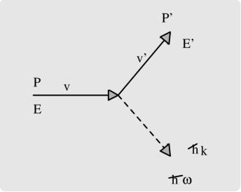
Figure 2: Particle with initial energy $E$ and momentum ${\bf P}$ moving through a transparent medium emits a photon of momentum $\hbar{\bf k}$ and energy $\hbar\omega$ thereby changing its velocity from ${\bf v}$ to ${\bf v}^{\prime}$.

Now substract the formulae for $M^{\prime}$ and $M$ and neglect terms of order higher in ${\cal O}(\omega),{\cal O}({\bf k})$ and ${\cal O}({\bf v^{\prime}}-{\bf v})$:

$$M^{\prime}-M=-\gamma\hbar(\omega-{\bf v}\cdot{\bf k})+\hbar\omega\cdot{\cal O}({\bf v^{\prime}}-{\bf v})$$ (2.1)

The factor ${\cal O}({\bf v^{\prime}}-{\bf v})$ represents recoil effects; it is of order $\hbar\omega/M$ and becomes negligible for a sufficiently heavy particle. In this recoiless limit

$$M^{\prime}-M=-\gamma\hbar(\omega-{\bf v}\cdot{\bf k})$$ (2.2)

Were the particle moving in vacuum, $\,\omega=|{\bf k}|>{\bf v}\cdot{\bf k}$, so that emission would be possible only with de-excitation ($M^{\prime}-M<0$), as plain intuition would have. But in the medium intuition receives a surprise. Let its index of refraction be $n(\omega)>1$. Then $\hbar\omega$ and $\hbar{\bf k}$ are still the energy and momentum of the photon; however $\omega=|{\bf k}|/n(\omega)$. In the case $v\equiv|{\bf v}|>1/n(\omega)$ the particle moves faster than the phase velocity of electromagnetic waves of frequency $\omega$. If $\vartheta$ denotes the angle between ${\bf k}$ and ${\bf v}$, a photon in a mode with $\cos\vartheta>[v\,n(\omega)]^{-1}$ has $\omega-{\bf v}\cdot{\bf k}<0$, and can thus be emitted only in consonance with excitation of the object ($M^{\prime}-M>0$) ! In particular, a particle in its ground state can emit a photon. Ginzburg and Frank [42, 43], who pointed out these phenomena, refer to this eventuality as the anomalous Doppler effect. The reason for the name is that in the case $v<1/n(\omega)$ (subluminal motion for the relevant frequency) when $\omega-{\bf v}\cdot{\bf k}>0$ so that by Eq. (2.1) emission can take place only by de-excitation, the relation between $\omega$ and ${\bf k}$ and the rest frame transition frequency $\omega_{0}\equiv|M-M^{\prime}|/\hbar$, namely

$$\omega_{0}=\gamma(\omega-{\bf v}\cdot{\bf k}),$$ (2.3)

is the standard Doppler shift formula; indeed Ginzburg and Frank refer to this case as the normal Doppler effect. We shall refer to the emission as spontaneous superradiance.

The energy source for superradiant emission and the associated excitation is the bulk motion of the particle. And this emission is not just allowed by the conservation laws; it must occur spontaneously, as follows from thermodynamic reasoning. The particle in its ground state with no photon around constitutes a low entropy state; the excitation of the object to one of a number of possible excited states with emission of a photon with momentum in a variety of possible directions evidently involves an increase in entropy. Thus the emission is favored by the second law of thermodynamics.

The inverse anomalous Doppler effect or superradiant absorption can also take place: when superluminally moving, the particle can absorb a photon only by getting de-excited, and cannot absorb while in the ground state ! The appropriate equation is obtained from Eq. (2.1) by reversing the sign. Obviously superradiance is not restricted to photons. All that is required is that the energy and momentum of a quantum be expressible in terms of frequency and wavevector in the usual way. Thus superradiance can take place for phonons in fluids, plasmons in plasma, etc.

When the particle has no internal degrees of freedom, say a point charge, its rest mass is fixed. We may thus set $M^{\prime}-M=0$ in Eqs. (2.2). The equation cannot then be satisfied for $v<1/n(\omega)$ since its r.h.s. would then be strictly positive: again no absorption or emission is possible from a subluminal particle. However, for $v>1/n(\omega)$ the r.h.s. vanishes for a photon’s whose direction makes an angle $\vartheta$ to the particle’s velocity, where $\cos\vartheta=[v\,n(\omega)]^{-1}$. Such photons must thus be emitted. Obviously as the charge goes by, the front of photons forms a cone with opening angle $2\Theta_{C}=2(\pi/2-\vartheta)$, or $\sin\Theta_{C}(\omega)=[v\,n(\omega)]^{-1}$. This result makes it clear that one is here dealing with the famous Cherenkov radiation, which comes out on just such a cone. Thus Cherenkov radiation is an example of spontaneous superradiance by a structureless charge [43]. Another example [23] is furnished by the Mach shock cone trailing a supersonic object, whose opening angle also corresponds to the condition $\omega-{\bf v}\cdot{\bf k}=0$.

2.2 Superradiant amplification

The above section deals with spontaneous superradiance which occurs when the Ginzburg-Frank condition

$$\omega-{\bf v}\cdot{\bf k}<0$$ (2.4)

is satisfied. I mentioned that the radiation must be emitted in order that the world’s entropy may increase. Einstein’s celebrated argument inextricably connects spontaneous emission with stimulated emission. Therefore, when condition (2.4) is satisfied, there must also occur amplification of preexisting radiation by an object moving superluminally (supersonically) in a medium. Rather than dwell on the simple particle, I shall show this for an object with complicated structure, so that it may dissipate energy internally. The demonstration is thermodynamical (and basically classical). For concreteness I suppose the object to move in a transparent medium filled with electromagnetic radiation.

Let the radiation be exclusively in modes with frequency near $\omega$ and propagating within $\Delta{\bf n}$ of the direction ${\bf n}$. Also let $I(\omega,{\bf n})$ denote the corresponding intensity (per unit area, unit solid angle and unit bandwidth). Experience tells us that the body will absorb power $a(\omega,{\bf n})\,\Sigma({\bf n})\,I(\omega,{\bf n})\,\Delta\omega\Delta{\bf n}$, where $\,\Sigma({\bf n})\,$ is the object’s geometric crossection orthogonal to direction ${\bf n}$, and $a(\omega,{\bf n})<1$ is its absorptivity for the mentioned photons. The remainder power, $[1-a(\omega,{\bf n})]\,\Sigma({\bf n})\,I(\omega,{\bf n})\,\Delta\omega\Delta{\bf n}$, will be scattered. In addition the object may emit spontaneously some power $W$, say by thermal emission. By conservation of energy, absorption and emission cause the object’s total energy (in the laboratory frame) $E$ to change at a rate

$$dE/dt=a\,\Sigma\,I\,\Delta\omega\Delta{\bf n}-W$$ (2.5)

Now the linear momentum conveyed by the radiation is ${\bf k}/\omega$ times the energy conveyed, where ${\bf k}={\bf n}\,\omega n(\omega)$. This is clear if we think of the radiation as composed of quanta, each with energy $\hbar\omega$ and momentum $\hbar{\bf k}$ with $\omega\,n(\omega)=|{\bf k}|$. The result can also be derived from the temporal-spatial and spatial-spatial components of the energy-momentum tensor for the electromagnetic field in a medium. Thus absorption and emission cause the linear momentum ${\bf P}$ of the body to change at a rate

$$d{\bf P}/dt=({\bf k}/\omega)\,a\,\Sigma\,I\,\Delta\omega\Delta{\bf n}-{\bf U}$$ (2.6)

where ${\bf U}$ signifies the rate of spontaneous momentum emission.

In calculating the rate of change of rest mass $M$ of the body, I ignore the effects of elastic scattering because in the frame of the body waves are scattered with no Doppler shift (since there is no motion),so they contain the same energy before and after the scattering. Thus the scattering cannot contribute to $dM/dt$. Obviously the change in $M$ is obtained by a Lorentz transformation:

$$dM/dt=\gamma(dE/dt-{\bf v}\cdot d{\bf P}/dt)$$ (2.7)

Of course, a change in the proper mass means that the number of microstates accessible to the object has changed, i.e., that its entropy $S$ has changed. Recalling the definition of temperature $T=\partial M/\partial S$ and Eqs. (2.5)–(2.6), we see that

$${dS\over dt}=\gamma T^{-1}\,[\omega^{-1}\,(\omega-{\bf v}\cdot{\bf k})\,a\,\Sigma\,I\,\Delta\omega\Delta{\bf n}-W+{\bf v}\cdot{\bf U}\,]$$ (2.8)

The second law does not allow the claim that this last expression is positive because there is also a change in the entropy in the radiation. But one can put an upper bound on the rate of change of the radiation entropy, $d{\cal S}/dt$ by ignoring any entropy carried into the object by the radiation. Now the entropy in a single mode of a field containing on the mean $N$ quanta is at most  [60]

$${\cal S}_{\rm max}=(N+1)\ln(N+1)-N\ln N\approx\ln N$$ (2.9)

where the approximation applies for $N\gg 1$. The scattered waves carry a mean number of quanta proportional to $I(\omega,{\bf n})$. Hence for large $N$ the outgoing radiation’s contribution to $d{\cal S}/dt$ is bounded from above by a quantity of $O[\ln I(\omega,{\bf n})]$. There is an additional contribution of ${\cal O}(W)$ to $d{\cal S}/dt$ coming from the spontaneous emission. Hence

$$d{\cal S}/dt<{\cal O}[\ln I(\omega,{\bf n})]+{\cal O}(W)$$ (2.10)

Because the object dissipates energy, the second law of thermodynamics demands $dS/dt+d{\cal S}/dt>0$. As $I(\omega,{\bf n})$ is made larger and larger, the total entropy rate of change becomes dominated by the term proportional to $I(\omega,{\bf n})$ in Eq. (2.8) because $W$ and ${\bf U}$ are kept fixed. Positivity of $dS/dt+d{\cal S}/dt$ then requires

$$(\omega-{\bf v}\cdot{\bf k})\,a(\omega,{\bf n})>0$$ (2.11)

Thus when the Ginzburg-Frank condition is fulfilled, $a(\omega,{\bf n})<0$. This result was obtained by assuming $a\,\Sigma\,I\,\Delta\omega\Delta{\bf n}\gg W$. But since—barring nonlinear effects—$a$ must be independent of the incident intensity, the result must be true for any intensity which can still be regarded as classical. Now $a<0$ means that the scattered wave, with power proportional to $1-a$, is stronger than the incident one (which is represented by the “1” in the previous expression). Thus the moving object must amplify preexisting radiation in modes satisfying the Ginzburg-Frank condition. Superradiant amplification is mandatory. For modes with $\omega-{\bf v}\cdot{\bf k}>0$, $a>0$ and so the object absorbs on the whole.

Obviously $a$ switches sign at $\omega={\bf v}\cdot{\bf k}$. This switch cannot take place by $a$ having a pole since $a<1$. If $a$ is analytic in $\omega-{\bf v}\cdot{\bf k}$, it must thus have the expansion

$$a\,=\,\alpha({\bf v},{\bf n})\,(\omega-{\bf v}\cdot{\bf k})+\cdots$$ (2.12)

in the vicinity of the superradiant treshold $\omega\,=\,{\bf v}\cdot{\bf k}$. However, we must emphasize that thermodynamics does not require the function $a$ to be continuous at $\omega\,=\,{\bf v}\cdot{\bf k}$.

As an example of both spontaneous superradiance and superradiant amplification we rederive Landau’s critical velocity for superfluidity  [63]. A superfluid can flow through thin channels with no friction. However, when the speed of flow is too large, the superfluidity is destroyed. As Landau did, I phrase the argument in the rest frame of the fluid with respect to which the walls of the channel are in motion. The walls play the role of the object in our superradiance argument, and the waves of frequency $\omega=\varepsilon/\hbar$ and wavenumber ${\bf k}={\bf p}/\hbar$ associated with the quasiparticles in the fluid are surrogates of the electromagnetic waves in both our above arguments. In superfluid He⁴ the dispersion relation $\varepsilon({\bf p})$ has a nonvanishing minimum: $v_{c}\equiv{\rm min}\ \varepsilon({\bf p})/|{\bf p}|>0$.

When the walls move with speed $v>v_{c}$, the quantity $\omega-{\bf v}\cdot{\bf k}=(\varepsilon-{\bf v}\cdot{\bf p})/\hbar\$ becomes negative for at least one quasiparticle mode. According to Sec. 2.1 the wall material will then become excited and simultaneously create quasiparticles in those modes. Furthermore (Sec. 2.2), the quasiparticles thus created can undergo superradiant multiplication while impinging on other parts of the walls. As a consequence, an avalanche of quasiparticle formation ensues, which acts to convert the superfluid into a normal fluid. Thus the transition away from superfluidity is a literal example of the superradiance phenomenon. In this phenomenon the speed $v_{c}$, of order the speed of sound, plays the role of the speed of light in our original arguments.

2.3 Gravitational generation of electromagnetic waves

Now for our first black hole example. Consider an electrically neutral black hole of mass $M$ moving with uniform velocity $\bf v$ through a uniform and isotropic transparent dielectric with index of refraction $n(\omega)$ made of material with atomic mass number $\tilde{A}$ and pervaded by a spectrum of electromagnetic waves. We could be thinking about an astronomical sized black hole moving through a cloud of gas, or about a microscopic black hole whizzing through a solid state detector. Anyway, I assume the hole does not accrete material; however, its gravitational field certainly influences the dielectric.

In applying the argument of Sec. 2.2, the entropy of the object is replaced by the black hole entropy together with entropy of the surrounding dielectric. Now black hole entropy is proportional to the horizon area, and Hawking’s area theorem [46] tells us that black hole area will increase in any classical process, such as absorption of electromagnetic waves by the hole. If the dielectric is ordinary dissipative material, it will also contribute to the increase in entropy through changes it undergoes in the vicinity of the passing hole. Thus an argument like that in in Sec. 2.2 tells us that the black hole plus surrounding dielectric will amplify radiation modes obeying the Ginzburg-Frank condition at the expense of the hole’s kinetic energy. Likewise, even if there are no waves to start with, an argument like that in Sec. 2.1 tells us that the black hole plus dielectric will spontaneusly emit electromagnetic waves in modes that obey the condition.

The process in question is distinct from the standard Cherenkov effect because the hole is neutral. Now waves cannot classically emerge from within the hole, so what is their source ? The hole’s gravity pulls on the positively charged nuclei in the dielectric stronger than on the enveloping electrons. As a result the array of nuclei sags with respect to the electrons, and produces an electrical polarization of the dielectric accompanied by an electric field which ultimately balances the tendency of gravity to rip out nuclei from electrons. It is this electric structure which is to be viewed as the true source of the waves. If one is interested in the intensity of this gravitationally induced electromagnetic radiation, one may map the present problem onto the Cherenkov one by noting that the induced electric field ${\bf E}$ is related to the gravitational one, ${\bf g}$ by $e{\bf E}=-\delta\mu\,{\bf g}$ where $\delta\mu\approx\tilde{A}m_{p}$ is the nuclei-electron mass difference, and $e>0$ the unit of charge. From the gravitational Poisson equation it follows that $\nabla\cdot{\bf E}=4\pi GM(\delta\mu/e)\delta({\bf r}-{\bf r}_{0})$ where ${\bf r}_{0}$ denotes the momentary black hole position. The electric field accompanying the black hole is thus that of a pointlike charge $Q\equiv G\tilde{A}Mm_{p}/e$. This assumes, and this is no trivial assumption [23, 91], that the dielectric has time to relax to allow for the generation of the compensating field. If so, the electromagnetic radiation will be Cherenkov radiation of a charge $Q$ moving with velocity ${\bf v}$. In units of $e$, $Q$ amounts to about $10^{3}\tilde{A}$ times the gravitational radius of the hole measured in units of the classical radius of the electron. Hence a relativistically moving $10^{15}$ g primordial black hole would radiate just like particle with $\sim 10^{3}\tilde{A}$ elementary charges.

2.4 Rotational superradiance

Zel’dovich came upon the notion of black hole superradiance by examining what happens when scalar waves impinge upon a rotating absorbing object  [110]. His later thermodynamic proof [111] that this superradiance is a general feature of rotating objects and any waves provides the inspiration for the argument given in Sec. 2.2. Here I just elaborate on Zel’dovich’s original proof by taking into account the radiation entropy, which he neglected.

I focus on an axisymmetric macroscopic object rotating rigidly in vacuum with constant angular velocity $\Omega$ about a constant axis. Axisymmetry is critical; otherwise precession of the axis would arise. I consider the object to have many internal degrees of freedom, so that it can internally dissipate absorbed energy, and that it rapidly reaches equilibrium with well defined entropy $S$, rest mass $M$ and temperature $T$.

Let the object be exposed to external radiation. By the symmetries we may classify the radiation modes by frequency $\omega$ and azimuthal number $m$. This last refers to the axis of rotation. Suppose that in the modes with azimuthal number $m$ and frequencies in the range in $\{\omega,\omega+\Delta\omega\}$, power $I_{m}(\omega)\,\Delta\omega$ is incident on the body. Then, as is easy to verify from the energy-momentum tensor, or from the quantum picture of radiation, the radiative angular momentum is incident at rate $(m/\omega)I_{m}(\omega)\,\Delta\omega$. If $I_{m}(\omega)$ is large enough, we can think of the radiation as classical. Experience tells us that the body will absorb a fraction $a_{m}(\omega)$ of the incident power and angular momentum flow in the modes in question, where $a_{m}(\omega)<1$ is a characteristic coefficient of the body. A fraction $[1-a_{m}(\omega)\,]$ will be scattered back into modes with the same $\omega$ and $m$. We may thus replace Eqs. (2.5)-(2.6) by

$${dE\over dt} = a_{m}\,I_{m}\,\Delta\omega-W$$ (2.13)

$${dJ\over dt} = (m/\omega)\,a_{m}\,I_{m}\,\Delta\omega-U_{J}$$ (2.14)

where $J$ is the body’s angular momentum and $U_{J}$ is the overall rate of spontaneous angular momentum emission in waves.

Now the energy $\Delta E_{0}$ of a small system measured in a frame rotating with angular frequency ${\bf\Omega}$ is related to its energy $\Delta E$ and angular momentum $\Delta{\bf J}$ in the inertial frame by [59]

$$\Delta E_{0}=\Delta E-{\bf\Omega}\cdot\Delta{\bf J}$$ (2.15)

Thus, when as a result of interaction with the radiation, the energy of our rotating body changes by $dE/dt\times\Delta t$ and its angular momentum in the direction of the rotation axis by $dJ/dt\times\Delta t$, its mass-energy in its rest frame changes by $(dE/dt-\Omega\,dJ/dt)\times\Delta t$. From this we infer, in parallel with the derivation of Eq. (2.8), that the body’s entropy changes at a rate

$${dS\over dt}=T^{-1}\left[\omega^{-1}\,(\omega-m\Omega)\,a_{m}\,I_{m}\,\Delta\omega-W+\Omega\,U_{J}\,\right]$$ (2.16)

As in the discussion involving Eqs. (2.9)-(2.10) we would now argue that when $I_{m}(\omega)$ is large, the term proportional to $(\omega-m\Omega)\,a_{m}(\omega)$ in Eq. (2.16) dominates the overall entropy balance. The second law thus demands that

$$(\omega-m\Omega)\,a_{m}(\omega)>0$$ (2.17)

Thus whenever the condition

$$\omega-m\Omega<0$$ (2.18)

is met, $a_{m}(\omega)<0$ necessarily. As in Sec. 2.2, we can argue that the sign of $a_{m}(\omega)$ should not depend on the strength of the incident radiation if nonlinear radiative effects do not intervene. Hence, independent of the strength of $I_{m}(\omega)$, condition (2.18) is the generic condition for rotational superradiance. It was first found in the context of ordinary objects by Zel’dovich [110].

Evidently $a_{m}(\omega)$ switches sign at $\omega=\Omega m$. This switch cannot take place by $a_{m}(\omega)$ having a pole there since $a_{m}(\omega)<1$. If $a_{m}(\omega)$ is analytic in $\omega-\Omega m$, it must thus have the expansion

$$a_{m}(\omega)=\alpha_{m}(\Omega)\,(\omega-\Omega m)+\cdots$$ (2.19)

in the vicinity of the superradiance treshold $\omega=\Omega m$. However, we must again stress that thermodynamics does not demand continuity of $a_{m}(\omega)$ at $\omega-\Omega m=0$. Specific examples like that of the rotating cylinder  [111, 23] do show continuity.

2.5 Black hole superradiance

By analogy with the results described in Sec. 2.4, Zel’dovich [111] conjectured that a Kerr black hole should also superradiate with respect to modes obeying condition (2.18). This was established directly by Misner [78] for the scalar field case (so that I refer to (2.18) as the Zel’dovich-Misner condition), and some approximate formulae for the gain were worked out by Starobinskii and Churilov [94] (they confirm the rule (2.19)). One can give an illuminating and quick derivation of the necessity for black hole superradiance  [12] starting from Hawking’s area theorem [46]. In the present subsection I take units for which $G=c=1$.

Consider a Kerr black hole of mass $M$ and angular momentum $J$. Its horizon area is

$$A=4\pi\left[\left(M+\sqrt{M^{2}-(J/M)^{2}}\right)^{2}+(J/M)^{2}\right]$$ (2.20)

and small changes of it are given by

$$dA = \Theta_{K}{}^{-1}\cdot\left(dM-\Omega\,dJ\right)$$ (2.21)

$$\Theta_{K} \equiv {\scriptstyle 1\over\scriptstyle 2}A^{-1}\sqrt{M^{2}-(J/M)^{2}}$$ (2.22)

$$\Omega \equiv {J/M\over{r_{\cal H}}^{2}+(J/M)^{2}}$$ (2.23)

Let these changes be caused by absorption from a wavemode whose angular and temporal behavior is ${\cal Y}_{\ell m}(\theta,\phi)e^{-\imath\omega t}\sim{\cal P}(\theta)e^{\imath m\phi-\imath\omega t}$, with ${\cal Y}_{\ell m}$ the spheroidal harmonics (close cousins to the spherical harmonics) relevant to the parameter $J/M$ [94, 99]. As in Sec. 2.4, the overall changes $dM$ and $dJ$ must stand in the ratio $\omega/m$. Thus

$$dM-\Omega\,dJ\propto a_{m}(\omega)(\omega-m\Omega)$$ (2.24)

where $a_{m}(\omega)$ is the absorption coefficient of the black hole and the coefficient of proportionality is positive. Substituting this in Eq. (2.21) and demanding that $dA>0$ tells us that here, as with ordinary rotators, superradiance ensues [$a_{m}(\omega)<0$] when the Zel’dovich-Misner condition holds.

The argument just reviewed differs from that spanning Eqs. (2.13)–(2.18) in that no cognizance need be taken of the radiation entropy. This is because Hawking’s theorem is purely a dynamical one, not a thermodynamic one: classically horizon area increases regardless of what happens to the radiation outside the hole. In particular, one does not have to assume high incident intensity to get the proof to work as was the case for the ordinary rotator. However, suppose the intensity of a superradiant mode illuminating the hole is so low that photons hit it one at a time. Occasionally a photon will tunnel through the potential barrier guarding the black hole and be absorbed. A look at Eqs. (2.21) and (2.18) shows that horizon area will necessarily decrease this time ! Thus this purely quantum process violates Hawking’s area theorem. Now in the framework of semiclassical gravity the only thing that can be going wrong is the theorem’s assumption that the weak energy condition is valid. It apparently is not for a one-photon quantum state.

This immediately opens the door to the Hawking evaporation. For Hawking’s area theorem forbids spontaneous emission from a Kerr black hole only in modes not satisfying the Zel’dovich-Misner condition since such emission would be tantamount to a decrease in horizon area [look at Eq. (2.21)]. The moment the theorem can be sidestepped by quantum processes, spontaneous emission in such modes becomes a possibility. As we know it really happens (Hawking radiance) when the fields are in a particular quantum state (Unruh vacuum). The failure of the area theorem does not destroy the argument for superradiance. One has only to use the argument of Sec. 2.4 with the role of the object’s entropy played by black hole entropy and that of the second law by the generalized second law [9, 13]. One then recovers the proof for superradiance in the Zel’dovich-Misner modes even in the limit of low incident power where one expects that quantum effects foul up the area theorem. We already mentioned that superradiance is a manifestation of stimulated emission. Thus we also expect a corresponding spontaneous emission purely in the superradiant modes. This is Unruh’s nonthermal radiance [101] which emerges from a Kerr black hole, and is distinct from Hawking’s. Unruh’s radiance does not appear in the nonsuperradiant modes.

One other black hole superradiance should be mentioned, namely charge superradiance. Whenever a black hole bears some electric charge and horizon electric potential $\Phi$ (see Eq. (4.27) below), it can superradiate in any mode of a charged bosonic field, e.g. a pion field, which obeys the condition $\omega-(e/\hbar)\Phi<0$, where $e$ denotes the field’s elementary charge. The proof [12] is similar to that for rotational black hole superradiance. Of course, hybrid superradiance involving charged bosons and a Kerr-Newman black hole can also happen. The appropriate Zel’dovich-Misner criterion is left as an exercise to the reader !

2.6 Zel’dovich’s superradiating cylinder

In Sec. 2.4 we saw that the second law of thermodynamics requires that a rotating object superradiate. Now if electromagnetic waves are the issue, how do Maxwell’s equations know that they have to engender superradiance ? This question is analogous to the question how do Einstein’s classical equations know to enforce superradiance as required by the generalized second law of thermodynamics (answer: because they imply the area theorem). In his pioneering paper Zel’dovich [111] remarked that if one is concerned with a steadily rotating weakly conducting cylinder, the electric current induced in it by an incident wave obeying the Zel’dovich-Misner condition has opposite sign to the electric field, so Ohmic dissipation is negative: rather than the wave dissipating, it is enhanced. Zel’dovich’s calculation is skimpy and leaves unanswered the question of how things would work out for large conductivity, or for a dielectric cylinder which dissipates. I concentrate on the dielectric cylinder here; the more general question is dealt with in my paper with Schiffer [23].

I consider a very long dielectric cylinder of radius $R$ made of material with permittivity $\epsilon$ (complex so that the material can dissipate energy) and which rotates steadily with angular frequency $\Omega$. In a dielectric in flat spacetime, Maxwell’s equation take the form

$$F_{[\alpha\beta,\gamma]} = 0$$ (2.25)

$$H^{\alpha\beta}{}_{,\beta} = 0$$ (2.26)

where $H^{\alpha\beta}$ is an antisymmetric tensor built in the style of $F^{\alpha\beta}$, but with the electric displacement ${\bf D}$ replacing ${\bf E}$. Although we shall assume the material is nonmagnetic, the space-space components of $H^{\alpha\beta}$ differ from those of $F^{\alpha\beta}$ unless the medium is stationary. If $u^{\alpha}$ is the medium’s four velocity, the constitutive relations are $H^{\alpha\beta}u_{\beta}=\epsilon F^{\alpha\beta}u_{\beta}$, where $\epsilon$ must be evaluated in the rest frame of the material. A complex relation between field and displacement components is meaningful if we are talking about Fourier components which are complex anyway. I shall assume $\epsilon$ is constant throughout the cylinder.

In ordinary cylindrical coordinates $\{x^{0},x^{1},x^{2},x^{3}\}=\{t,r,\phi,z\}$ we have $u_{\beta}=(-1,0,\Omega r^{2},0)\gamma$ with $\gamma\equiv(1-\Omega^{2}r^{2})^{-1/2}$. The important constitutive relations are

$$H^{31} = F^{31}\equiv B_{\phi}$$

$$H^{23}-\Omega H^{03} = F^{23}-\Omega F^{03}\equiv(r\gamma)^{-1}B_{r}$$ (2.27)

$$(H^{03}-\Omega r^{2}H^{23})\epsilon^{-1} = F^{03}-\Omega r^{2}F^{23}\equiv\gamma^{-1}E_{z}$$

where $E_{z}$, $B_{\phi}$ and $B_{r}$ denote the corresponding physical components of the electric field and magnetic induction in the rotating frame. Relations (2.27) just say that $\epsilon$ is the ratio of electric displacement to electric field in the frame of the dielectric.

Because the rotation is assumed to be a steady one, and there is axisymmetry, one is entitled to write $F^{03}=f(r)e^{\imath(m\phi-\omega t)}$ where $m$ is the azimuthal (integer) quantum number and $\omega$ is the frequency as seen in the stationary frame (I exclude by fiat the possibility of a $z$ variation of the phase). Assuming that all field components behave as $e^{\imath(m\phi-\omega t)}$, I get from Eqs. (2.25–2.26) the components (the rest are not useful for the present discussion)

$$\partial F^{03}/\partial r+\imath\omega F^{31}=0$$

$$\imath\omega F^{23}-\imath mr^{-2}F^{03}=0$$ (2.28)

$$\partial(H^{31}r)/\partial r-\imath mrH^{23}+\imath\omega rH^{03}=0$$

where I have used the flat metric in cylindrical coordinates. The first two equations determine algebraically $F^{31}$ and $F^{23}$ in terms of the complex amplitude $f(r)$. With help of the constitutive relations (2.27) one can eliminate $H^{23}$ and $H^{03}$ from the last equation, being left with

$$r^{2}f^{\prime\prime}+rf^{\prime}-m^{2}f-\left[\omega^{2}+(1-\epsilon)(\omega-m\Omega)^{2}\gamma^{2}\right]r^{2}f=0$$ (2.29)

which is evidently the radial equation for the problem. The fact that the components $F^{12},F^{01}$ and $F^{02}$ do not occur in the system (2.28) means that they can only put in an appearance in a different mode (polarization) with the same $\omega$ and $m$. We can thus set them to zero if we are interested only in the mode governed by $f$.

To determine when superradiance occurs we must have an expression for the radial energy flux. Whether in vacuum or in matter this is given by [61] $S_{r}=({\bf E}\times{\bf H})_{r}/4\pi$ so that here

$$S_{r}=(F^{02}H^{12}-F^{03}H^{31})/4\pi=-F^{03}H^{31}/4\pi$$ (2.30)

This is the instantaneous flux; of more interest is the time averaged flux which can be obtained by first replacing the complex fields by corresponding real expressions [61]

$$F^{03} \rightarrow \left[fe^{\imath(m\phi-\omega t)}+f^{*}e^{-\imath(m\phi-\omega t)}\right]/2$$ (2.31)

$$F^{31} \rightarrow \left[\imath f^{\prime}e^{\imath(m\phi-\omega t)}-\imath f^{*^{\prime}}e^{-\imath(m\phi-\omega t)}\right]/2\omega$$ (2.32)

In the course of time averaging two terms involving exponents $e^{\pm 2\imath(m\phi-\omega t)}$ average out. Using Eqs. (2.27) one gets

$$\overline{S}_{r}=\imath(ff^{*^{\prime}}-f^{*}f^{\prime})/16\pi\omega$$ (2.33)

This expression is clearly real, but its sign is none too clear. To find it out, I calculate with help of the radial equation that

$${d\over dr}[r(ff^{*^{\prime}}-f^{*}f^{\prime})]=2\imath r(\omega-m\Omega)^{2}|f|^{2}\gamma^{2}\Im\epsilon$$ (2.34)

where $\Im$ means “take the imaginary part”. By integrating this equation over $r$ from $r=0$ to $r=R$, and relying on the fact that $\overline{S}_{r}$ must surely be bounded at $r=0$, I get

$$\overline{S}_{r}(r=R)={-1\over 32\pi\omega R}\int_{0}^{R}r(\omega-m\Omega)^{2}|f|^{2}\gamma^{2}\Im\epsilon\,dr$$ (2.35)

By conservation of energy the flux at large distances from the cylinder scales from $\overline{S}_{r}(r=R)$ according to $R/r$ (no sources at $r>R)$.

Now there is a theorem [61] that $\Im\epsilon$ must be an odd function of frequency and positive for positive frequency. This is a requirement of thermodynamic origin. In our case frequency means frequency in the rotating frame. Now the correct azimuthal coordinate in the rotating frame is $\tilde{\phi}=\phi-\Omega t$, so if the phase is to have the form $m\tilde{\phi}-\tilde{\omega}t$, then $\tilde{\omega}$, the frequency as seen in the rotating frame, must be $\omega-m\Omega$. Therefore, the integral above must be negative for $\omega-m\Omega>0$ and positive for $\omega-m\Omega<0$. This means that superradiance (net energy outflux) sets in if and only if the Zel’dovich-Misner condition is satisfied. This is in agreement with the thermodynamic argument of Sec. 2.4, but shows what feature is “microscopically” responsible for the superradiance.

3 Adiabatic invariance

An important turning point in black hole physics occurred with the realization of Christodoulou [35], of Penrose and Floyd [86] and of Hawking [46] that transformations of a black hole generically have an irreversible character. That is, the black hole cannot afterward be brought to its original state. Nowdays we summarize this lore with the rule that horizon area tends to grow, a rule which has gotten identified with the second law of thermodynamics through the correspondence horizon area $\leftrightarrow$ entropy. But equally important is the feature, stressed originally by Christodoulou  [35, 36], that some special processes involving a black hole are truly reversible. These reversible processes give to black hole dynamics a more mechanical flavor than would be the case if horizon area grew under any change of the black hole; they are the analogs of adiabatic changes of a mechanical system. Further details may be found in my contribution to the Festschrifft for Vishveshwara [24] and in the paper by Mayo [74].

In this section I use units with $G=c=1$.

3.1 Adiabatic invariants in general

In mechanics the evolution of a system is dictated by its Hamiltonian $H(q,p)$ (I write only one degree of freedom; there might be many). It may be the case that this Hamiltonian depends on an external parameter $\lambda$: $H(q,p,\lambda)$. For example a charged particle can find itself in an external magnetic field ${\bf B}$ which then plays the role of $\lambda$. Things get interesting when $\lambda=\lambda(t)$ whereupon the Hamiltonian ceases to be conserved. Now suppose the system has a timescale $T$ for a motion which crudely brings it back to the original state or dimensions (quasiperiodic motion). If $\lambda$ changes on a timescale much longer than $T$, the process is called an adiabatic one. Any mechanical quantity, ${\cal A}[q,p]$, which is found to change on a timescale much longer than that of $\lambda$ is called an adiabatic invariant.

Ehrenfest [40] proved that for a system where a particular degree of freedom is separable, the corresponding integral $\oint pdq$ taken around one orbit, usually called an action variable or Jacobi action, is necessarily an adiabatic invariant. Some examples will clarify this. If a particle bounces between two parallel walls whose separation $L(t)$ grows linearly with time, and no forces act on it between bounces, then $\oint pdq=(|p_{\rightarrow}|L_{1}+|p_{\leftarrow}|L_{2})$, where $L_{1}$ is the separation at the end of the rightward motion, etc. This quantity is exactly the same from cycle to cycle (a very good adiabatic invariant). We can say approximately that $\overline{|p(t)|}\propto L(t)^{-1}$, a result of great importance in understanding adiabatic cooling of a gas. If the string of a swinging pendulum of small angular amplitude $\theta$ and frequency $\omega$ is paid out slowly on the timescale $2\pi/\omega$, then $\oint p_{\theta}d\theta\approx 2\pi E/\omega$ with $E$ being a typical value of the total energy in the oscillation. This quantity varies little from one swing to the next, a result which is useful in understanding why photon occupation number is conserved under slow expansion of a radiation filled box. Finally for the charge $e$ moving in a spatially uniform field ${\bf B}(t)$ which varies little in the course of a Larmor orbit, $\oint p_{\varphi}d\varphi\approx 2e\pi BR^{2}$ where $B$ is a typical magnitude of ${\bf B}$ while $R$ is the Larmor radius of the orbit. Again this quantity varies much slower than $B$ from orbit to orbit, allowing us to conclude that the magnetic flux through the orbit is approximately conserved. This result has many implications from plasma physics to astrophysics to condensed matter physics.

The rate of change of a Jacobi action of a system with a smooth Hamiltonian falls off exponentially rapidly as $\dot{\lambda}\rightarrow 0$ [59]. Without smoothness this is not true; for instance, in the example of the particle bouncing between separating walls, if the motion is not linear in time, $\oint pdq$ varies as a low power of $\dot{\lambda}$ as $\dot{\lambda}\rightarrow 0$. And there is nothing in mechanics which forbids adiabatic invariants that are not Jacobi actions. We learn that there may be adiabatic invariants which approach constancy only as power laws in $\dot{\lambda}\rightarrow 0$. In light of this, a useful definition of an adiabatic invariant is that ${\dot{\cal A}/\dot{\lambda}}\rightarrow 0$ as $\dot{\lambda}\rightarrow 0$. This is at variance with the much tighter definition given in mathematically rigorous treatises [3].

Now, does a black hole in near equilibrium have adiabatic invariants, namely quantities which vary very slowly compared to variations of the external perturbations on the black hole ? I will not look for quantities analogous to the Jacobi actions. The Christodoulou reversible processes suggest that horizon area might be an adiabatic invariant. Let us see how with the simplest example.

3.2 Particle absorption by charged black hole

Consider a Reissner-Nordström black hole of mass $M$ and positive charge $Q$. The exterior metric is

$$ds^{2}=-\chi\,dt^{2}+\chi^{-1}\,dr^{2}+r^{2}(d\theta^{2}+\sin^{2}\theta d\varphi^{2}),$$ (3.1)

with

$$\chi\equiv 1-2M/r+Q^{2}/r^{2}.$$ (3.2)

One shoots in radially from far away a classical point particle of mass $m$ and positive charge $\varepsilon$ with total relativistic energy adjusted to the value

$$E=\varepsilon Q/r_{\cal H}.$$ (3.3)

where $r_{\cal H}$ is the $r$ coordinate of the event horizon,

$$r_{\cal H}=M+\sqrt{M^{2}-Q^{2}}$$ (3.4)

In Newtonian terms this particle should marginally reach the horizon where its potential energy just exhausts the total energy. The relativistic equation of motion leads to the same conclusion.

The relativistic action for radial motion is

$$S=\int L\,d\tau=\int{\left[-m\,\sqrt{\chi\,(dt/d\tau)^{2}-(dr/d\tau)^{2}/\chi}-\varepsilon A_{t}\ dt/d\tau\,\right]\,d\tau},$$ (3.5)

where $\tau$, the proper time, acts as a path parameter, and $A_{t}=Q/r\$ is the only nontrivial component of the electromagnetic 4-potential. The stationary character of the background metric and field means that there exists a conserved quantity, namely

$$E=-{\partial L\over\partial(dt/d\tau)}={m\,\chi\over\sqrt{\chi\,(dt/d\tau)^{2}-(dr/d\tau)^{2}/\chi}}\ {dt\over d\tau}+{\varepsilon\,Q\over r}.$$ (3.6)

Since the norm of the 4-velocity is conserved, the square root in this above equation has to be unity. Substituting $dt/d\tau$ from this condition back in Eq. (3.6) gives

$$E=m\,\sqrt{\chi+(dr/d\tau)^{2}}+{\varepsilon\,Q\over r}.$$ (3.7)

It is easy to see that this is precisely the total energy of the particle, for at large distances from the hole, $E\approx m+m\upsilon^{2}/2-m\,M/r+\varepsilon\,Q/r$ (sum of rest, kinetic, gravitational and electrostatic potential energies). Setting $E=\varepsilon\,Q/r_{\cal H}$ shows that the radial motion has a turning point ($dr/d\tau=0$) precisely at the horizon $[\chi(r_{\cal H})=0]$.

Because the particle’s motion has a turning point at the horizon, it gets accreted by it. The area of the horizon is originally

$$A=4\pi{r_{\cal H}}^{2}=4\pi\left(M+\sqrt{M^{2}-Q^{2}}\right)^{2},$$ (3.8)

and the (small) change it incurs upon absorbing the particle is

$$dA=\Theta_{RN}{}^{-1}(dM-Q\,dQ/r_{\cal H})$$ (3.9)

with

$$\Theta_{RN}\equiv{\scriptstyle 1\over\scriptstyle 2}A^{-1}\sqrt{M^{2}-Q^{2}}$$ (3.10)

Thus if the black hole is not extremal so that $\Theta_{RN}\neq 0$, $dA=0$ because $dM=E=\varepsilon Q/r_{\cal H}$ while $dQ=\varepsilon$. Therefore, the horizon area is invariant under the accretion of the particle from a turning point (more precisely, $dA$ is of higher order of smallness than $dM$).

To a momentarily radially stationary local inertial observer, the particle in question hardly moves radially as it is accreted. Thus its assimilation is adiabatic. By contrast, if $E$ were larger than in Eq. (3.3), the particle would not try to turn around at the horizon, and the local observer would see it moving radially at finite speed and being assimilated quickly. And the horizon’s area would increase upon its accretion, as is easy to check from the previous argument. Thus invariance of the horizon area goes hand in hand with adiabatic changes at the black hole, as judged by local observers at the horizon.

The above conclusions fail for the extremal Reissner-Nordström black hole. When $Q=M$, $\sqrt{M^{2}-Q^{2}}$ in Eq. (3.8) is unchanged to ${\cal O}(\varepsilon^{2})$ during the absorption, so that $dA=8\pi ME$. This is not a small change, so the horizon’s area is not an adiabatic invariant. Thus extremal black holes behave differently from generic black holes in this as in other phenomena.

Christodoulou actually first worked out the “reversible process” for a Kerr black hole [35]; that calculation is more complicated than the above. The generalization to the Kerr-Newman black hole was made by Christodoulou and Ruffini [36]. We shall return to it in Sec. 5.

In all the above the particle model of matter is used. What would happen if we let the black hole interact with waves ? One can consider the addition to the black hole of charge by means of a charged wave, and demonstrate the adiabatic invariance of the horizon area under suitable circumstances. The idea will be clear, especially against the background provided by the last paragraph of Sec. 2.5, when we consider the addition of angular momentum to a Kerr black hole via waves.

3.3 Wave absorption by rotating black hole

Consider a Kerr black hole of mass $M$ and angular momentum $J$. Its rotational angular frequency $\Omega$ is given by Eq. (2.23); it is the angular velocity with which every observer near the horizon gets dragged azimuthally. Let distant sources irradiate the black hole with a weak scalar wavemode of frequency $\omega$, “orbital” angular momentum ${\ell}$ and azimuthal “quantum” number $m$. In the spirit of perturbation theory I neglect the gravitational waves so produced. The black hole geometry will eventually be changed by interaction with this wave, but since the latter is taken to be weak, I shall assume that the change amounts to a transition from one Kerr geometry to another with slightly different $M$ and $J$. In the final analysis such assumption is justified by the stability of the Kerr geometry and the no-hair theorems. Since the geometry thus remains axisymmetric and stationary after the change, the wave preserves its angular-temporal form ${\cal Y}_{\ell m}(\theta,\varphi)e^{-\imath\omega t}$ over all time (here ${\cal Y}_{\ell m}(\theta,\varphi)$ denotes a spheroidal harmonic function [94], a cousin of the spherical harmonic $Y_{\ell m}(\theta,\varphi)$).

According to Sec. 2.5 the hole’s absorptivity to scalar waves, $a_{m}(\omega)$, must have the sign of $\omega-m\Omega$: the hole absorbs energy for $\omega-m\Omega>0$ and gives up energy for $\omega-m\Omega<0$. As $\omega\rightarrow m\Omega$, $a_{m}$ must pass through zero because passage through a pole is unthinkable ($a_{m}<1$ always). In fact the general argument leading to Eq. (2.19) is applicable here and tells us that $a_{m}\sim\omega-m\Omega$ near the neutral point. Indeed, Starobinskii and Churilov [94] calculated

$$a_{m}\approx K_{\omega\ell}\cdot\left(\omega-\Omega\,m\right),$$ (3.11)

where $K_{\omega\ell}(M,J)$ is a positive coefficient. It follows from this and by analogy with Eqs. (2.13)-(2.14) that the changes in $M$ and $J$ are

$$dM\propto\omega\left(\omega-\Omega\,m\right)$$ (3.12)

$$dJ\propto m\left(\omega-\Omega\,m\right)$$ (3.13)

with a common positive proportionality constant. By substituting these in Eq. (2.21) we obtain

$$dA\propto\left(\omega-\Omega\,m\right)^{2},$$ (3.14)

again with positive coefficient. The fact that $dA>0$ is in harmony with Hawking’s area theorem [46].

For small $\omega-m\Omega$, say on the scale $M^{-1}$, the long term changes of the system (black hole) are governed by changes in $M$ and $J$ which are seen to be of ${\cal O}(\omega-m\Omega)$. By contrast the horizon area change is of ${\cal O}\big{(}(\omega-m\Omega)^{2}\big{)}$ so that the horizon area behaves like an adiabatic invariant.

In Sec. 3.2 we saw that for the Reissner-Nordström case the process may be termed adiabatic because the particle gets assimilated very slowly by the black hole. For waves in the Kerr case the meaning of “adiabatic” needs to be refined. It is known that a static ($\omega=0$) but nonaxisymmetric perturbation of a Kerr black hole, such as would be caused by field sources held in its vicinity at rest with respect to infinity, necessarily causes an increase in horizon area [48]. However, static perturbations in this sense are not adiabatic from the local point of view. Because of the dragging of inertial frames [77], any nonaxisymmetric static field is perceived by momentarily radially stationary local inertial observers as endowed with temporal variation as these observers are necessarily dragged through the field’s spatial inhomgeneity. At the horizon the dragging frequency is the hole’s rotational frequency $\Omega$, and a field component with azimuthal “quantum” number $m$ is seen to vary with temporal frequency $m\Omega$ which need not be small. Evidently, “adiabatic” must here mean that according to momentarily radially stationary local inertial observers, the perturbation has only low frequency Fourier components. As we saw in Sec. 2.6, the frequency of a wave like ${\cal Y}_{\ell m}(\theta,\varphi)\,e^{-\imath\omega t}\,\propto e^{\imath m\phi-\imath\omega t}$ as sensed by observers rotating with the hole at the horizon is precisely $\omega-m\Omega$, and so it is this frequency which must be small in order for the process to be considered adiabatic. As we just saw, only perturbations with small $\omega-m\Omega$ leave the horizon area invariant to a higher order than other corresponding changes in the black hole.

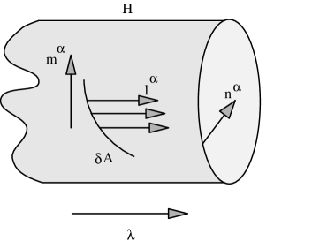
Figure 3: The patch of area $\delta A$ on ${\cal H}$ is formed by null generators whose tangents are $l^{\alpha}=dx^{\alpha}/d\lambda$, where $\lambda$ is an affine parameter along the generators; shown also are the spacelike vector $m^{\alpha}$ and the ingoing null vector $n^{\alpha}$ of the same Newman-Penrose tetrad.

These conclusions are inapplicable to the extremal Kerr black hole ($J=M^{2}$). In this case $\Theta_{K}=0$ (see Sec. 2.5), so one cannot use Eq. (2.21) to calculate the change in area, but must work directly with Eq. (2.20). From Eq. (2.23) one learns that $\Omega=1/2M$ so that $\Delta J=\Omega^{-1}\Delta M=2M\Delta M$. Replacing $M\rightarrow M+\Delta M$ and $J\rightarrow J+2M\Delta M$ in Eq. (2.20), and substracting the original expression gives

$$\Delta A=8\pi(2+\surd 2)M\Delta M+{\cal O}((\Delta M)^{2}).$$ (3.15)

Since a generic addition of mass $\Delta M$ will give a $\Delta A$ of the same order, the horizon area of an extremal Kerr hole is not an adiabatic invariant.

3.4 Dynamics of horizon area

Before delving further into the subject let us review the central result in the field, Hawking’s area theorem [46], and the horizon dynamics upon which it is based.

As usual, we denote the event horizon by ${\cal H}$. Consider a small patch of ${\cal H}$’s area $\delta A$; it is formed by null generators whose tangents are $l^{\alpha}=dx^{\alpha}/d\lambda$, where $\lambda$ is an affine parameter along the generators (see Fig. 3). By definition of the convergence $\rho$ of the generators  [77], $\delta A$ changes at a rate

$$d\delta A/d\lambda=-2\rho\delta A.$$ (3.16)

Now $\rho$ itself changes at a rate given by the optical analogue of the Raychaudhuri equation (with Einstein’s equations already incorporated)  [80, 87]

$$d\rho/d\lambda=\rho^{2}+|\sigma|^{2}+4\pi T_{\alpha\beta}\,l^{\alpha}l^{\beta},$$ (3.17)

where $\sigma$ is the shear of the generators, and $T_{\alpha\beta}$ the energy momentum tensor. The shear evolves according to

$$d\sigma/d\lambda=2\rho\sigma+C_{\alpha\beta\gamma\delta}\,l^{\alpha}m^{\beta}l^{\gamma}m^{\delta},$$ (3.18)

where $C_{\alpha\beta\gamma\delta}$ is the Weyl conformal tensor, and $m^{\alpha}$ one of the spacelike Newman-Penrose tetrad legs which lies in ${\cal H}$.

Many types of classical matter obey the weak energy condition

$$T_{\alpha\beta}\,l^{\alpha}l^{\beta}\geq 0.$$ (3.19)

We have seen in Sec. 2.5 that matter in certain quantum states can violate this condition. In the discussion of adiabatic invariance I take a completely classical view, and will assume that Eq. (3.19) is always true. Then $\rho$ can—according to Eq. (3.17)—only grow or remain unchanged along the generators. Now were $\rho$ to become positive at any event along a generator of our patch, then by Eq. (3.17) it would remain positive henceforth, and indeed grow bigger. Eq. (3.16) then shows that $\delta A$ would shrink to nought in a finite span of $\lambda$ [46, 77] thus implying extinction of generators. But it is an axiom of the subject [46, 77] that ${\cal H}$’s generators cannot end in the future. The only way out is to accept that $\rho\leq 0$ everywhere along the generators, which by Eq. (3.16) signifies that the patch’s area can never decrease. This is the essence of Hawking’s area theorem.

Under what conditions is ${\cal H}$’s area constant ? Hawking [46] and Hawking and Hartle [48] consider this to be possible only if the black hole it exactly stationary. The examples in Secs. 3.2-3.3 show that there are slightly nonstationary situations where the increase in horizon area is imperceptible. Let us characterize the situations where no change in area occurs.

By Eq. (3.16) this requires that $\rho=0$. But then Eq. (3.17) implies that also $\sigma=0$ while $T_{\alpha\beta}\,l^{\alpha}l^{\beta}=0$ on ${\cal H}$. Then Eq. (3.18) implies that $C_{\alpha\beta\gamma\delta}\,l^{\alpha}m^{\beta}l^{\gamma}m^{\delta}$ vanishes on ${\cal H}$. The particular Weyl tensor component in question describes gravitational waves crossing the horizon inward bound. These will not occur if the situation is quasistationary, since gravitational waves are generated by matter only to ${\cal O}(\upsilon^{5})$ where $\upsilon$ is the velocity of the matter sources. Thus as a minimum we must have an approximate time Killing vector and slow motion of matter. This granted, preservation of ${\cal H}$’s area requires in addition

$$T_{\alpha\beta}\,l^{\alpha}l^{\beta}=0\quad{\rm on\ \cal H}.$$ (3.20)

Is this condition always satisfied in a quasistationary situation even when sources of nongravitational fields reside in the vicinity of the black hole ? If not, then there is no hope for an adiabatic theorem because the area will be found to increase even in situations which look like requiring no changes of the black hole.

Computations, some of them arduous, show that the condition indeed holds. It is true for the energy-momentum tensor of either minimally or conformally coupled scalar fields from static sources in a Schwarzschild [24] or Reissner-Nordström [74] black hole’s vicinity, for that from minimally coupled scalar field’s sources axisymmetrically arranged around a Kerr black hole [74], and for the electromagnetic field’s $T_{\mu\nu}$ from charges arranged statically about a Schwarzschild black hole. Energy-momentum conservation is the common reason for the enforcement of Eq. (3.20) in a (nearly) stationary situation. The argument is very simple.

Assume that the exterior geometry has a time translation Killing vector $\xi^{\alpha}$. This might be the only Killing vector as when a Schwarzschild black hole is perturbed by static field sources placed with no particular symmetry around it. Or the situation might also be axisymmetric (additional Killing vector $\eta^{\alpha}$) while still static if the array is made axisymmetric. A third case is that of a nonstatic but still stationary and axisymmetric situation where the black hole rotates with angular frequency $\Omega$. Because ${\cal H}$ is a Killing horizon, the tangent to any of its generators, $l^{\alpha}$, must be along a Killing vector, itself a linear combination of the above Killing vectors. In a truly static situation $l^{\alpha}\propto\xi^{\alpha}$, but if the black hole rotates, $l^{\alpha}\propto(\xi^{\alpha}+\Omega\eta^{\alpha})$. The Killing vector $\zeta^{\alpha}\equiv\xi^{\alpha}+\Omega\eta^{\alpha}$ (with $\Omega\neq 0$ or, if appropriate, $\Omega=0$) defined over all the black hole exterior is an extension of $l^{\alpha}$ off ${\cal H}$. Now because $T^{\alpha\beta}{}_{;\beta}=0$ and $T^{\alpha\beta}=T^{\beta\alpha}$ as well as the Killing equation $\zeta_{\alpha;\beta}+\zeta_{\beta;\alpha}=0$, $(T^{\alpha\beta}\zeta_{\alpha})_{;\beta}=0$. Gauss’s law then gives

$$\int(T^{\alpha\beta}\zeta_{\alpha})_{;\beta}\,(-g)^{1/2}d^{4}x=\oint T^{\alpha\beta}\zeta_{\alpha}\,d\Sigma_{\beta}=0$$ (3.21)

where the second integral is taken over any closed orientable 3-surface, and $d\Sigma_{\beta}$ is the outward pointing element of 3-volume on it.

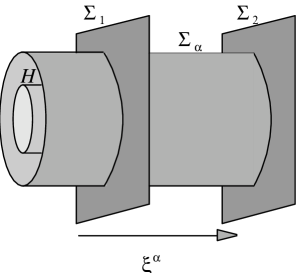
Figure 4: The bounding 3-hypersurface is composed of the section of the horizon $H$ between two constant-time hypersurfaces, $\Sigma_{1}$ and $\Sigma_{2}$, the two hypersurfaces themselves, and the part $\Sigma_{\rm a}$ between $\Sigma_{1}$ and $\Sigma_{2}$ of a spacelike hypersurface in the asymptotically flat region far from the black hole.

As shown in Fig. 4, let us take this 3-surface to be composed of the section of ${\cal H}$ between two constant-time hypersurfaces, $\Sigma_{1}$ and $\Sigma_{2}$, the two hypersurfaces themselves, and the part $\Sigma_{\rm a}$ between $\Sigma_{1}$ and $\Sigma_{2}$ of a spacelike hypersurface with $S^{2}\times R$ topology in the asymptotically flat region far from the black hole. The contribution to the integral from $\Sigma_{2}$ cancels that from $\Sigma_{1}$ because the time translation maps one into the other while leaving $T^{\alpha\beta}$ unchanged, and because the sign of $d\Sigma_{\alpha}$ is opposite on $\Sigma_{1}$ and $\Sigma_{2}$. The $d\Sigma_{\beta}$ on $\Sigma_{\rm a}$ points in the radial direction in suitable coordinates. In the static situation with $\zeta^{\alpha}=\xi^{\alpha}$, $T^{\alpha\beta}\zeta_{\alpha}d\Sigma_{\beta}$ at $\Sigma_{\rm a}$ represent energy flow inward at $\Sigma_{\rm a}$. If no energy influx exists, for example because the ropes supporting various objects that perturb the black hole are not moving, then the contribution of $\Sigma_{\rm a}$ vanishes and we get

$$\int_{\cal H}T^{\alpha\beta}l_{\alpha}d\Sigma_{\beta}=0$$ (3.22)

In the rotating case when $\zeta^{\alpha}\equiv\xi^{\alpha}+\Omega\eta^{\alpha}$, $T^{\alpha\beta}\zeta_{\alpha}\,d\Sigma_{\beta}$ at $\Sigma_{\rm a}$ contains an additional term representing inflow of angular momentum ($T_{r\varphi}\,dt\,r^{2}d\theta\,d\varphi$ in the usual coordinates). In other words, the new term represents a torque on the black hole. If the sources disturbing it are arranged axisymmetrically and coaxially with its rotation, there will be no such torque. In this case we recover Eq. (3.22).

If the weak energy condition (3.19) is satisfied at $\Sigma_{1}$, it is preserved between $\Sigma_{1}$ and $\Sigma_{2}$ by the time translation symmetry. Thus the integral in Eq. (3.22) is a sum of positive semidefinite contributions, one for each horizon patch. Hence Eq. (3.22) implies that Eq. (3.20) is true everywhere on the horizon. There is thus no reason for the area to increase, even secularly. Thus if external sources disturb a Schwarzschild black hole in a static way or a Kerr black hole in a stationary and axisymmetric way, they do not cause the horizon area to grow. This is as we would have liked to believe, but it is reassuring to have a proof that mere presence of matter fields at the horizon does not cause its area to increase. There is thus no impediment of principle to an adiabatic theorem for black holes.

3.5 Black hole disturbed by scalar charges

In Sec. 3.3 I demonstrated the adiabatic invariance of horizon area for a Kerr black hole under the influence of scalar waves. Here I demonstrate the invariance for a Schwarzschild black hole subject to low frequency scalar perturbations originating from sources “rattling” in the hole’s vicinity.

Consider a Schwarzschild black hole with exterior metric

$$ds^{2}=-(1-2M/r)dt^{2}+(1-2M/r)^{-1}dr^{2}+r^{2}(d\theta^{2}+\sin^{2}\theta\,d\varphi^{2}).$$ (3.23)

Suppose sources of a minimally coupled scalar field $\Phi$ have been brought to a finite distance from the hole and are there caused to perform some motion at low frequencies. Does this influence cause an increase in ${\cal H}$’s area ?

If the scalar’s sources are weak, one may regard $\Phi$ as a quantity of first order, and proceed by perturbation theory. The scalar’s energy-momentum tensor,

$$T_{\alpha}{}^{\beta}=\nabla_{\alpha}\Phi\nabla^{\beta}\Phi-{1\over 2}\,\delta^{\beta}_{\alpha}\,\nabla_{\gamma}\Phi\,\nabla^{\gamma}\Phi,$$ (3.24)

will be of second order of smallness. I shall suppose the same is true of the energy-momentum tensor of the sources themselves. Thus to first order the metric (3.23) is unchanged. The scalar equation outside the scalar’s sources can be written

$$-{r^{4}\over(r^{2}-2Mr)}{\partial^{2}\Phi\over\partial t^{2}}+{\partial\over\partial r}\left[(r^{2}-2M){\partial\Phi\over\partial r}\right]-\hat{L}^{2}\,\Phi=0.$$ (3.25)

where $\hat{L}^{2}$ is the usual squared angular momentum operator (but without the $\hbar^{2}$ factor). This equation suggests looking for a solution of the form [77]

$$\Phi=\Re\int_{0}^{\infty}d\omega\sum_{\ell=0}^{\infty}\,\sum_{m=-\ell}^{\ell}C_{\ell m}(\omega)\,f_{\ell m}(\omega,r)\,Y_{\ell m}(\theta,\varphi)e^{-\imath\omega t}.$$ (3.26)

where the $Y_{\ell m}$ are the familiar spherical harmonic (complex) functions. Since the $Y_{\ell m}$ form a complete set in angular space, any function $\Phi(r,\theta,\varphi,t)$ can be so expressed with the help of a Fourier decomposition in the time variable. The constant coefficients $C_{\ell m}(\omega)$ are to be used to match $\Phi$ to the prescribed sources; their presence allows for arbitrary normalization of the $f_{\ell m}$. Since $\hat{L}^{2}Y_{\ell m}=\ell(\ell+1)Y_{\ell m}$, the radial and angular variables separate. In terms of Wheeler’s “tortoise” coordinate $r^{*}\equiv r+2M\ln(r/2M-1)$, for which the horizon resides at $r^{*}=-\infty$, and the new radial function $H_{\ell m}(\omega,r^{*})\equiv rf_{\ell m}(\omega,r)$, one finds for $H_{\ell m}$ the equation

$$-{d^{2}H_{\ell m}\over dr^{*2}}+\left(1-{2M\over r}\right)\left({2M\over r^{3}}+{\ell(\ell+1)\over r^{2}}\right)H_{\ell m}=\omega^{2}H_{\ell m}.$$ (3.27)

Since the index $m$ does not figure here, I write just plain $H_{\ell}(\omega,r)$; one may obviously pick $H_{\ell}$ to be real.

The resemblance between Eq. (3.27) and the Schrödinger eigenvalue equation permits the following analysis [77] of the effects of distant scalar sources on the black hole horizon. Waves with “energy” $\omega^{2}$ on their way in from a distant source run into a positive potential, the product of the two parentheses in Eq. (3.27). The potential’s peak is situated at $r\approx 3M$ for all $\ell$. Its height is $0.0264M^{-2}$ for $\ell=0$, $0.0993M^{-2}$ for $\ell=1$ and $\approx 0.038\,\ell(\ell+1)M^{-2}$ for $\ell\geq 2$. Therefore, waves with any $\ell$ and $\omega<0.163M^{-1}$ coming from sources at $r\gg 3M$ have to tunnel through the potential barrier to get near the horizon. As a consequence, the wave amplitudes that penetrate to the horizon are small fractions of the initial amplitudes, most of the waves being reflected back. In fact, the tunnelling coefficient vanishes in the limit $\omega\rightarrow 0$ [77]. This means that adiabatic perturbations by distant sources (which surely means they only contain Fourier components with $\omega\ll M^{-1}$) perturb the horizon very weakly (this is just the inverse of Price’s theorem [77] that a totally collapsed star’s asymptotic geometry preserves no memories of the star’s shape). Thus one would not expect significant growth of horizon area from adiabatic scalar perturbations originating in distant sources.

What if the scalar’s sources are moved into the region $2M<r<3M$ inside the barrier ? They will now be able to perturb the horizon; do they change it’s area ? To check let us look for the solutions of Eq. (3.27) in the region near the horizon where the potential is small compared to $\omega^{2}$; according to the theory of linear second order differential equations they are of the form

$$H_{\ell\omega}(r^{*})=\exp(\pm\imath\omega r^{*})\times[1+{\cal O}(1-2m/r)].$$ (3.28)

The Matzner boundary condition [71] that the physical solution be an ingoing wave, as appropriate to the absorbing character of the horizon, selects the sign in the exponent as negative. Hence the typical term in $\Phi$ is

$${1+{\cal O}(1-2m/r)\over r}P_{\ell}(\cos\theta)\,\cos\psi;\qquad\psi\equiv\omega(r^{*}+t)-m\varphi.$$ (3.29)

We obviously require that the event horizon remain regular under the scalar’s perturbation; otherwise the black hole would be destroyed. A minimal requirement for regularity is that physical invariants like $\Upsilon_{1}\equiv T_{\alpha}{}^{\alpha}$, $\Upsilon_{2}\equiv T_{\alpha}{}^{\beta}T_{\beta}{}^{\alpha}$, $\Upsilon_{3}\equiv T_{\alpha}{}^{\beta}T_{\beta}{}^{\gamma}T_{\gamma}{}^{\alpha}$, etc., be bounded, for divergence of any of them would surely induce curvature singularities via the Einstein equations. By Eq. (3.24) the invariant $\Upsilon_{k}$ is always proportional to $(\Phi_{,\alpha}\Phi^{,\alpha})^{k}$. For a single mode like that in Eq. (3.29), an explicit calculation on the Schwarzschild background using $dr^{*}/dr=(1-2M/r)^{-1}$ gives, after a miraculous cancellation of terms divergent at the horizon (pointed out by A. Mayo),

$$\Phi_{,\alpha}\Phi^{,\alpha}\propto{m^{2}P_{\ell}{}^{2}\sin^{2}\psi\over r^{4}\sin^{2}\theta}+\left({dP_{\ell}\over d\theta}\right)^{2}{\cos^{2}\psi\over r^{4}}+{\omega\sin(2\psi)\over r^{3}}P_{\ell}^{2}+\cdots\,,$$ (3.30)

where “$\ \cdots\$” here and henceforth denote terms that vanish as $r\rightarrow 2M$. This expression is bounded at the horizon. Now suppose $\Phi$ is the sum of two modes like (3.29), which we label with subscripts “1” and “2”. Then a calculation gives $\Phi_{,\alpha}\Phi^{,\alpha}$ as consisting of three groups of terms, two of them of form (3.30) with subscripts 1 and 2, respectively, and a third of the form

$${m_{1}m_{2}P_{\ell_{1}}P_{\ell_{2}}\sin\psi_{1}\sin\psi_{2}\over r^{4}\sin^{2}\theta}+\left({dP_{\ell_{1}}\over d\theta}\right)\left({dP_{\ell_{2}}\over d\theta}\right){\cos\psi_{1}\cos\psi_{2}\over r^{4}}+$$

$$+{\omega_{1}\sin\psi_{1}\cos\psi_{2}+\omega_{2}\sin\psi_{2}\cos\psi_{1}\over r^{3}}P_{\ell_{1}}P_{\ell_{2}}+\cdots$$ (3.31)

This is also bounded. By induction any $\Phi$ of form (3.26) will give a bounded $\Phi_{,\alpha}\Phi^{,\alpha}$. Thus all the $\Upsilon_{k}$ are bounded at $r=2M$, and a generic scalar perturbation does not disturb the horizon unduly.

The extent to which the black hole is perturbed must be linear in the magnitude of the invariant $\Upsilon_{1}$ (Einstein’s equations have $T_{\alpha\beta}$ as source, not $T_{\alpha}{}^{\gamma}T_{\gamma}{}^{\beta}$). It is then clear from both our results that this perturbation is of order ${\cal O}(\omega^{0})$ generically, and of ${\cal O}(\omega)$ in the monopole case. As we shall now see, the change in the horizon area is of ${\cal O}(\omega^{2})$, so that for small $\omega$ the area is (relatively) invariant.

A 3-D hypersurface of the form $\{\forall t,r={\rm const.}\}$ has as tangent the Killing vector $\xi^{\alpha}=\delta_{t}{}^{\alpha}$ with norm $-(1-2M/r)$, and as normal $\eta_{\alpha}=\partial_{\alpha}(r-{\rm const.})=\delta_{\alpha}{}^{r}$ with norm $(1-2M/r)$. The vector $N^{\alpha}\equiv\xi^{\alpha}+(1-2M/r)\eta^{\alpha}$ is obviously null, and as $r\rightarrow 2M$ both its covariant and contravariant forms remain well defined, so that it must there be proportional (with finite nonvanishing proportionality constant) to $l^{\alpha}$, the tangent to the horizon generator. This can be verified by remarking that $N^{\alpha}$, just as $l^{\alpha}$, is null, future pointing ($N^{t}>0$) as well as outgoing ($N^{r}>0$).

Now

$$T_{\alpha\beta}N^{\alpha}N^{\beta}=(T_{r}{}^{r}-T_{t}{}^{r})\,N_{r}\,N^{r}+2T_{t}{}^{r}N_{r}N^{t}.$$ (3.32)

From $N^{\alpha}$’s definition we have $N_{r}N^{r}=1-2M/r$ and $N_{r}N^{t}=1$. And from Eq. (3.24) it is clear that $T_{r}{}^{r}-T_{t}{}^{t}=\Phi_{,r}\Phi^{,r}-\Phi_{,t}\Phi^{,t}$ while $T_{t}{}^{r}=\Phi_{,t}\Phi^{,r}$. Thus

$$T_{\alpha\beta}N^{\alpha}N^{\beta}=[\Phi,_{t}+(1-2M/r)\Phi,_{r}]^{2}.$$ (3.33)

If one now substitutes a $\Phi$ made up of a single mode like in Eq. (3.29), one concludes that

$$T_{\alpha\beta}l^{\alpha}l^{\beta}\propto{\omega^{2}P_{\ell}^{2}\sin^{2}\psi\over r^{2}}+\cdots\,.$$ (3.34)

A quick way to this result is to recognize that $l^{\alpha}\propto\xi^{\alpha}\equiv(\partial/\partial t)^{\alpha}$ because the horizon generators must lie along the only Killing vector field of the problem. In view of Eq. (3.24) and the null character of $l^{\alpha}$,

$$T_{\alpha\beta}l^{\alpha}l^{\beta}\propto(\Phi,_{\alpha}\xi^{\alpha})^{2}=(\partial\Phi/\partial t)^{2},$$ (3.35)

which reproduces Eq. (3.34). And if one substitutes the generic $\Phi$, the proportionality to the square of frequency will obviously remain.

Thus, when scalar field sources are moved inside the barrier, they perturb the geometry by an amount which does not, in general, vanish as the perturbations is made to change slower and slower. By contrast, the rate of change of the horizon area vanishes as the square of the typical Fourier frequency of the perturbation. In this sense the horizon area is an adiabatic invariant. The result has been generalized by Mayo [74] for electromagnetic fields from charges near a Schwarzschild black hole. That calculation was harder than the one above, and succeeded only by judicious use of the analogy between electrodynamics in a curved spacetime and in a flat spacetime filled with a medium with appropriately varying permittivity and permeability [104].

3.6 Sketch of a proof of the adiabatic theorem

The above permits us to discuss a process quite different from those treated in Secs. 3.2–3.3. In those cases the black hole is transformed by the process, its charge or angular momentum changing, so that the adiabatic process converts one Kerr-Newman black hole into another. But imagine instead slowly bringing a scalar charge from a distance to near a Schwarzschild’s black hole horizon, and then withdrawing it slowly as well. The horizon undergoes a perturbation which is then relaxed. According to Sec. 3.5, the horizon’s area does not change appreciably, so the black hole must return to its original Schwarzschild state. We now sketch a simple proof of the adiabatic theorem for the same kind of situation, but for any sort of matter perturbations, which need not be small.

We assume a static black hole is surrounded by charges of some sort which perturb it via their fields; these charges are assumed supported in some way, for example by ropes coming down from large distances. The black hole need not be close to Schwarzschild; it could be strongly distorted from sphericity. This, of course, does not violate the no-hair principle because the black hole is not an isolated black hole.

Now suppose the charges, initially at rest, are set into slow motion, for instance by being lowered slowly with help of the ropes. Let $\upsilon$ be the signed scale of the velocity involved. For example, this could be the typical proper radial velocity of one of the charges. The sign of $\upsilon$ distinguishes one slow motion from its exact reversal, all starting from the same configuration.

Let $\xi^{\alpha}$ be the Killing vector of the background geometry before motion sets in and let $T^{\alpha}{}_{\beta}$ denote the exact energy-momentum tensor, at all times, of the sources and their fields. The spacelike components of $T^{\alpha}{}_{\beta}\,\xi^{\beta}$, the energy flux components defined with respect to the background metric, $g^{(0)}_{\mu\nu}$, obviously switch sign together with $\upsilon$. If we assume that $T^{\alpha}{}_{\beta}\,\xi^{\beta}$ can be expanded in a series in $\upsilon$, that series must thus start with ${\cal O}(\upsilon)$. By the Einstein equations linearized about $g^{(0)}_{\mu\nu}$, some of the components of the metric perturbations coming from the motion, $\delta g_{\mu\nu}$, must be of ${\cal O}(\upsilon)$. This means that the black hole is generically distorted to ${\cal O}(\upsilon)$. However, it does not follow that the horizon’s area changes to ${\cal O}(\upsilon)$.

We saw in Sec. 3.4 that for a static situation $\rho=\sigma=C_{\alpha\beta\gamma\delta}\,l^{\alpha}m^{\beta}l^{\gamma}m^{\delta}=0$; thus $g^{(0)}_{\mu\nu}$ by itself must give $\rho=\sigma=C_{\alpha\beta\gamma\delta}\,l^{\alpha}m^{\beta}l^{\gamma}m^{\delta}=0$ while $\delta g_{\mu\nu}$ [which has some components of ${\cal O}(\upsilon)$] will generate corrections $\delta\rho$, $\delta\sigma$ and $\delta(C_{\alpha\beta\gamma\delta}\,l^{\alpha}m^{\beta}l^{\gamma}m^{\delta})$ of ${\cal O}(\upsilon)$ or higher. Now look at Eqs. (3.18). Its right hand side is of ${\cal O}(\upsilon)$ so $d\delta\sigma/d\lambda={\cal O}(\upsilon)$. This is consistent with $\delta\sigma$ being of ${\cal O}(\upsilon)$ because $\delta\sigma\rightarrow 0$ in the far future when things settle down to staticity.

Eq. (3.17) now tells us that the question of whether $d\delta\rho/d\lambda$ is of ${\cal O}(\upsilon)$ or ${\cal O}(\upsilon^{2})$ is determined by the order of $T_{\alpha\beta}l^{\alpha}l^{\beta}$, the other terms in the right hand side being necessarily of ${\cal O}(\upsilon^{2})$. We showed in Sec. 3.4 that $T_{\alpha\beta}l^{\alpha}l^{\beta}=0$ for the background situation involving no motion. Can $T_{\alpha\beta}l^{\alpha}l^{\beta}$ be of ${\cal O}(\upsilon)$ for the dynamic situation in question ? No ! That eventuality would allow it to switch sign with $\upsilon$, but this would contravene the weak energy condition Eq. (3.19). We conclude that $T_{\alpha\beta}l^{\alpha}l^{\beta}={\cal O}(\upsilon^{2})$, or higher. Then Eq. (3.17), together with the requirement that $\delta\rho\rightarrow 0$ in the future when all changes die out, tells us that $\delta\rho={\cal O}(\upsilon^{2})$. It finally follows from Eq. (3.16) that the overall change in horizon area is of ${\cal O}(\upsilon^{2})$. This shows that the change in horizon area is of higher order of smallness than those of the changes undergone by the perturbation of the hole; but this is precisely what the adiabatic theorem would claim.

4 Black hole quantization

Quantum gravity effects supposedly become important only at the Planck scale, variously stated as ${\cal M}_{P}=(\hbar/G)^{1/2}\approx 1.2\times 10^{20}\,{\rm MeV}$ or ${\cal L}_{P}=(\hbar G)^{1/2}\approx 1.6\times 10^{-33}\,{\rm cm}$. Now this scale is so extreme by laboratory standards that it would seem one shall never be able to put quantum gravity to the test in the laboratory. Is this really so or is it possible that by some recondite effect quantum gravity may make itself felt well below the Planck energy (well above the Planck length) ? The Hawking radiance, it is true, is expected also well away from the Planck scale. However, it is generally acknowledged that derivations of it (at least those not based on superstring theory) are semiclassical in nature (no quantum gravity), and cannot tell us what would really happen at the Planck scale. In this lecture I show how one can use a mixture of classical hints and quantum ideas to guess what the departure from Hawking’s simple spectrum should be. The surprise is that there are serious departures expected well away from the Planck regime.

I stated the basic idea [15] immediately after the appearance of the Hawking radiance paper. It was taken up later by Mukhanov [79], and we eventually synthesized our ideas [19, 22]. Other references are my Marcel Grossman VIII talk [25] and my talk at the XVII Brazilian Meeting on Particles and Fields [20].

Henceforth in this section I use units with $G=c=1$ and denote the charge of the electron by $-e$.

4.1 Quantum numbers of a black hole

In setting out to give a quantum description of black holes, a primary question (first asked by Wheeler in the late 1960’s) is what is the complete set of quantum numbers required to describe a black hole in a stationary quantum state. Quantum numbers are first and foremost attributes of elementary particles. Now an elementary object with mass below ${\cal M}_{P}$ has its gravitational radius tucked below its Compton wavelength; it is thus properly termed “elementary particle”. By contrast an elementary object with mass above ${\cal M}_{P}$ has its Compton wavelength submerged under the gravitational radius; it is best called a black hole. The discontinuity between the two occasioned by the emergence of the horizon is illusory because at the Planck scale the spacetime geometry should be quite fuzzy. So there is no in between regime here, and by continuity the smallest black holes should be quite like elementary particles, and should merit description by a few quantum numbers like mass, charge, spin, etc.

As the black hole gets larger, it should become more classical and thus come into the province of Wheeler’s no-hair principle (see Secs. 1.1-1.2): a black hole is parametrized only by mass, spin angular momentum, electric and magnetic charge. Of course there are the nonabelian generalizations of the Kerr-Newman solutions. But as we saw, with the exception of the Skyrmionic black hole, these are all unstable. I now argue, by analogy with field theory, that we need not promote the parameters of these unstable solutions to the status of quantum numbers.

Recall the Higgs field with Mexican hat potential in flat spacetime. A homogeneous configuration of Higgs field taking on a value on the slope of the potential is not a stationary classical solution. No stationary quantum state corresponds to it. A configuration with the field at a minimum of the potential is a classical stationary stable solution. Small perturbations away from it, which classically oscillate around it, are interpreted in the quantum theory as excitations of the field above the minimum state. By contrast, a configuration with the field at a maximum of the potential is a classical stationary but unstable solution. A small perturbations away from it runs away. In the quantum theory such perturbations are reinterpreted as tachyonic excitations. To us this really means that the underlying stationary configuration are pathological.

By analogy we may conclude that to each stable stationary classical black hole solution corresponds a stationary quantum state which is capable of excitation. Again by analogy, the excited state can be interpreted as the base black hole state plus quanta of various fields propagating on its background. By contrast, an unstable stationary classical black hole solution cannot be associated with a stationary quantum state because excitations of the later would be tachyonic in nature. Thus, the unstable nonabelian hair black holes and the BBM black hole do not furnish classical analogues of quantum stationary states.

Of course the above argument cannot rule out quantum stationary black hole states without classical analogs. But it does suggest that, as far as present evidence requires, the only quantum numbers of a stationary black hole state are mass, spin angular momentum, electric and magnetic charge and Skyrmionic topological number. As mentioned in Sec. 1.2, this last is a kind of winding number, and as such not obviously additive. For this reason I strike it from the list.

4.2 Mass spectrum of a black hole

I thus focus on black hole eigenstates of the operators mass $\hat{M}$, angular momentum $\hat{\bf J}^{2}$ and $\hat{J}_{z}$, electric charge $\hat{Q}$, magnetic charge $\hat{\cal G}$ and, of course, linear momentum ${\hat{\bf P}}$. This last can be set to zero if we agree to work in the black hole’s center of mass. The eigenvalues of $\hat{Q},\hat{\cal G},\hat{\bf J}^{2},{\hat{J}}_{z}$ are well known. By making the standard assumption that these operators are mutually commuting, we may immediately establish the spectrum of the mass for the extremal black holes [75].

The classical extremal Kerr-Newman black hole is defined by the vanishing of the square root in the expression for the Boyer-Lindquist radius of the horizon:

$$r_{\cal H}=M+\sqrt{M^{2}-Q^{2}-{\cal G}^{2}-{\bf J}^{2}/M^{2}}$$ (4.1)

This means

$$M^{2}=Q^{2}+{\cal G}^{2}+{\bf J}^{2}/M^{2}$$ (4.2)

Now solve for $M$ and discard the negative root solution (it gives imaginary $M$). One enforces the quantization of charge, magnetic charge and spin angular momentum by replacing in this expression $Q\rightarrow qe$, ${\cal G}\rightarrow g\hbar/2e$ and $J^{2}\rightarrow j(j+1)\hbar^{2}$ with $q,g$ integers and $j$ a nonnegative integer or half-integer. One thus obtains the mass eigenvalues first found by Mazur [75]

$$M_{qgj} = {\cal M}_{P}\left[\beta_{qg}+\sqrt{\beta_{qg}^{2}+j(j+1)}\right]^{1/2}$$ (4.3)

$$\beta_{qg} \equiv q^{2}e^{2}/2\hbar+g^{2}\hbar/8e^{2}$$ (4.4)

What the above manipulations really mean is the following. The classical constraint (4.2) is replaced by the quantum statement

$$(\hat{M}^{2}-\hat{Q}^{2}-\hat{\cal G}^{2}-\hat{\bf J}^{2}/\hat{M}^{2})\,|qgj\rangle=0$$ (4.5)

which picks out the extreme black hole states $\,|qgj\rangle$ whose mass eigenvalues are given by Eq. (4.3). Any black hole state not anhilated by the shown operator is just not the quantum analog of an extreme black hole. For the moment I sidestep the question of factor ordering ($\hat{M}^{2}$ and $\hat{\bf J}^{2}$ may not commute).

For nonextremal black holes one does not have a constraint like Eq. (4.2). One can, however, proceed from the Christodoulou-Ruffini formula for the mass of the Kerr-Newman black hole in terms of its area (irreducible squared mass): [36]

$$M^{2}={A\over 16\pi}\left(1+{4\pi(Q^{2}+{\cal G}^{2})\over A}\right)^{2}+{4\pi{\bf J}^{2}\over A}$$ (4.6)

This can be obtained by substituting Eq. (4.1) into the generalization of Eqs. (2.20) and (3.8), namely

$$A=4\pi(r_{\cal H}{}^{2}+{\bf J}^{2}/M^{2}),$$ (4.7)

and solving for $M^{2}$. One should note that only the parameter domain

$$A^{2}\geq 16\pi^{2}[(Q^{2}+{\cal G}^{2})^{2}+4{\bf J}^{2}]$$ (4.8)

of Eq. (4.6) is physical. For smaller $A$ the Ruffini-Christodoulou formula has $M^{2}$ decreasing with increasing $A$ (for fixed $Q$, ${\cal G}$ and ${\bf J}^{2}$), a trend which contradicts Eq. (4.7) with Eq. (4.1) substituted in. Obviously when restriction (4.8) does not hold, formula (4.6) is an extraneous root.

In converting Eq. (4.6) to a quantum relation between the operators $\hat{M}$, $\hat{Q}$, $\hat{\cal G}$ and $\hat{\bf J}$, one faces the problem of factor ordering. Now the area of a black hole should be invariant under rotations of its spin; since ${\bf\hat{J}}$ is the generator of such rotations, one sees that $[\hat{A},\hat{\bf J}]=0$. Similarly, area should remain invariant under gauge transformation whose generator is, as usual, the charge $\hat{Q}$. Hence $[\hat{A},\hat{Q}]=0$. Duality invariance of the Einstein-Maxwell equations would then suggest that $[\hat{A},\hat{\cal G}]=0$. Hence one may merely replace the parameters in Eq. (4.6) by the corresponding operators:

$$\hat{M}^{2}=\left[{\hat{A}\over 16\pi}\left(1+{4\pi(\hat{Q}^{2}+\hat{\cal G}^{2})\over\hat{A}}\right)^{2}+{4\pi\hat{\bf J}^{2}\over\hat{A}}\right]\Theta\left(\hat{A}^{2}-16\pi^{2}[(\hat{Q}^{2}+\hat{\cal G}^{2})^{2}+4\hat{\bf J}^{2}]\right)$$ (4.9)

The Heavyside $\Theta$ (step) function enforces the physical restriction Eq. (4.8); when this last is violated, a zero mass eigenvalue is predicted, which means there is no such black hole. One may thus read off the mass eigenvalues of the Kerr-Newman black hole; this approach was first used in Ref. [15].

Two comments are in order. One might object that it is not obvious that the operators $\hat{A}$, $\hat{M}$, $\hat{Q}$, $\hat{\cal G}$ and $\hat{\bf J}^{2}$ are related in exactly the same way as the classical quantities. Might not the classical relation (4.6) arise as an expectation value of some more complicated looking quantum relation ? This is possible, but the available evidence does not seem to require any such complication. If one can neglect fluctuations of the various observables, the expectation value of formula (4.9) will reproduce the Christodoulou-Ruffini formula. The second comment is that it seems nothing was gained in putting (4.9) forward. To judge from the classical situation, $\hat{A}$ would seem to have a continuous spectrum, and so all that (4.9) tells us is that there are several continuum mass sectors, one for each set of eigenvalues of {$\hat{Q},\hat{\cal G},\hat{\bf J}^{2}\}$. The next section shows the evidence pointing to a discrete spectrum for $\hat{A}$.

4.3 Discrete spectrum for horizon area

As we saw in Sec. 3, the horizon’s area of a nonextremal black hole is an analog of an adiabatic invariant in mechanics. This is interesting to us because one can often understand classical adiabatic invariance in simple quantum terms. As an example consider the plain harmonic oscillator. When it is in a stationary state (labeled by quantum number $n$), $E/\omega=(n+{\scriptstyle 1\over\scriptstyle 2})\hbar$. One expects $n$ to remain constant during an adiabatic change (changing the spring constant or the length of a pendulum) because the perturbations imposed on the system have frequencies $\ll\omega$, so that by perturbation theory, quantum transitions between states of different $n$ are strongly suppressed. Therefore, the ratio $E/\omega$ should be preserved. Now for the harmonic oscillator the Jacobi action is $\oint p\,dq=2\pi E/\omega$ so it should be preserved. Thus a quantum insight here gives us an easy understanding of the classical adiabatic invariance of the Jacobi action involved.

Ehrenfest generalized this insight into a principle [40]: any classical adiabatic invariant (action integral or not) corresponds to a quantum entity with discrete spectrum. Again, the rationale is that an adiabatic change, by virtue of its slowness, is expected to lead only to continuous changes in the system, not to jumps that change a discrete quantum number. The preservation of the value of the quantum entity then explains the classical invariance. Ehrenfest’s idea was embodied in the Bohr-Wilson-Sommerfeld quantization rules of the old quantum theory:

$$\,\oint p\,dq=2\pi\hbar n$$ (4.10)

Ehrenfest’s hypothesis can be used profitably in many problems. A not too well known example concerns a relativistic particle of rest mass $m$ and charge $e$ spiralling in a magnetic field ${\bf B}$. One knows that the Larmor spiralling frequency is

$$\Omega={e|{\bf B}|\over\gamma m}={e|{\bf B}|\over E}$$ (4.11)

where $\gamma$ is Lorentz’s factor $(1-\upsilon^{2})^{-1/2}$, and $E$ the total energy. When ${\bf B}$ varies (in space or in time) slowly over one Larmor radius $r$ or over one Larmor period $2\pi/\Omega$, there exists, by Ehrenfest’s theorem, an adiabatic invariant of the form

$$\oint p\,dq=\,\oint m\gamma\Omega r\,d\ell=2\pi e|{\bf B}|r^{2}=2e\varphi,$$ (4.12)

namely, the magnetic flux $\varphi$ through one loop of orbit [53]. Now rewrite the energy

$$E=m\left(1-\dot{r}^{2}-\dot{z}^{2}-r^{2}\Omega^{2}\right)^{-1/2}$$ (4.13)

by replacing $\dot{z}\rightarrow p_{z}/m\gamma$, taking into account that $\dot{r}$ is nearly vanishing, and replacing $\Omega$ and $r^{2}$ by means of Eq. (4.11) and Eq. (4.12) to get

$$E^{2}=m^{2}+p_{z}^{2}+e^{2}r^{2}B^{2}=m^{2}+p_{z}^{2}+e^{2}\varphi B/\pi$$ (4.14)

By Ehrenfest’s principle, in the quantum problem $\varphi$ should have a discrete spectrum. One is thus led to expect that for fixed $p_{z}$, $E^{2}$ should be quantized, possibly with uniformly spaced eigenvalues. And indeed, the exact solution of the relativistic Landau problem with the Klein-Gordon equation [64] leads to the spectrum

$$E^{2}=m^{2}+p_{z}^{2}+e\hbar B(2n+1);\qquad n=0,1,\cdots$$ (4.15)

which justifies the prediction from the Ehrenfest principle.

I now take seriously the analogy between horizon area and adiabatic invariants to conjecture, in harmony with Ehrenfest’s principle, that the area of an equilibrium black hole has a discrete spectrum. We do not have any evidence that one can express horizon area in the form $\oint p\,dq$. Therefore, one should not immediately jump to the conclusion that the area eigenvalues are equally spaced. After all, what if horizon area corresponded to $(\oint p\,dq)^{2}$ rather than to $\oint p\,dq$ ? Thus at first I only write the area eigenvalues as

$$a_{n}=f(n);\qquad n=1,2,3,\cdots$$ (4.16)

The function $f$ must clearly be positive and monotonically increasing (this last just reflects the ordering of eigenvalues by magnitude). In light of Eq. (4.9) and the quantization of charge, magnetic charge, and angular momentum, this conjecture implies that the nonextremal Kerr-Newman black hole also has a discrete mass spectrum. Its form will be elucidated in Sec. 4.5.

How are the area eigenvalues really spaced ? One can obtain a hint by elaborating on Christodoulou’s reversible processes, a special case of which (for a Reissner-Nordström black hole) was discussed Sec. 3.2. More generally Christodoulou and Ruffini [36] showed that the assimilation of a point classical particle by a Kerr-Newman black hole can be made reversibly if the particle, which may be electrically charged and carry angular momentum, is injected at the horizon from a radial turning point in its orbit. In this case the horizon area (or equivalently the irreducible mass) is left unchanged, so that the effects on the black hole can be undone by a second reversible process which adds charges and angular momentum opposite in sign to those added by the first. One can check that Christodoulou and Ruffini’s calculation establishes reversibility only for nonextremal black holes.

4.4 Quantum Christodoulou processes

In the Christodoulou-Ruffini process the particle follows a bound classical orbit, and must be a point particle in order for its absorption to leave the area unchanged. Particularly the first requirement clashes with quantum theory. The particle cannot both be at the horizon and be at a turning point; this contradicts the uncertainty principle because “turning point” means the radial momentum is exactly zero and this is incompatible with being precisely “at the horizon”. How then do we formulate the Christodoulou-Ruffini process while taking cognizance of quantum mechanics for the particle ?

The first thing to settle is the condition under which one can work with classical bound orbits at all. According to the tenets of quantum mechanics this requires that the particle be in a state with large quantum number. Thus let us imagine a particle of mass $\mu<{\cal M}_{P}$ and charge $e$ in a quantum stationary state in the spherically symmetric field of a Reissner-Nordström black hole with mass $M\gg{\cal M}_{P}$ and charge $Q<M$. In this preliminary investigation we ignore relativistic effects, and focus on Schrödinger’s problem in the attractive potential $V=(-M\mu+Qe)/r$ (hence $M\mu>Qe$). The radii of Bohr orbits of order $n$ are [76]

$$R_{n}={n^{2}\hbar^{2}\over\mu(M\mu-Qe)}$$ (4.17)

We require $R_{n}\approx M$ for a fairly large $n$ so that only semiclassical states are involved in describing the particle near the black hole. Thus

$${\hbar\over\mu M}\ll\left(1-{eQ\over\mu M}\right)^{1/2}$$ (4.18)

An additional requirement is that the particle’s Compton length $\hbar/\mu$ be much smaller than $r_{\cal H}\sim M$, so that one can speak of the particle localized near ${\cal H}$. For $Qe$ not approximately equal to $\mu M$, the second requirement guarantees that restriction (4.18) is satisfied; for $Qe\approx\mu M$, restriction (4.18) already takes care of making the Compton length small on scale $M$. In any case, consideration of semiclassical orbits near ${\cal H}$ requires $\hbar/(\mu M)\ll 1$.

We now turn to the general relativistic problem. We generalize the black hole to a Kerr-Newman one (mass $M$, charge $Q$ and spin parameter $a\equiv J/M$). Boyer-Lindquist coordinates $r$ and $\theta$ are used; the following abbreviations are useful:

$$\Delta \equiv r^{2}-2Mr+a^{2}+Q^{2}$$ (4.19)

$$\rho^{2} \equiv r^{2}+a^{2}\cos^{2}\theta$$ (4.20)

It may be noted that $\Delta=0$ at ${\cal H}$.

The condition $\hbar/(\mu M)\ll 1$ granted, we should be able to describe the motion of the particle away from a turning point by applying WKB approximation [76] to a wave packet representing the particle. This means the packet’s center of mass will move classically on a geodesic or—if the particle is charged—on the appropriate solution of the Lorentz equation in Kerr-Newman spacetime. At the turning point the WKB approximation breaks down [76], so we expect the above description to fail. However, since the gist of the quantum description is the existence of uncertainty relations, it should be possible to obtain correct relations between the various parameters of the orbit if we replace the physical radial momentum at the turning point by the radial momentum uncertainty $\delta P$, and the proper radial distance of the turning point from the horizon by the radial proper distance uncertainty $\hbar/\delta P$. This has to be done in the integrated classical orbits.

Carter [32] was first to find the first integrals for the meridional ($\theta$) and radial ($r$) motions in the Kerr-Newman background. The first integrals can be combined as in Misner, Thorne and Wheeler [77]:

$$0 = \tilde{\alpha}E^{2}-2\tilde{\beta}E+\tilde{\gamma}$$ (4.21)

$$\tilde{\alpha} \equiv (r^{2}+a^{2})^{2}-a^{2}\sin^{2}\theta\Delta$$ (4.22)

$$\tilde{\beta} \equiv (r^{2}+a^{2})(aL_{z}+eQr)-aL_{z}\Delta$$ (4.23)

$$\tilde{\gamma} \equiv (aL_{z}+eQr)^{2}-(L_{z}^{2}/\sin^{2}\theta+\mu^{2}\rho^{2})\Delta-\rho^{4}\left[(p^{r})^{2}+(p^{\theta})^{2}\Delta\right]$$ (4.24)

Here $E$ and $L_{z}$ denote the total energy and angular momentum about the symmetry axis of the particle, while $p^{r}$ and $p^{\theta}$ denote the appropriate contravariant momentum components. It proves useful to express these last in terms of the physical components (in an orthonormal tetrad) $P\equiv\Delta^{-1/2}\rho\,p^{r}$ and $\Pi\equiv\rho\,p^{\theta}$. Note that $\Pi$ bears dimension of a linear momentum.

Following Christodoulou and Ruffini (see also Appendix A in Ref. [13]), one solves the quadratic for $E$ taking care to select the root which would give positive energy far from the hole. We are only interested in the expression near the horizon where $\Delta$ is small, so one may replace $r\rightarrow r_{\cal H}$ and $\rho^{2}\rightarrow\rho_{\cal H}{}^{2}$ everywhere except in $\Delta$ itself. Pulling a factor $\Delta$ out of the root we get after some rearrangement

$$E-\Omega L_{z}-e\Phi = {\Delta^{1/2}\over r_{\cal H}{}^{2}+a^{2}}\sqrt{{B^{2}\over\sin^{2}\theta}+\rho_{\cal H}{}^{2}(\mu^{2}+P^{2}+\Pi^{2})}+{\cal O}(\Delta^{3/2})$$ (4.25)

$$\Omega \equiv a(r_{\cal H}{}^{2}+a^{2})^{-1}\rightarrow{\rm rotational\ angular\ frequency}$$ (4.26)

$$\Phi \equiv Q\,r_{\cal H}(r_{\cal H}{}^{2}+a^{2})^{-1}\rightarrow{\rm electrical\ potential}$$ (4.27)

$$B \equiv L_{z}-\Omega(aL_{z}+r_{\cal H}\,Qe)\sin^{2}\theta$$ (4.28)

$\Omega$ is identified with the angular frequency of the hole because it turns out to coincide with the dragging angular frequency at the horizon [77]. Likewise $\Phi$ is interpreted as the hole’s electrical potential because it equals the component $A_{t}$ of the vector potential evaluated at ${\cal H}$.

As mentioned, one may not set $\Delta=0$ in Eq. (4.25) even if one is interested in capture by the black hole because of the uncertainty principle. It thus pays to reexpress the prefactor of the square root in Eq. (4.25) in terms of the (small) proper radial distance $\ell$ of $r$ from $r_{\cal H}$. One easily calculates that

$$\ell\equiv\int_{r_{\cal H}}^{r}\sqrt{g_{rr}}\,dr\approx{2\rho_{\cal H}(r-r_{\cal H})^{1/2}\over(r_{\cal H}-r_{\cal C})^{1/2}}\approx{2\rho_{\cal H}\Delta^{1/2}\over(r_{\cal H}-r_{\cal C})}$$ (4.29)

where $r_{\cal C}$ is the radius of the inner (Cauchy) horizon [negative square root in Eq. (4.1)]. We may thus rewrite Eq. (4.25) as

$$E-\Omega L_{z}-e\Phi={(r_{\cal H}-r_{\cal C})\ell\over 2\rho_{\cal H}(r_{\cal H}{}^{2}+a^{2})}\sqrt{{B^{2}\over\sin^{2}\theta}+\rho_{\cal H}{}^{2}(\mu^{2}+P^{2}+\Pi^{2})}$$ (4.30)

Let us now calculate the change in horizon area occasioned by the particle’s capture. The differential of Eq. (4.7) is

$$dA = \Theta_{KN}^{-1}(dM-\Omega dJ-\Phi dQ)$$ (4.31)

$$\Theta_{KN} \equiv (r_{\cal H}{}^{2}+a^{2})^{-1}(r_{\cal H}-r_{\cal C})/16\pi$$ (4.32)

Not coincidentally, $\Omega$ and $\Phi$ appear here. Their physical identifications are again clear from analogy with thermodynamic formulae. We must of course substitute $dM=E$, $dQ=e$ and $dJ=L_{z}$ in accordance with energy, charge and angular momentum conservation. In view of the result (4.30) we have

$$dA=8\pi\ell\sqrt{{B^{2}\over\rho_{\cal H}{}^{2}\sin^{2}\theta}+\mu^{2}+P^{2}+\Pi^{2}}$$ (4.33)

In this equation $\theta$ represent the meridional angle at which the capture takes place while $\ell$ is a measure of the radial proper distance from the horizon at which the particle can be said to merge with the black hole. In the classical case the limit $\ell\rightarrow 0$ recovers for us Christodoulou’s reversible process for the nonextremal black holes (the turning point condition is $p^{r}\rightarrow 0$ or $\ell P\rightarrow 0$). But $dA$ cannot be zero in the quantum case. We are interested in the minimum possible value for $dA$ required by quantum mechanics. Actually quantum mechanics places no onerous limits on $\Pi$; since we are not terribly interested on precisely where on the horizon the particle hits, one can tolerate substantial uncertainty in angle $\theta$, or equivalently in the linear coordinate $r_{\cal H}\theta$. As its canonically conjugate momentum, $\Pi$ is allowed to have a small uncertainty. More precisely, we could have $\Pi\sim\delta\Pi\sim\hbar/r_{\cal H}$ so that the contribution to $dA$ is $\sim\hbar(\ell/r_{\cal H})$. Of course our whole treatment presupposes that the particle can approach the horizon close compared to the latter’s radius, so the contribution to $dA$ can be made negligible compared to $\hbar={\cal L}_{P}{}^{2}$.

Now the sign of $L_{z}$, the angular momentum along the symmetry axis, is free. One can classically arrange for $L_{z}$ to be such as to nullify the quantity $B$. In the quantum theory $L_{z}$, is quantized, as usual, with the spectrum (no spin) $\hbar\times\{\cdots\,-2,-1,0,1,2,\,\cdots\}$. But this occasions no special problem. Suppose first that $Qe=0$. Then we can certainly pick $L_{z}=0$ so that $B$ makes no contribution to $dA$. Now suppose $Qe$ is nonzero. Our whole treatment presupposes that absorption of the particle is a small perturbation on the hole, so that $|e|\ll|Q|$. Since charge is quantized in of $\approx(\hbar/137)^{1/2}$ we see that $|eQ|\gg\hbar/137$. Now for the Kerr-Newman black hole $\Omega r_{\cal H}\leq 1/2$ and $\Omega a\leq 1/2$. Thus unless the black hole is nearly nonrotating, it is possible to select a nonzero eigenvalue of $L_{z}$ which nullifies $B$ with an error no larger than about $\hbar$. For a hole very close to nonrotating or an accretion point near the hole’s pole (so that $|a\Omega eQ|\sin^{2}\theta<\hbar$), this can be accomplished with $L_{z}=0$. Hence the term $B^{2}$ under the root in Eq. (4.33) contributes to $dA$ at most a term of ${\cal O}(\hbar\ell/\rho_{\cal H})$. Again the contribution to $dA$ can be made small compared to ${\cal L}_{P}{}^{2}$.

The contribution to $dA$ of the $P^{2}$ term under the square root cannot be made so small. At the turning point $P$ cannot be said to vanish, but must be replaced by its uncertainty $\delta P$. And the center of the particle cannot be placed at the horizon with accuracy better than the radial position uncertainty $\hbar/\delta P$; thus $\ell^{2}P^{2}>\hbar^{2}$. Likewise, the particle cannot be localized to better than a Compton wavelength $\hbar/\mu$ so that $\ell^{2}\mu^{2}>\hbar^{2}$. It follows that there must exist a quantum lower bound on $dA$:

$$(dA)_{\rm min}=8\pi\xi\hbar=\alpha\,{\cal L}_{P}{}^{2}$$ (4.34)

where the numerical coefficient $\xi$ takes into account the inherent fuziness of the uncertainty relation. Incidentally, this conclusion fails for extremal black holes because $\Theta_{KN}$ in Eq. (4.31) diverges in that case. The minimal increase in area is then not Eq. (4.34), but a quantity dependent on $M$, $Q$ and $J$, just as in the example discussed at the end of Sec. 3.2. But, surprisingly, for nonextremal black holes $(dA)_{\rm min}$ turns out to be independent of the black hole parameters $M$, $Q$ and $J$.

It is in order to emphasize the approximations made in obtaining Eq. (4.34). We assumed the particle only slightly perturbs the black hole. Thus if it is charged, $Q\gg(\hbar/137)^{1/2}$ and in any case $M\gg\mu$. We also assumed the particle can get close to the horizon which means $M\gg\ell>\hbar/\mu$. Of course, the last two inequalities are consistent by our original assumption that $M\gg\surd\hbar={\cal M}_{P}$.

4.5 Spacing and multiplicity of the area eigenvalues

The fact that, as soon as one allows quantum nuances to the problem, there is, for nonextremal black holes, a minimum horizon area increase suggests that this $(dA)_{\rm min}$ corresponds to the spacing between eigenvalues of $\hat{A}$ in the quantum theory. And the fact that $(dA)_{\rm min}$ is a universal constant suggests that the spacing between eigenvalues is a uniform spacing. For it would be strange indeed if that spacing were to vary, say, as mass of the black hole, and yet the increment in area resulting from the best approximation to a reversible process would contrive to come out universal, as in Eq. (4.34), by involving a number of quantum steps inversely proportional to the eigenvalue spacing. I thus conclude that for nonextremal black holes the spectrum of $\hat{A}$ is

$$a_{n}=\alpha\,{\cal L}_{P}{}^{2}\,(n+\eta);\quad\ \eta>-1;\quad n=1,2,\cdots$$ (4.35)

where the condition on $\eta$ excludes nonpositive area eigenvalues. Since Eq. (4.34) fails for an extremal Kerr-Newman black hole, one cannot deduce as above that its area eigenvalues are evenly spaced. This is entirely consistent with Eq. (4.3) according to which the area spectrum is then very complicated.

For nonextremal black holes the evidence of Sec. 4.4 only suggests a uniformly spaced spectrum well above the Planck scale. Thus Eq. (4.35) is supported for large $n$, or for any $n$ if $\eta\gg 1$. However, I shall go beyond the concrete evidence and assume that the formula is valid also at low quantum numbers even if $\eta={\cal O}(1)$. Some support for this comes from the heuristic picture of a patchwork horizon discussed below.

Thus far I have said nothing about entropy; the discussion has been at the level of mechanics, not statistical physics. But Eq. (4.35) allows us to understand, in a pleasant and intuitive way, the mysterious proportionality between black hole entropy and horizon area.

The quantization of horizon area in equal steps brings to mind an horizon formed by patches of equal area $\alpha\,{\cal L}_{P}{}^{2}$ which get added one at a time. There is no need to think of a specific shape or localization of these patches. It is their standard size which is important, and which makes them all equivalent. This patchwork horizon can be regarded as having many degrees of freedom, one for each patch. After all, the concept “degree of freedom” emerges for systems whose parts can act independently, and here the patches can be added to the patchwork one at a time. In quantum theory degrees of freedom independently manifest distinct states. Since the patches are all equivalent, each will have the same number of quantum states, say, $k$. Therefore, the total number of quantum states of the horizon is

$$N=k^{A/(\alpha{\cal L}_{P}{}^{2})}$$ (4.36)

where $k$ is a positive integer and the effects of the $\eta$ zero point in Eq. (4.35) are glossed over in this, heuristic, argument.

The $N$ states may not all be equally probable. But if the $k$ states of each patch are all equally likely, then all $N$ states are equally probable. In that case the statistical (Boltzmann) entropy associated with the horizon is $\ln N$ or

$$S_{BH}={\ln k\over\alpha}{A\over{\cal L}_{P}{}^{2}}$$ (4.37)

Thus is the proportionality between black hole entropy and horizon area justified in simple terms. Even if not all $k$ states are equally probable, one can still use Eq. (4.37) provided $k$ is regarded as an effective number of equally probable states. Only at this point thus one compare Eq. (4.37) with Hawking’s formula for $S_{BH}$ to calibrate the constant $\alpha$:

$$\alpha=4\ln k$$ (4.38)

The above argument depends crucially on the uniformly spaced area spectrum. The logic leading to the number of states Eq. (4.36) was used in the early days of black hole thermodynamics by me [10] and by Sorkin [93] without regard to any particular area spectrum, but these early arguments are not really convincing because their partition of the horizon into equal area cells would be without basis if the desired result, entropy $\propto$ area, were not known.

Mukhanov’s [79, 19] alternate route to Eqs. (4.36) and (4.38) starts from the accepted formula relating black hole area and entropy. In the spirit of the Boltzmann-Einstein formula, he views $\exp(S_{BH})$ as the degeneracy of the particular area eigenvalue because $\exp(S_{BH})$ quantifies the number of microstates of the black hole that correspond to a particular macrostate (a black hole with definite $M$, $Q$ and ${\bf J}$). Since black hole entropy is determined by thermodynamic arguments only up to an additive constant, one writes, in this approach, $S_{BH}=A/4{\cal L}_{P}{}^{2}+$ const. Substitution of the area eigenvalues from Eq. (4.35) gives the degeneracy corresponding to the $n$-th area eigenvalue:

$$g_{n}=\exp\left({a_{n}\over 4{\cal L}_{P}{}^{2}}+{\rm const.}\right)=g_{1}\ e^{\alpha(n-1)/4}$$ (4.39)

As stressed by Mukhanov, since $g_{n}$ has to be integer for every $n$, this is only possible when [19, 22]

$$g_{1}=1,2,\cdots\quad{\rm and}\quad\alpha=4\times\left\{\ln 2,\ln 3,\cdots\right\}$$ (4.40)

The simplest option would seem to be $g_{1}=1$ (nondegenerate black hole ground state). Here the additive constant in Eq. (4.39) must be negative: were it zero, the area $a_{1}$ would also vanish which seems an odd thing for a black hole. Just this case was studied in Ref. [19]; it is a bit ugly in that the eigenvalue law Eq. (4.35) and the black hole entropy include related but undetermined additive constants.

The next simplest case, $g_{1}=2$ (doubly degenerate black hole ground state), no longer requires the ugly additive constant in the black hole entropy to keep $a_{1}$ from vanishing. With this constant set to zero and the choice $\alpha=4\ln 2$ corresponding to $k=2$, Eqs. (4.35) and (4.39) require that $\eta=0$ so that one is rid of the second ugly constant as well. The area spectrum is

$$a_{n}=4{\cal L}_{P}{}^{2}\ln 2\cdot n;\quad n=1,2,\cdots$$ (4.41)

’t Hooft has independently found evidence for a fundamental unit of area on the horizon of size $4{\cal L}_{P}{}^{2}\ln 2$ [100].

Spectrum (4.41), which I shall adopt henceforth, is good for nonextremal Kerr-Newman black holes. The corresponding degeneracy of area eigenvalues

$$g_{n}=2^{n}$$ (4.42)

corresponds to a doubling of the degeneracy as one passes from one area eigenvalue to the next largest. Mukhanov [79] thought of this multiplicity as the number of ways in which a black hole in the $n$-th area level can be made by first making a black hole in the ground state, and then proceeding to “excite it” up the ladder of area levels in all possible ways. Danielsson and Schiffer [37] considered this multiplicity as representing rather the number of ways the black hole with area $a_{n}$ can “decay” down the staircase of levels to the ground state. In either case there are $2^{n-1}$ ways. The extra factor of two in the scheme here adopted comes from the double degeneracy of the ground state.

To what extent do these intuitively physical predictions correspond to results from more formal quantum gravity schemes ? Mention should be made of Kogan’s string theoretic argument [56], and the quantum membrane approaches of Maggiore [67] and Lousto [66] which establish the uniformly spaced area eigenstates as the base for excitations of the black hole. The efforts of D-brane aficionados (for a review see Ref. [84]) have rather concentrated on the question of degeneracy qua entropy, and it is not clear that they have anything to say about a discrete mass spectrum.

There are also several canonical quantum gravity treatments of a shell or ball of dust collapsing on its way to black hole formation. Those by Schiffer [92] and Peleg [85] obtain a uniformly spaced area spectrum. But Berezin [26], as well as Dolgov and Khriplovich [38], obtain mass spectra for the ensuing black hole which correspond to discrete area spectra with nonuniform spacing (and in Berezin’s approach the levels are infinitely degenerate). Other canonical quantum gravity approaches by Louko and Mäkelä [65], Barvinskii and Kunstatter [8], Mäkelä [68] and Kastrup [54] treat rather a spherically symmetric vacuum spacetime that gets endowed with dynamics by some subtlety; they also come up with a uniformly spaced area spectrum. There is, however, no general agreement on the spacing of the levels. The analogous treatment of the charged black hole by Mäkelä and Repo [70] gets a nonuniform area spectrum.

In the loop quantum gravity approach (for a review see Ref. [4]) the black hole area spectrum is discrete but with a spacing which narrows with increasing area, becoming virtually continuous in the infinite area limit. This is completely at variance with the uniformly spaced spectrum. However, as noticed by I. Khriplovich [55], the area spectrum for the extremal neutral Kerr black hole according to Mazur [Eq. (4.3] coincides in part with the loop gravity horizon area spectrum.

The contradictory conclusions mentioned support the view that none of the existing formal schemes of quantum gravity is as yet a quantum theory of gravity. Clearly a role exists for the heuristic approach.

5 Black hole spectroscopy

Of the ramifications of the discrete area spectrum, the most surprising is the prediction of quasidiscrete spectral lines from a black hole, even one well away from the Planck scale. In this last lecture I explore this aspect. I continue to use units with $G=c=1$.

5.1 The mass levels and a paradox

In the operator relation (4.9) we substitute the area spectrum (4.41). The mass eigenvalues of the Kerr-Newman black hole are thus [15]

$$M_{nqgj} = {\cal M}_{P}\left[{n\ln 2\over 4\pi}\left(1+{2\pi\beta_{qg}\over n\ln 2}\right)^{2}+{\pi j(j+1)\over n\ln 2}\right]^{1/2}$$ (5.1)

$$n > {2\pi\over\ln 2}\sqrt{\beta_{qg}^{2}+j(j+1)}$$ (5.2)

where $\beta_{qg}$ is the same as in Eq. (4.4) and the constraint on $n$ comes from the Heavyside function in Eq. (4.9); we have written a strict inequality because we know that formula (5.1) applies to nonextremal black holes only.

For zero charges and spin the mass spectrum is of the form

$$M\propto\surd n;\qquad n=1,2,\,\cdots$$ (5.3)

implying the $n\Longrightarrow n-1$ transition frequency

$$\omega_{0}\equiv dM/\hbar=(8\pi M)^{-1}\ln 2$$ (5.4)

This simple result is in agreement with Bohr’s correspondence principle: “transition frequencies at large quantum numbers should equal classical oscillation frequencies”, because a classical Schwarzschild black hole displays ‘ringing frequencies’ which scale as $M^{-1}$, just as Eq. (5.4) would predict. This agreement would be destroyed if the area eigenvalues were unevenly spaced. Indeed, the loop gravity spectrum mentioned in Sec. 4.5 fails this correspondence principle test (practitioners of loop gravity are content with trying to recover the Hawking semiclassical spectrum in some limit—see review in Ref. [4].

It follows from the discussion in Sec. 4.4 that absorption of a massive particle by the hole always causes a jump in black hole mass of at least $dM$ (this corresponds to $dA=4{\cal L}_{P}\ln 2$). What if the particle is very light ($\mu\ll\hbar/M$), or if we replace it by a photon ($\mu=0$). The discussion in Sec. 4.4 is no longer relevant since we cannot follow the localized particle to near the horizon: we have to treat the particle as a wave. Then a paradox—the treshold paradox—arises. Scatter off a Schwarzschild black hole an electromagnetic wave whose frequency $\omega$ is below $\omega_{0}$, or is not a precise multiple of $\omega_{0}$. Photons in the wave do not have the right frequency to cause a transition between two mass levels. It would seem that none of the wave can be absorbed. Admittedly, the transmissivity is small at small frequencies, but the quantum prediction of no absorption contrasts starkly with the classical picture of some absorption. And when $\omega\gg\omega_{0}$, the classical transmission coefficient for electromagnetic waves is close to unity, so one sees no correspondence between the quantum picture espoused here and the accepted classical picture, even in the limit of large black holes. Does all this mean the area spacing we have postulated is not really there ?

One should not confuse the question of the classical transmissivity with the question of quantum absorptivity. The transmissivity is determined by the potential barrier around the black hole that shows up in the electromagnetic wave equation. By contrast, the statement that a photon cannot get absorbed unless its frequency is $\omega_{0}$ or a multiple thereof is a quantum gravity statement. A single photon with $\omega<\omega_{0}$ should never be absorbed (modulus the question of line broadening and splitting to be discussed below) even though it has some probability of penetrating the potential barrier [94]. But if we are dealing with a macroscopic wave with $\omega<\omega_{0}$, multiple photon absorption may help to achieve the treshold; re-emission of photons with frequency $\neq\omega$ is then possible. This would be analogous to multiphoton processes in nonlinear optical media where the incident frequencies are shifted. This anomalous absorption would be interpreted in classical theory as the expected absorption of subtreshold frequencies. Now consider a photon with $\omega=100.3\,\omega_{0}$. It also is not in resonance with the black hole levels. But after negotiating the potential barrier, which it does easily because of its high frequency [94], it may get absorbed with re-emission of a quantum with frequency $0.3\,\omega_{0}$, or $1.3\,\omega_{0}$, etc. One would thus expect that a macroscopic wave with $\omega=100.3\,\omega_{0}$ can get partially absorbed with accompanying re-emission of lower frequency radiation.

Admittedly this absorbing behavior of black holes is at variance with what one is accustomed to expect from quantum field theory on a fixed background, where a wave’s frequency is not shifted while scattering off a stationary object. But such shifts are seen in nonlinear optics, and gravitation is a nonlinear phenomenon.

5.2 The black hole line emission spectrum

By analogy with atomic transitions, a black hole at some particular mass level would be expected to make a transition to some lower level with emission of one or more quanta of any of the fields in nature. In the sequel I call these photons for short. The corresponding line spectrum—very different from the Hawking semiclassical continuum—was first discussed in Ref. [15] and further analyzed much later [19, 22]. According to Eq. (5.4) the spacing between mass levels is uniform over a small range of $M$. Thus quantum jumps larger than the minimal produce emission at all frequencies which are integral multiples of $\omega_{0}$: $\omega=\omega_{0}\,\delta n$ with $\delta n=1,2,\,\cdots\,$.

As Mukhanov was first to remark [19, 22], this simple spectrum provides a way to make quantum gravity effects detectable even for black holes well above the Planck mass: the uniform frequency spacing of the black hole lines occurs at all mass scales, and the unit of spacing is inversely proportional to the black hole mass over all scales. Of course, for very massive black holes, one would expect all the lines to become dim and unobservable (just as in the semiclassical description the Hawking radiance intensity goes down as $1/M^{2}$), but there should be a mass regime (primordial mini-black holes ?) well above Planck’s for which the first few uniformly spaced lines should be detectable under optimum circumstances. It is thus important to understand clearly the nature of the line spectrum.

First we must know the ratio of line intensities. Again proceeding by analogy with the perturbation theory of atomic line transitions, each line intensity should be proportional to the square of a matrix element, to the photon energy $\hbar\omega_{0}\delta n$, to the photon phase space factor, and to the degeneracy of the final black hole state. We do not know anything about the matrix element, or even what the relevant operator is. Thus it seems wisest to assume that the matrix element does not vary much as one goes from a nearest neighbor transition (frequency $\omega=\omega_{0}$) to one between somewhat farther neighbors ($\omega=\omega_{0}\,\delta n$). Thus, aside from the question of normalization of the spectrum, the matrix element does not enter into our simple estimate.

The phase space factor is, as usual, $\omega^{2}=(\omega_{0}\,\delta n)^{2}$. The final black hole state’s degeneracy factor is $2^{n-\delta n}$ where $n$ refers to the initial state. Thus all possible transitions from the state $n$ will give lines with frequencies $\omega=\omega_{0}\,\delta n$ and intensities proportional to $(\omega_{0}\delta n)^{3}\exp(-\delta n\ln 2)=\omega^{3}\exp(-\delta n\ln 2)$. The same result can be had by relying on the relation between the Einstein coefficient of spontaneous emission $A_{\downarrow}$ and that for absorption $B_{\uparrow}$ (this last equivalent to the squared matrix element):

$$A_{\downarrow}=B_{\uparrow}{\hbar\omega^{3}\over 4\pi^{2}}{g_{\rm down}\over g_{\rm up}}=B_{\uparrow}{\hbar\omega^{3}\over 4\pi^{2}}{2^{n-\delta n}\over 2^{n}}$$ (5.5)

With $\omega\rightarrow\omega_{0}\,\delta n$ this gives the same result stated earlier. Therefore, the line spectrum emitted by the black hole is expected to be

$$I(\omega)\propto\sum_{\delta n=1}^{\infty}\Gamma(\omega)\,\hbar\omega^{3}\exp(-\omega\ln 2/\omega_{0})\,\delta(\omega-\omega_{0}\,\delta n)$$ (5.6)

where $\Gamma(\omega)$ is the transmission coefficient through the potential barrier surrounding the black hole averaged over angular momenta of the quanta.

This result should be compared with Hawking’s semiclassical spectrum

$$I(\omega)\propto{\Gamma(\omega)\hbar\omega^{3}\over\exp(\hbar\omega/T_{\rm BH})-1}={\Gamma(\omega)\hbar\omega^{3}\over\exp(\omega\ln 2/\omega_{0})-1}$$ (5.7)

where we have used Eq. (5.4) and the standard expression for the Hawking temperature $T_{\rm H}=\hbar/8\pi M$. It may be seen that, apart from the question of normalization, Hawking’s spectrum becomes the envelope of the line spectrum for $\omega\gg\omega_{0}$ while “overshooting” slightly the first few lines. Both the existence of lines and the “deficiency” in the first few as compared to the thermal spectrum are predictions of the heuristc approach.

The above is not to say that the emission spectrum should be a pure line spectrum. Multiple photon emission in one transition will also contribute a continuum. To go back to atomic analogies, the transition from the 2s to the 1s states of atomic hydrogen, being absolutely forbidden by one-photon emission, occurs with the long lifetime of 8 s by two-photon emission (photon splitting in the jargon). The hydrogenic spectrum is thus a continuum over the relevant frequency range. We have already mentioned multiphoton absorption as a possible resolution of the “treshold paradox”. By detailed balance some multiple photon emission should accompany decay of the black hole from higher to lower mass levels which should generate a continuum that would compete with the line spectrum [19, 22]. However, for the black hole no reason is known why one-photon transition would be forbidden. Thus my expectation, again based on the atomic analogy, is that most of the energy will get radiated in one-photon transitions which give lines. The spectrum, in first approximation, should be made up of lines sticking quite clearly out of a lowly continuum.

5.3 Broadening and splitting of black hole lines

Another question is whether natural broadening of the lines will not smear the spectrum into a continuum. First explored by Mukhanov [79], this issue has been revisited recently by both of us [19, 22]. By the usual argument the reciprocal broadening of a line, $(\delta\omega)^{-1}$, should be of order $\tau$, the typical time (as measured at infinity) between transitions of the black hole from level to level. One may estimate the rate of loss of black hole mass as

$${dM\over dt}\approx-{\hbar\omega_{0}\over\tau}=-{\hbar\,\ln 2\over 8\pi M\,\tau}$$ (5.8)

Alternatively, one can estimate $dM/dt$ by assuming, in accordance with Hawking’s semiclassical result, that the radiation is black body radiation, at least in its intensity. Taking the radiating area as $4\pi(2M)^{2}$ and the temperature as $\hbar/8\pi M$ one gets

$${dM\over dt}=-{\gamma\hbar\over 15360\pi M^{2}}$$ (5.9)

where $\gamma$ is a fudge factor that summarizes the grossness of our approximation. By comparing Eq. (5.9) with Eq. (5.8) one infers $\tau$ which then gives

$${\delta\omega\over\omega_{o}}\sim 0.019\,\gamma$$ (5.10)

Mukhanov and I regard $\gamma$ to be of order unity, which would make the natural broadening weak and the line spectrum sharp. More recently Mäkelä [69] has estimated a much larger value, and claimed that the line spectrum effectively washes out into a continuum. He views this as a welcome development because it brings the ideas about black hole quantization, as here described, into consonance with Hawking’s smooth semiclassical spectrum.

Mäkelä uses Page’s [82] estimate of black hole luminosity which takes into account the emission of several species of quanta, whereas our value $\gamma\sim 1$ is based on one species. It is, of course, true that a black hole will radiate all possible species, not just one. This is expected to enhance $\gamma$ by an order or two over the naive value. But it is also true that because the emission is, in the first instance, in lines, part of the frequency spectrum is thus blocked, which should lead to a reduced value for $\gamma$ in Eq. (5.9). Mukhanov and I consider the two tendencies to partly compensate, and expect $\gamma$ to exceed its putative value of unity by no more than an order of magnitude. According to Eq. (5.10) this should leave the emission lines unblended.

Anyway, the most important thing to get out of Eq. (5.10), of which only the value of $\gamma$ is in contention, is that the natural broadening scales in proportion to the line spacing. Thus natural broadening is not the way to get a spectrum which gradually becomes a continuum for more massive black holes. If the lines are smeared into a continuum by natural broadening, then this is true even at the Planck scale.

We now come to line splitting. In atomic physics emission spectra display a hierarchy of splittings which can be viewed as reflecting the hierarchical breaking of the various symmetries. Thus in atomic hydrogen the $O(4)$ symmetry of the Coulomb problem, which is reflected in the Rydberg-Bohr spectrum, is broken by relativistic effects (spin-orbit interaction and Thomas precession) thus giving rise to fine structure splitting of lines. But even an exact relativistic treatment in the framework of Dirac’s equation leaves the 2s and the 2p levels perfectly degenerate. They are split by a minute energy by vacuum polarization effects and the Lamb shift. In addition, the rather weak interaction of the electron with the nuclear proton’s magnetic moment leads to a small hyperfine splitting of members of some of the other fine structure multiplets. The very simple spectrum in Eq. (5.3) is analogous to the hydrogenic Rydberg-Bohr spectrum. Are there any splittings of the lines here discussed ?

There is certainly room for splitting because of the $2^{n}$-fold degeneracy of the levels, particularly well above the Planck scale where $2^{n}$ is large. And we must remember that the higher the mass level, the smaller the mass spacing between adjacent levels. Thus, contrary to what happens with natural broadening, degeneracy splitting could give a spectrum which becomes quasicontinuous at some mass well above the Planck mass. To answer the question of whether there is level splitting and how much, we obviously need a more formal derivation of the black hole mass spectrum which could take into account the lifting of symmetries. This is the purpose of the algebraic approach to be described in Sec. 5.4

5.4 Algebraic approach to the quantum black hole

In quantum theory one usually obtains spectra of operators from the algebra they obey. For instance, Pauli [83] obtained the complete spectrum of hydrogen in nonrelativistic theory from the $O(4)$ algebra of the relevant operators. This approach sidesteps the question of constructing the wavefunctions for the states. I will now describe an axiomatic algebraic approach, whose genesis goes back to joint work with Mukhanov, and which gives an area spectrum identical to the one found above. It thus supports the results obtained previously, and illuminates the question of level splitting [20].

In Sec. 4.2 I introduced some of the relevant operators for a black hole: mass $\hat{M}$, charge $\hat{Q}$, magnetic charge $\hat{\cal G}$ and spin $\hat{\bf J}$. The spectrum of $\hat{Q}$ is $\{qe|q\in{\bf Z}\}$, that of $\hat{\bf J}^{2}$ is $\{j(j+1)\hbar^{2}|j=0,{\scriptstyle 1\over\scriptstyle 2},1,\cdots\,\}$, while that of $\hat{J}_{z}$ is $\{-j\hbar,\ -(j-1)\hbar,\ \cdots,\ (j-1)\hbar,\ j\hbar\}$, where ${\bf Z}$ denotes the set of integers. For brevity I shall ignore $\hat{\cal G}$ henceforth. Our first axiom expands the algebra to include horizon area:

Axiom 1: Horizon area is represented by a positive semi-definite operator $\hat{A}$ with a discrete spectrum $\{a_{n};\ n=0,1,2\cdots\ \}$. The degeneracy of the eigenvalue $a_{n}$, denoted $g(n)$, is independent of the $j,m$ and $q$.

I do not prove discreteness of the area spectrum. It is here an assumption justified by the adiabatic invariant character of horizon area. One imagines the eigenvalues to be arranged so that $a_{0}=0$, $g(0)=1$ corresponds to the vacuum ${|{\rm vac}\rangle}$ (state devoid of any black holes) while the rest of the $a_{n}$ are arranged in order of increasing value. (Since I do not refer to $\hat{\cal G}$ in what follows, no confusion will arise with the use of $g$ for degeneracy.) The independence of $g(n)$ from, say $j$, is here an assumption.

As argued in Sec. 4.2, $\hat{A}$, $\hat{Q}$, ${\bf\hat{J}}^{2}$ and $\hat{J}_{z}$ mutually commute. We have as yet said nothing about mass $\hat{M}$. It is premature to think of it as the Hamiltonian because in relativity the last can vanish. Thus, rather than introducing $\hat{M}$ into the algebra, we assume it can be gotten from $\hat{A}$, $\hat{Q}$ and ${\bf\hat{J}}^{2}$ by the usual relation from classical black holes:

Axiom 2: The Christodoulou-Ruffini formula Eq. (4.9) is valid as a relation between operators.

As mentioned, the commutativity of $\hat{A}$, $\hat{Q}$ and ${\bf\hat{J}}^{2}$ makes this formula immune to factor ordering problems. Thus, as already done in Secs. 4.2 and 5.1, one can infer the spectrum of $\hat{M}$ directly from those of $\hat{A}$, $\hat{Q}$ and ${\bf\hat{J}}^{2}$.

The algebra so far is too trivial to tell us anything about the spectrum of $\hat{A}$. Of course we do not want to assume the uniformly spaced spectrum. That is a desideratum. Recall now the discussion in Sec. 4.5: the horizon is envisaged as being built one patch at a time. There is a temptation here to introduce a “patch creation operator” which makes one new patch each time it is applied to the black hole quantum state. But if we assume that, then we are prejudicing the formalism in favor of equally spaced area eigenvalues, since the patches would then be equivalent. Or in other words, a single “area raising operator” can give nothing but an equally spaced spectrum. So let us be more general.

Axiom 3: There exist operators $\hat{R}_{njmqs}$ with the property that $\hat{R}_{njmqs}{|{\rm vac}\rangle}$ is a one black hole state with horizon area $a_{n}$, squared spin $j(j+1)\,\hbar^{2}$, $z$-component of spin $m\,\hbar$, charge $qe$ and internal quantum number $s$. All one-black hole states are spanned by the basis $\{\hat{R}_{njmqs}{|{\rm vac}\rangle}\}$.

The stress here is on creation operators for single black holes, rather than on raising operators that convert one black hole into another with different quantum numbers because, as mentioned, introducing raising operators runs the risk of assuming what we would like to establish. Of course, assuming that each basis black hole state is created by its own operator is a very mild assumption. It amounts to defining the operators by their simple action. Introduction of the internal quantum number $s$ is necessary because from the black hole entropy one knows that each state seen by an external observer, even that of an uncharged nonrotating black hole, corresponds to many internal states; these need to be distinguished by an additional quantum number (below called variously $s,t$ or $r$). When no misunderstanding can arise, I write $\hat{R}_{\kappa\,s}$ or plain $\hat{R}_{\kappa}$ for $\hat{R}_{njmqs}$.

Commutation of the operators now available creates more operators. If this process continues indefinitely, no information can be obtained from the algebra unless additional assumptions are made. Faith that it is possible to elucidate the physics from the algebra leads me to require closure of the algebra at an early stage. I suppose the algebra to be linear in analogy with many physically successful algebras. All these assumptions are formalized in

Axiom 4: The operators $\hat{A},\ \hat{\bf J},\ \hat{Q}$, and $\hat{R}_{\kappa\,s}$ form a closed, linear, infinite dimensional nonabelian algebra.

This assumption has two different parts: the closure at some low level of commutation (simplicity), and the linear character of the algebra when formulated in terms of $\hat{A}$. As we shall see presently, this last implies the additivity of horizon area, which is a reasonable property. Additivity of mass for several black holes is not reasonable (nonlinearity of gravity), and this is really the reason why one cannot assume linearity of the algebra of $\hat{M}$, $\hat{Q}$, $\hat{\bf J}$ and $\hat{R}_{\kappa}$. In this sense $\hat{A}$ is singled out as special among all functions of the black hole observables.

Since $\hat{R}_{njmqs}|{\rm vac}\rangle$ is defined as a state with spin quantum numbers $j$ and $m$, the collection of such states with fixed $j$ and all allowed $m$ must transform among themselves under rotations of the black hole like the spherical harmonics $Y_{jm}$ (or the corresponding spinorial harmonic when $j$ is half-integer). Since ${|{\rm vac}\rangle}$ must obviously be invariant under rotation, one learns that the $\hat{R}_{njmqs}$ may be taken to behave like an irreducible spherical tensor operator of rank $j$ with the usual $2j+1$ components labeled by $m$ [76]. This means that

$$[\hat{J}_{z},\hat{R}_{\kappa}]=m_{\kappa}\,\hbar\,\hat{R}_{\kappa}$$ (5.11)

and

$$[\hat{J}_{\pm},\hat{R}_{\kappa}]=\sqrt{j_{\kappa}(j_{\kappa}+1)-m_{\kappa}(m_{\kappa}\pm 1)}\,\hbar\,\hat{R}_{\kappa\,m_{\kappa}\pm 1}$$ (5.12)

where $\hat{J}_{\pm}$ are the well known raising and lowering operators for the $z$-component of spin. To check these commutators I first operate with Eq. (5.11) on ${|{\rm vac}\rangle}$ and take into account that $\hat{\bf J}{|{\rm vac}\rangle}\ =0$ (the vacuum has zero spin) to get

$$\hat{J}_{z}\,\hat{R}_{\kappa\,s}{|{\rm vac}\rangle}=m_{\kappa}\hbar\hat{R}_{\kappa\,s}{|{\rm vac}\rangle}$$ (5.13)

Also from the relation [76] $\hat{\bf J}^{2}=(\hat{J}_{+}\hat{J}_{-}+\hat{J}_{-}\hat{J}_{+})/2+\hat{J}_{z}^{2}$, one can work out $[\hat{\bf J}^{2},\hat{R}_{\kappa\,s}]$ and operate with it on ${|{\rm vac}\rangle}$; after double use of Eqs. (5.11) and (5.12) one gets

$$\hat{\bf J}^{2}\,\hat{R}_{\kappa\,s}{|{\rm vac}\rangle}\,=j_{\kappa}(j_{\kappa}+1)\hbar^{2}\hat{R}_{\kappa\,s}{|{\rm vac}\rangle}$$ (5.14)

Of course both of these results were required by the definition of $\hat{R}_{njmqs}{|{\rm vac}\rangle}$.

Moving on one recalls that $\hat{Q}$ is the generator of (global) gauge transformations of the black hole, which means that for an arbitrary real number $\chi$, $\exp(\imath\chi\hat{Q})$ elicits a phase change of the black hole state:

$$\exp(\imath\chi\hat{Q})\,\hat{R}_{\kappa\,s}{|{\rm vac}\rangle}\,=\exp(\imath\chi q_{\kappa}e)\,\hat{R}_{\kappa\,s}{|{\rm vac}\rangle}:$$ (5.15)

This equations parallels

$$\exp(\imath\phi\hat{J}_{z}/\hbar)\,\hat{R}_{\kappa s}{|{\rm vac}\rangle}\,=\exp(\imath\phi m_{\kappa})\,\hat{R}_{\kappa s}{|{\rm vac}\rangle},$$ (5.16)

which expresses the fact that $\hat{J}_{z}$ is the generator of rotations of the spin about the $z$ axis. Thus by analogy with Eq. (5.11) one may settle on the commutation relation

$$[\hat{Q},\hat{R}_{\kappa\,s}]=q_{\kappa}e\hat{R}_{\kappa\,s}.$$ (5.17)

Operating with this on the vacuum (recall that $\hat{Q}{|{\rm vac}\rangle}=0$) gives

$$\hat{Q}\,\hat{R}_{\kappa\,s}{|{\rm vac}\rangle}=q_{\kappa}e\hat{R}_{\kappa\,s}{|{\rm vac}\rangle}$$ (5.18)

so that $\hat{R}_{\kappa\,s}{|{\rm vac}\rangle}$ is indeed a one-black hole state with definite charge $q_{\kappa}e$, as required.

In addition to Eqs. (5.11-5.12) and (5.17), one would like to determine $[\hat{A},\hat{R}_{\kappa\,s}]$, but since it is unclear what kind of symmetry transformation $\hat{A}$ generates, a roundabout route is indicated.

5.5 Algebra of the area observable

Consider the Jacobi identity

$$[\hat{B},[\hat{V},\hat{C}]]+[\hat{V},[\hat{C},\hat{B}]]+[\hat{C},[\hat{B},\hat{V}]]=0$$ (5.19)

valid for three arbitrary operators $\hat{B}$, $\hat{V}$ and $\hat{C}$. Substitute $\hat{B}\rightarrow\hat{A}$, $\hat{C}\rightarrow\hat{R}_{\kappa\,s}$, replace $\hat{V}$ in turn by $\hat{J}_{z}$, $\hat{J}_{\pm}$ and $\hat{Q}$, and then make use of Eqs. (5.11-5.12) and (5.17) as well as the mutual commutativity of $\hat{J}_{z},\hat{J}_{\pm},$ $\hat{Q},$ and $\hat{A}$ to obtain the three commutators

$$[\hat{J}_{z},[\hat{A},\hat{R}_{\kappa\,s}]]=m_{\kappa}\,\hbar\,[\hat{A},\hat{R}_{\kappa\,s}],$$

$$[\hat{J}_{\pm},[\hat{A},\hat{R}_{\kappa\,m_{\kappa}\,s}]]=\sqrt{j_{\kappa}(j_{\kappa}+1)-m_{\kappa}(m_{\kappa}\pm 1)}\,\hbar\,[\hat{A},\hat{R}_{\kappa\,m_{\kappa}\pm 1\,s}],$$

$$[\hat{Q},[\hat{A},\hat{R}_{\kappa\,s}]]=q_{\kappa}e\,[\hat{A},\hat{R}_{\kappa\,s}].$$ (5.20)

Now compare these equations with Eqs. (5.11-5.12) and (5.17). Obviously, for fixed $\{jmq\}$, a particular $[\hat{A},\hat{R}_{njmqs}]$ has commutators with $\hat{J}_{z},\hat{J}_{\pm}$ and $\hat{Q}$ of the same form as would all the $\hat{R}_{njmqs}$ with the same $\{jmq\}$. This means $[\hat{A},\hat{R}_{njmqs}]$ transforms under rotations and gauge transformations just like a $R_{njmqs}$ with the same $\{jmq\}$. Thus

$$[\hat{A},\hat{R}_{\kappa\,s}]=\sum_{n_{\lambda}t}h_{\kappa\,s}{}^{\lambda t}\,\hat{R}_{\lambda t}+\hat{T}_{\kappa\,s}$$ (5.21)

where $n_{\lambda}$ belongs to the set $\lambda$, the $h_{\kappa\,s}{}^{\lambda\,t}$ are structure constants, and $\hat{T}_{\kappa\,s}$ are operators not in the class of $\hat{R}_{\kappa\,s}$ which are defined in such a way as to make Eq. (5.21) true.

By Axiom 4 the $\hat{T}_{\kappa\,s}$ can only include $\hat{A},\ \hat{\bf J}$ and $\hat{Q}$. But $\hat{A}$ and $\hat{Q}$ are both gauge and rotationally invariant, so they can appear in Eq. (5.21) only for the case $\{nqjms\}=\{n000s\}$. Further, $\hat{\bf J}$ constitutes a gauge invariant vector operator, namely its (spherical) components $\hat{J}_{-},J_{z}$ and $J_{+}$ correspond to $\{nqjms\}=\{n01ms\}$. Because the algebra is to be linear we can thus rewrite Eq. (5.21) as

$$[\hat{A},\hat{R}_{\kappa\,s}]=\sum_{n_{\lambda}t}h_{\kappa\,s}{}^{\lambda t}\,\hat{R}_{\lambda t}+\delta_{q_{\kappa}}{}^{0}\big{[}\delta_{j_{\kappa}}{}^{0}\,(D\hat{Q}+E\hat{A})+\delta_{j_{\kappa}}{}^{1}\,F\hat{J}_{m_{\kappa}}\big{]}$$ (5.22)

where $D,E$ and $F$ are numbers depending only on $n_{\kappa}$ and $s$.

Operating with Eq. (5.22) on the vacuum, and remembering that $\hat{A},\hat{Q}$ and ${\bf\hat{J}}$ all anhilate it (because it is gauge invariant, rotationally invariant and contains no horizons), one gets

$$a_{\kappa}\,\hat{R}_{\kappa\,s}\,{|{\rm vac}\rangle}\,=\sum_{n_{\lambda}t}h_{\kappa s}{}^{\lambda t}\,\hat{R}_{\lambda t}{|{\rm vac}\rangle}$$ (5.23)

Now because the $\hat{R}_{\lambda t}{|{\rm vac}\rangle}$ with various $n_{\lambda}$ and $t$ are independent, one must set

$$h_{\kappa\,s}{}^{\lambda t}\,=a_{\kappa}\,\delta_{n_{\kappa}}{}^{n_{\lambda}}\,\delta_{s}{}^{t}$$ (5.24)

so that the final form of Eq. (5.21) is

$$[\hat{A},\hat{R}_{\kappa\,s}]=a_{\kappa}\,\hat{R}_{\kappa\,s}+\delta_{q_{\kappa}}{}^{0}\big{[}\delta_{j_{\kappa}}{}^{0}\,(D\hat{Q}+E\hat{A})+\delta_{j_{\kappa}}{}^{1}\,F\hat{J}_{m_{\kappa}}\big{]}$$ (5.25)

Let us now define a new creation operator

$$\hat{R}_{\kappa\,s}^{\rm new}\equiv\hat{R}_{\kappa\,s}+(a_{\kappa})^{-1}\delta_{q_{\kappa}}{}^{0}\big{[}\delta_{j_{\kappa}}{}^{0}\,(D\hat{Q}+E\hat{A})+\delta_{j_{\kappa}}{}^{1}\,F\hat{J}_{m_{\kappa}}\big{]}$$ (5.26)

Since $\hat{A},\hat{J}_{m}$ and $\hat{Q}$ all anhilate ${|{\rm vac}\rangle}$, it is seen that $\hat{R}_{\kappa\,s}^{\rm new}$ creates the same one-black hole state as $\hat{R}_{\kappa\,s}$. But the $\hat{R}_{\kappa\,s}^{\rm new}$ turn out to satisfy simpler commutation relations. Substituting in $[\hat{A},\hat{R}_{\kappa\,s}^{\rm new}]$ from Eq. (5.25), (5.11-5.12) and (5.17) one gets the commutator

$$[\hat{A},\hat{R}_{\kappa\,s}^{\rm new}]=a_{\kappa}\,\hat{R}_{\kappa\,s}^{\rm new}$$ (5.27)

which supplements Eqs. (5.11-5.12) and (5.17) and completes the algebra. Henceforth I use only $\hat{R}_{\kappa\,s}^{\rm new}$ but drop the “new”.

5.6 Algebraic derivation of the area spectrum

Now that we have the full algebra, we can get on with the job of elucidating the spectrum of $\hat{A}$. Operating with $\hat{R}_{\kappa\,s}\hat{R}_{\lambda t}$ on ${|{\rm vac}\rangle}$ and simplifying the result with Eq. (5.27) gives

$${\hat{A}\hat{R}_{\kappa\,s}\hat{R}_{\lambda t}{|{\rm vac}\rangle}=\hat{R}_{\kappa\,s}(\hat{A}+a_{\kappa})\hat{R}_{\lambda t}{|{\rm vac}\rangle}=(a_{\kappa}+a_{\lambda})\hat{R}_{\kappa s}\hat{R}_{\lambda t}{|{\rm vac}\rangle}}$$ (5.28)

so that the state $\hat{R}_{\kappa\,s}\hat{R}_{\lambda t}{|{\rm vac}\rangle}$ has horizon area equal to the sum of the areas of the states $\hat{R}_{\kappa\,s}{|{\rm vac}\rangle}$ and $\hat{R}_{\lambda t}{|{\rm vac}\rangle}$. Analogy with field theory might lead one to believe that $\hat{R}_{\kappa\,s}\hat{R}_{\lambda t}{|{\rm vac}\rangle}$ is just a two-black hole state, in which case the result just obtained would be trivial. But in fact, the axiomatic approach allows other possibilities.

Recall Eqs. (5.11), (5.17) and (5.27), namely

$$[\hat{X},\hat{R}_{\kappa}]=x_{\kappa}\hat{R}_{\kappa}\qquad{\rm for}\qquad\hat{X}=\{\hat{A},\hat{Q},\hat{J}_{z}\}$$ (5.29)

The Jacobi identity, Eq. (5.19), can then be used to infer that

$$[\hat{X},[\hat{R}_{\kappa},\hat{R}_{\lambda}]]=(x_{\kappa}+x_{\lambda})[\hat{R}_{\kappa},\hat{R}_{\lambda}]$$ (5.30)

which makes it clear that $[\hat{R}_{\kappa},\hat{R}_{\lambda}]$ has the same transformations under rotations and gauge transformations as a single $\hat{R}_{\mu}$ with the index $\mu\equiv\{nqjms\}$ defined by the condition

$$x_{\mu}\equiv x_{\kappa}+x_{\lambda}$$ (5.31)

Axiom 4 then allows one to conclude that ($\varepsilon_{\kappa\lambda}{}^{\mu}$ are structure constants)

$$[\hat{R}_{\kappa},\hat{R}_{\lambda}]=\sum_{\mu}\varepsilon_{\kappa\lambda}{}^{\mu}\hat{R}_{\mu}+\delta_{q_{\mu}}{}^{0}\big{[}\delta_{j_{\mu}}{}^{0}\,(\tilde{D}\hat{Q}+\tilde{E}\hat{A})+\delta_{j_{\mu}}{}^{1}\,\tilde{F}\hat{J}_{m_{\mu}}\big{]}$$ (5.32)

where $\tilde{D},\tilde{E}$ and $\tilde{F}$ are numbers depending only on $n_{\mu}$, $s_{\kappa}$ and $s_{\lambda}$. Although closure was postulated with respect to the old $\hat{R}$’s, we use the new $\hat{R}$’s here. This causes no difficulty because the two differ only by a superposition of $\hat{A}$, $\hat{Q}$ and $\hat{J}_{z}$, and these have been added anyway.

When one operates with Eq. (5.32) on ${|{\rm vac}\rangle}$ one gets

$$[\hat{R}_{\kappa},\hat{R}_{\lambda}]{|{\rm vac}\rangle}\,=\,|\bullet\rangle$$ (5.33)

where $|\bullet\rangle$ stands for a one-black hole state, a superposition of states with various $\mu$. Were $\hat{R}_{\kappa\,s}\hat{R}_{\lambda t}{|{\rm vac}\rangle}$ purely a two-black hole state, as suggested by the field-theoretic analogy, one could not get Eq. (5.33). Inevitably

$$\hat{R}_{\kappa\,s}\hat{R}_{\lambda t}|{\rm vac}\rangle\,=\,|\bullet\bullet\,\rangle\,+\,|\bullet\rangle$$ (5.34)

with $|\bullet\bullet\,\rangle$ a two-black hole state, symmetric under exchange of the $\kappa s$ and $\lambda t$ pairs. The superposition of one and two-black hole states means that the rule of additivity of eigenvalues, Eq. (5.31), applies to one black hole as well as two: the sum of two eigenvalues of $\hat{Q}$, $\hat{J}_{z}$ or $\hat{A}$ of a single black hole is also a possible eigenvalue of a single black hole. For charge or $z$-spin component this rule is consistent with experience with quantum systems whose charges are always integer multiples of the fundamental charge (which might be a third of the electron’s), and whose $z$-spins are integer or half integer multiples of $\hbar$. This agreement serves as a partial check of our line of reasoning.

In accordance with Axiom 1, let $a_{1}$ be the smallest nonvanishing eigenvalue of $\hat{A}$. Then Eq. (5.31) says that any positive integral multiple $na_{1}$ (which can be obtained by repeatedly adding $a_{1}$ to itself) is also an eigenvalue. This spectrum of $\hat{A}$ agrees with that found in Sec. 4.5 by heuristic arguments. But the question is, are there any other area eigenvalues in between the integral ones (this has a bearing on the question of whether splitting of the area eigenvalues of Sec. 4.5 is at all possible) ?

To answer this query, I write down the hermitian conjugate of Eq. (5.27):

$$[\hat{A},\hat{R}_{\kappa}^{\dagger}]=-a_{\kappa}\hat{R}_{\kappa}^{\dagger}$$ (5.35)

Then

$$\hat{A}\,\hat{R}_{\kappa}^{\dagger}\hat{R}_{\lambda}\,{|{\rm vac}\rangle}=\,\left(\hat{R}_{\kappa}^{\dagger}\hat{A}-a_{\kappa}\hat{R}_{\kappa}^{\dagger}\right)\hat{R}_{\lambda}{|{\rm vac}\rangle}\,=\left(a_{\lambda}-a_{\kappa}\right)\hat{R}_{\kappa}^{\dagger}\hat{R}_{\lambda}{|{\rm vac}\rangle}$$ (5.36)

Thus differences of area eigenvalues are area eigenvalues in their own right. Since $\hat{A}$ has no negative eigenvalues, if $n_{\lambda}\,\leq\,n_{\kappa}$, the operator $\hat{R}_{\kappa}^{\dagger}$ must anhilate the one-black hole state $\hat{R}_{\lambda}\,{|{\rm vac}\rangle}$ and there is no black hole state $\hat{R}_{\kappa}^{\dagger}\hat{R}_{\lambda}\,{|{\rm vac}\rangle}$. By contrast, if $n_{\kappa}\,<\,n_{\lambda}$, $R_{\kappa}^{\dagger}$ obviously lowers the area eigenvalue of $\hat{R}_{\lambda}$. There is thus no doubt that $\hat{R}_{\kappa}^{\dagger}\hat{R}_{\lambda}\,{|{\rm vac}\rangle}$ is a purely one-black hole state (a “lowering” operator cannot create an extra black hole: Eq. (5.36) shows that $\hat{R}_{\kappa}^{\dagger}$ anhilates the vacuum). In conclusion, positive differences of one-black hole area eigenvalues are also allowed area eigenvalues of a single black hole.

If there were fractional eigenvalues of $\hat{A}$, one could, by substracting a suitable integral eigenvalue, get a positive eigenvalue below $a_{1}$, in contradiction with $a_{1}$’s definition as lowest positive area eigenvalue. Thus the set $\{na_{1};\ n=1,2,\cdots\}$ comprises the totality of $\hat{A}$ eigenvalues for one black hole, in complete agreement with the heuristic arguments of Sec. 4.5 (but the algebra by itself cannot set the area scale $a_{1}$).

What about the degeneracy of area eigenvalues ? According to Axiom 1, $g(n)$, the degeneracy of the area eigenvalue $na_{1}$, is independent of $j,m$ and $q$. Thus for fixed $\{n_{\kappa},j_{\kappa},m_{\kappa},q_{\kappa}\}$ where not all of $j_{\kappa},m_{\kappa}$ and $q_{\kappa}$ vanish, there are $g(n_{\kappa})$ independent one-black hole states $\hat{R}_{\kappa\,s}{|{\rm vac}\rangle}$ distinguished by the values of $s$. Analogously, the set $\{n_{\lambda}=1,j_{\lambda}=0,m_{\lambda}=0,q_{\lambda}=0\}$ specifies $g(1)$ independent states $\hat{R}_{\lambda\,t}{|{\rm vac}\rangle}$, all different from the previous ones because not all quantum numbers agree. One can thus form $g(1)\cdot g(n_{\kappa})$ one-black hole states, $[\hat{R}_{\kappa\,s},\hat{R}_{\lambda\,t}]{|{\rm vac}\rangle}$, with area eigenvalues $(n_{\kappa}+1)a_{1}$ and charge and spin just like the states $\hat{R}_{\kappa\,s}{|{\rm vac}\rangle}$. If these new states are independent, their number cannot exceed the total number of states with area $(n_{\kappa}+1)a_{1}$, namely $g(n_{\kappa}+1)\geq g(1)\cdot g(n_{\kappa})$. Iterating this inequality starting from $n_{\kappa}=1$ one gets

$$g(n)\geq g(1)^{n}$$ (5.37)

The value $g(1)=1$ is excluded because one knows that there is some degeneracy. Thus the result here is consistent with the law (4.42) which we obtained heuristically. In particular, it supports the idea that the degeneracy grows exponentially with area. The specific value $g(1)=2$ used in Sec. 4.5 requires further input.

Acknowledgements.  I thank A. Mayo, M. Milgrom, V. Mukhanov, M. Schiffer and L. Sriramkumar for many remarks, and Mayo for help with the graphics. The research on which these lectures are based was supported in part by a grant from the Israel Science Foundation which was established by the Israel Academy of Sciences.

References

- [1] Achucarro A., Gregory R. and Kuijken K., 1995, Phys. Rev. D 52, 5729
- [2] Adler S. A. and Pearson R. P., 1978, Phys. Rev. D 18, 2798
- [3] Arnold V. I., 1989, Mathematical Methods of Classical Mechanics. Springer, New York, 2nd edition
- [4] Ashtekhar A. and Krasnov K., 1998, preprint gr-qc/9804039
- [5] Ayon E., 1997, preprint gr-qc/9606081
- [6] Ayon E., 1997, preprint gr-qc/9606082
- [7] Ayon-Beato E., 1997, preprint gr-qc/9611069
- [8] Barvinskii A. and Kunstatter G., 1996, Phys. Lett. B 289, 231
- [9] Bekenstein J. D., 1972, Dissertation, Princeton University
- [10] Bekenstein J. D., 1972, see Wheeler J. A., 1990, A Journey into Gravitation and Spacetime. Freeman, San Francisco
- [11] Bekenstein J. D., 1972, Phys. Rev. Lett. 28, 452; Bekenstein J. D., 1972, Phys. Rev. D 5, 1239 and 2403
- [12] Bekenstein J. D., 1973, Phys. Rev. D 7, 949
- [13] Bekenstein J. D., 1973, Phys. Rev. D 7, 2333
- [14] Bekenstein J. D., 1974, Ann. Phys. (NY) 82, 535
- [15] Bekenstein J. D., 1974, Lett. Nuovo Cimento 11, 467
- [16] Bekenstein J. D., 1975, Ann. Phys. (NY) 91, 72
- [17] Bekenstein J. D., 1980, Physics Today 33, 24
- [18] Bekenstein J. D., 1995, Phys. Rev. D 51, R6608
- [19] Bekenstein J. D. and Mukhanov V. F., 1995, Phys. Lett. B 360, 7
- [20] Bekenstein J. D., 1996, eds da Silva A. J. et. al, in XVII Brazilian National Meeting on Particles and Fields. Brazilian Physical Society
- [21] Bekenstein J. D., 1997, eds Dremin I. and Semikhatov A., in The Second Andrei D. Sakharov Conference in Physics. World Scientific, Singapore
- [22] Bekenstein J. D. and Mukhanov V. F., 1997, eds Berezin V. A., Rubakov V. A. and Semikoz D. V., in Sixth Moscow Quantum Gravity Seminar. World Publishing, Singapore
- [23] Bekenstein J. D. and Schiffer M., 1998, Physical Review D 58, 64014. Preprint gr-qc/9803033
- [24] Bekenstein J. D., 1998, eds Iyer B. R. and Bhawal B., in Black Holes, Gravitational Radiation and the Universe. Kluwer, Dordrecht
- [25] Bekenstein J. D., 1998, eds Piran T. and Ruffini R., in Proceedings of the VIII Marcel Grossmann Meeting on General Relativity. World Scientific, Singapore, preprint gr-qc/9710076
- [26] Berezin V., 1997, Phys. Rev. D 55, 2139
- [27] Bizon P., 1990, Phys. Rev. Lett. 64, 2844
- [28] Bocharova N., Bronnikov K. and Melnikov V., 1970, Vestn. Mosk. Univ. Fiz. Astron. 6, 706
- [29] Brodbeck O. and Straumann N., 1994, Phys. Lett. B 324 309; 1996, J. Math. Phys. 37 1414
- [30] Bronnikov K. A. and Kireyev Yu. N., 1978, Phys. Lett. A 67, 95
- [31] Carter B., 1968, Commun. Math. Phys. 10, 280
- [32] Carter B., 1968, Phys. Rev. D 174, 1559
- [33] Carter B., 1971, Phys. Rev. Lett. 26, 331
- [34] Chase J. E., 1970, Commun. Math. Phys. 19, 276
- [35] Christodoulou D., 1970, Phys. Rev. Lett. 25, 1596
- [36] Christodoulou D. and Ruffini R., 1971, Phys. Rev. D 4, 3552
- [37] Danielsson U. H. and Schiffer M., 1993, Phys. Rev. D 48, 4779
- [38] Dolgov A. D. and Khriplovich I. B., 1997, Phys. Lett. B 400, 12
- [39] Droz S., Heusler M. and Straumann N., Phys. Lett. B, 1991, 268, 371
- [40] Ehrenfest, P., 1914, work mentioned in Born M., 1969, Atomic Physics. Blackie, London, 8th edition
- [41] Gibbons G. W., 1991, ed Barrow J. D., in The Physical World: The Interface Between Cosmology, Astrophysics and Particle Physics. Lecture Notes in Physics 383. Springer, New York
- [42] Ginzburg V. L. and Frank I. M., 1947, Dokl. Akad. Nauk. SSSR 56, 583
- [43] Ginzburg V. L., 1993, ed Wolf E., in Progress in Optics XXXII. Elsevier, Amsterdam
- [44] Greene B. R., Mathur S. D. and O’Neill C. M., 1993, Phys. Rev. D 47, 2242
- [45] Hartle J., 1971, Phys. Rev. D 3, 2938
- [46] Hawking S. W., 1971, Phys. Rev. Lett. 26, 1344
- [47] Hawking S. W. and G. F. R. Ellis, 1973, The Large Scale Structure of Spacetime. Cambridge Univ. Press, Cambridge
- [48] Hawking S. W. and Hartle J. B., 1972, Commun. Math. Phys. 27, 283
- [49] Heusler M., 1992, J. Math. Phys. 33, 3497; 1995, Class. Quant. Grav. 12, 779
- [50] Heusler M., Straumann N. and Zhou Z. H., Helv. Phys. Acta, 1993, 66, 614
- [51] Heusler M., 1996, Black Hole Uniqueness Theorems. Cambridge Univ. Press, Cambridge
- [52] Israel W., 1967, Phys. Rev. 164, 1776; 1968, Commun. Math. Phys. 8, 245
- [53] Jackson J. D., 1962, Classical Electrodynamics. Wiley, New York
- [54] Kastrup H., 1996, Phys. Lett. B 385, 75
- [55] Khriplovich I. B, 1998, preprint gr-qc/9804004
- [56] Kogan Ya. I., 1986, JETP Lett. 44, 267; Kogan I. I., 1994, preprint hep-th/9412232
- [57] Lahiri A., 1993, Mod. Phys. Lett. A 8, 1549
- [58] Landau L. D. and Lifshitz E. M., 1975, The Classical Theory of Fields. Pergamon, Oxford, 4th edition
- [59] Landau L. D. and Lifshitz E. M., 1976, Mechanics. Pergamon, Oxford, 3rd edition
- [60] Landau L. D., Lifshitz E. M. and Pitaevskii L. P., 1980, Statistical Physics, Part 1. Pergamon, Oxford
- [61] Landau L. D., Lifshitz E. M. and Pitaevskii L. P., 1984, Electrodynamics of Continuous Media. Pergamon, Oxford, 2nd edition
- [62] Lee K-Y., Nair V. P. and Weinberg E., 1992, Phys. Rev. Lett. 68, 1100
- [63] Lifshitz E. M. and Pitaevskii L. P., 1980, Statistical Physics, Part 2. Pergamon, Oxford, 3rd ed
- [64] Lifshitz E. M., Pitaevskii L. P. and Berestetskii V. I., 1982, Quantum Electrodynamics. Pergamon, Oxford
- [65] Louko J. and Mäkelä J., 1996, Phys. Rev. D 54, 4982
- [66] Lousto C. O., 1995, Phys. Rev. D 51, 1733
- [67] Maggiore, M., 1994, Nucl. Phys. B 429, 205
- [68] Mäkelä J., 1996, unpublished preprint gr-qc/9602008.
- [69] Mäkelä J., 1997, Phys. Lett. B 390, 115
- [70] Mäkelä J. and Repo P., 1998, Phys. Rev. D 57, 4899
- [71] Matzner R. A., 1968, Phys. Rev. D 9, 163
- [72] Mavromatos N. E. and Winstanley, E., 1996, Phys. Rev. D 53 3190
- [73] Mayo A. E. and Bekenstein J. D., 1996, Phys. Rev. D 54, 5059
- [74] Mayo A. E., 1998, Phys. Rev. D 58, in press, preprint gr-qc/9805047
- [75] Mazur P. 1987, Gen. Rel. Grav. 19, 1173
- [76] Merzbacher E., 1970, Quantum Mechanics. Wiley, New York, 2nd edition
- [77] Misner C. W., Thorne K. S. and Wheeler J. A., 1973, Gravitation. Freeman, San Francisco
- [78] Misner C. W., 1972, unpublished
- [79] Mukhanov V. F., 1986, JETP Lett. 44, 63; 1990, ed Zurek W. H., in Complexity, Entropy and the Physics of Information: SFI Studies in the Sciences of Complexity. Addison-Wesley, New York, Vol 3
- [80] Newman E. and Penrose R., 1962, J. Math. Phys. 3, 566
- [81] Núñez, D., Quevedo H. and Sudarsky D., 1996 ,Phys. Rev. Lett. 76, 571
- [82] Page D., 1976, Phys. Rev. D 13, 198
- [83] Pauli W., 1926, Z. Phys. 36, 336
- [84] Peet A., 1997, preprint hep-th/9712253
- [85] Peleg Y., 1995, Phys. Lett. B 356, 462
- [86] Penrose R. and Floyd R. M., 1971, Nature 229, 177
- [87] Pirani F. A. E., 1965, eds Deser S. and Ford K. W., in Lectures on General Relativity: Brandeis Summer Institute in Theoretical Physics. Prentice-Hall, Englewood Cliffs, Vol 1
- [88] Ruffini R. and Wheeler J. A., 1971, Physics Today 24, 30
- [89] Saa A., 1996, J. Math. Phys. 37, 2346
- [90] Saa A., 1996, Phys. Rev. D 53, 7377
- [91] Saa A. and Schiffer M., preprint gr-qc/9805080
- [92] Schiffer M., 1989, unpublished preprint IFT/P-38/89 “Black hole spectroscopy”, São Paulo
- [93] Sorkin R. D., 1998, ed Wald R. M., in Black Holes and Relativistic Stars. University of Chicago Press, Chicago
- [94] Starobinskii A. A., 1973, Sov. Phys. JETP 37, 28; Starobinskii A. A. and Churilov S. M., 1973, Sov. Phys. JETP 38, 1
- [95] Straumann N. and Zhou Z. H., 1991, Phys. Lett. B 243, 33; 1991, Nucl. Phys. B 369, 180.
- [96] Sudarsky D., 1995, Class. Quant. Grav. 12, 579
- [97] Sudarsky D. and Zannias T., preprint gr-qc/9712083.
- [98] Teitelboim C., 1972, Lett. Nuov. Cim. 3, 326 and 397
- [99] Teukolsky S. A. and Press W. H., 1974, ApJ 193, 443
- [100] ’t Hooft G., 1996, Int. J. Mod. Phys. A 11, 4623
- [101] Unruh W. G., 1974, Phys. Rev. D 10, 3194
- [102] Vishveshwara C. V., 1968, J. Math. Phys. 9, 1319
- [103] Virbhadra K. S. and Parikh J. C., 1994, Phys. Lett. B 331, 302
- [104] Volkov A. M., Izmest’ev A. A. and Skrotskii, G. V., 1970, Sov. Phys. JETP 32, 686
- [105] Volkov M. S. and Gal’tsov D. V., 1989, JETP Lett. 50, 312; 1990, JETP Lett. 50, 346
- [106] Wald R. M., 1971, Phys. Rev. Lett. 26, 1653
- [107] Xanthopoulos B. C. and Zannias T., 1991, J. Math. Phys. 32, 1875
- [108] Yasskin P., 1972, unpublished
- [109] Zannias T., 1995, J. Math. Phys. 36, 6970
- [110] Zel’dovich Ya. B., 1971, JETP Lett. 14, 180
- [111] Zel’dovich Ya. B., 1971, Sov. Phys. JETP 35, 1085