Preprint JINR E2-98-238
Evolution of Nonlinear Perturbations Inside
Einstein-Yang-Mills Black Holes

Abstract

We present our results on numerical study of evolution of nonlinear perturbations inside spherically symmetric black holes in the $SU(2)$ Einstein-Yang-Mills (EYM) theory. Recent developments demonstrate a new type of the behavior of the metric for EYM black hole interiors; the generic metric exhibits an infinitely oscillating approach to the singularity, which is a spacelike but not of the mixmaster type. The evolution of various types of spherically symmetric perturbations, propagating from the internal vicinity of the external horizon towards the singularity is investigated in a self-consistent way using an adaptive numerical algorithm. The obtained results give a strong numerical evidence in favor of nonlinear stability of the generic EYM black hole interiors. Alternatively, the EYM black hole interiors of S(chwarzschild) –type, which form only a zero measure subset in the space of all internal solutions are found to be unstable and transform to the generic type as perturbations are developed.

I Introduction

According to the proved singularity theorems [1] the space-time singularities are the most generic features of Einstein’s equations. On the other hand, the nature of the space-time singularity is model - dependent, and still no definite answer about its most generic type exists.

It is believed that the mixmaster type singularity [2], which is space-like, local and oscillatory can pretend to be a generic one in the general cases of a gravitational collapse and in spatially homogeneous cosmological models [3]. The numerical works (see [4] and ref’s therein) support this statement for some spatially inhomogeneous cosmological models too.

However, the recent studies [5, 6, 7] of an internal structure of spherically symmetric non-Abelian $SU(2)$ Einstein-Yang-Mills (EYM) black holes exhibit a new rather unexpected type of the corresponding singularity, which is space-like, infinitely oscillating but not of the mixmaster type. This behavior of the metric is caused by the nonlinear nature of a source (Yang-Mills) field in strong-field region near the black hole singularity. Thus, the generic singularity inside non-Abelian EYM black holes can be a possible alternative to the mixmaster one if a nonlinear self-interacting matter field is included.

The black hole solutions in the EYM model are very interesting objects for several reasons [8]. They violate the naive no-hair conjecture and exhibit a discrete structure for an external solutions which come from the corresponding singular boundary-valued problem, imposed in a region between the event horizon and the spatial infinity. Being considered dynamically, regular Bartnik-McKinnon solitons [9] (limited cases of EYM black holes in a limit of a shrinking event horizon) are found to be unstable both linearly [10] and nonlinearly [11]. The corresponding non-Abelian EYM black hole solutions in an external region are also unstable under small linear perturbations, and there exist strong evidences that they are unstable nonlinearly [12].

The goal of the present work is to study the evolution of small but nonlinear perturbations, arising and propagating in the internal region of non-Abelian EYM black holes towards the singularity. We solve the full system of self-consistent EYM evolution equations using some kind of an adaptive mesh refinement method for numerical simulations.

The dynamics of small perturbations in black hole interior regions were investigated first for the Reissner-Nordström black holes [13, 14]. The qualitative predictions of an unbounded growth of perturbations near the Cauchy horizon were confirmed later in a rigorous self-consistent analytical approach by W. Israel and E. Poisson [15].

Our investigations show that small perturbations which evolve inside non-Abelian EYM black holes of the generic type do not grow unboundedly and it allows us to put forward the conjecture, that unlike to EYM black hole solutions in an external (weak field) region, the corresponding generic (oscillating) internal solutions are stable, while an exceptional Schwarzschild (S) - type internal solutions transform to a generic one under the influence of nonlinear perturbations. Thus, the generic (oscillating) type of the space-time can be a final stage of a spherically symmetric collapse of the Yang-Mills field in an internal region of an acquired EYM black hole.

Recently Choptuik, Chmaj and Bizoń [16] have studied the collapse of the self-gravitating YM field [see also [17]]. They have investigated the external area of the collapsing matter up to the horizon formation. To penetrate under horizon it is necessary to use some kind of null coordinates [18] in order to give a final answer on the question about the nature of the resulting space-time singularity.

In Section II we write down the full system of EYM equations and discuss imposed initial conditions and background configurations; in Section III we briefly describe our numerical algorithm; in Section IV we discuss the evolution of perturbations inside generic (oscillating) EYM black hole interiors, and in Section V – inside S-type interiors; Section VI contains the conclusions.

II The model and field equations

We use a spherically symmetric purely magnetic $SU(2)$ ansatz for the Yang-Mills (YM) connection

$$A=[f(t,r)-1](T_{\phi}{\rm d}\theta-T_{\theta}\sin\theta{\rm d}\phi),$$ (1)

where $T_{\phi}$ and $T_{\theta}$ are spherical projections of the $SU(2)$ generators. The general ansatz for the spherically symmetric $SU(2)$ YM field admits also the second independent function, originated from the $A_{0}$ component of connection, but we omit it here.

The four-dimensional spherically symmetric metric tensor also admits two independent functions. Therefore we can choose the following parametrization of the interval:

$$ds^{2}=\frac{\Delta\sigma^{2}}{r^{2}}dt^{2}-\frac{r^{2}}{\Delta}dr^{2}-r^{2}d\theta^{2}-r^{2}\sin^{2}\theta d\phi^{2}.$$ (2)

Both metric functions $\Delta$ and $\sigma$ as well as the YM function $f$ depend on $r$ and $t$ variables.

Let us denote

$$D=\frac{\Delta}{r},\quad\Pi=\frac{r\dot{f}}{D\sigma},\quad\phi=f^{\prime},\quad(\prime{}\equiv\partial_{r},\quad\dot{}\equiv\partial_{t}).$$

After that the full set of EYM equations looks as follows:

$$1-D^{\prime} = \kappa\frac{D}{r}\Pi^{2}+\kappa\frac{D}{r}\phi^{2}+\kappa\frac{(f^{2}-1)^{2}}{2r^{2}},$$ (3)

$$\frac{\sigma^{\prime}}{\sigma} = \frac{\kappa}{r}(\phi^{2}+\Pi^{2}),$$ (4)

$$\dot{D} = -2\kappa\frac{\sigma\Pi\phi D^{2}}{r^{2}},$$ (5)

$$\dot{f} = \frac{D\sigma}{r}\Pi,$$ (6)

$$f^{\prime} = \phi,$$ (7)

$$\left(\frac{D\sigma}{r}\phi\right)^{\prime}-\dot{\Pi} = \sigma\frac{f(f^{2}-1)}{r^{2}},$$ (8)

$$\left(\frac{D\sigma}{r}\Pi\right)^{\prime}-\dot{\phi} = 0.$$ (9)

Note, that equation (3) corresponds to the $tt$ component of the Einstein equations $G^{t}_{t}=\kappa T^{t}_{t}$, equation (4) – to the difference of $tt$ and $rr$ components $G^{t}_{t}-G^{r}_{r}=\kappa(T^{t}_{t}-T^{r}_{r})$, equation (5) is the $rt$ component $G^{r}_{t}=\kappa T^{r}_{t}$ of the Einstein equations, equation (6) is the definition of $\Pi$, equation (7) is the definition of $\phi$, equation (8) is the Yang–Mills equation of motion, and equation (9) is the requirement of $f$ to be smooth: $\frac{\partial}{\partial r}\frac{\partial f}{\partial t}=\frac{\partial}{\partial t}\frac{\partial f}{\partial r}$.

It is well-known that the Schwarzschildean radial coordinate $r$ becomes the temporal coordinate, while $t$ becomes the spatial one in the region under the event horizon of a black hole and the dynamics in the black hole interior region is described by the evolution equations along $r$, together with constraints at each slice $r={\rm const}$.

Now (3), (4) and (7) are evolution equations, (8) and (9) are wave equations, whereas (5) and (6) occur to be conserved constraints, which hold automatically. Indeed, after differentiating (6) with respect to $r$ one has identically

$$\left(\dot{f}-\frac{D\sigma}{r}\Pi\right)^{\prime}=\frac{\partial}{\partial t}f^{\prime}-\left(\frac{D\sigma}{r}\Pi\right)^{\prime}=\dot{\phi}-\dot{\phi}=0.$$

Following the same lines, if we denote the relevant combination in (5) as

$$\gamma=\dot{D}+2\kappa\frac{\sigma\Pi\phi D^{2}}{r^{2}},$$

then it can be easily shown that

$$\gamma^{\prime}=\gamma\frac{\sigma^{\prime}}{\sigma}.$$

So, if $\gamma=0$ at the initial surface $r={\rm const}$ then $\gamma$ will be zero during the evolution along $r$. As a result, there are no dynamical constraints in our EYM system in the black hole interior region; both constraints are kept during the evolution automatically and the system is effectively described by the equations (3), (4), (7), (8) and (9).

However, to realize the numerical algorithm, a little different representation of unknown functions turns out to be more effective. Let us introduce an auxiliary field

$$\chi=\Delta\sigma/r\\$$ (10)

as a dynamical variable instead of $\Delta$. Unlike $\Delta$, the field $\chi$ does not exhibit oscillations for the background generic solutions in the interior regions of EYM black holes; in terms of $\chi$ the local speed of light (the slope of the characteristics) is equal to $\frac{\chi}{r}$.

Then, approaching the black hole singularity at $r\rightarrow 0$, it is more suitable to use an inverse coordinate $R=1/r$ for the numerical integration.

Now the resulting set of unknown functions, used for numerical study of our PDE system consists of

$$\chi=\Delta\sigma R,\quad\sigma,\quad\phi=\chi R^{3}f^{\prime},\quad\Pi=\dot{f}$$

(here and below $\prime{}\equiv\partial_{R}$ ), and the full system of equations obtained from (3), (4), (8), (9) finally has the form:

$$\chi^{\prime} = \sigma\left(\frac{\kappa}{2}(f^{2}-1)^{2}-\frac{1}{R^{2}}\right),$$ (11)

$$\frac{\sigma^{\prime}}{\sigma} = -\frac{\kappa}{R^{3}\chi^{2}}(\phi^{2}+\Pi^{2}),$$ (12)

$$\phi^{\prime}-\frac{\partial}{\partial t}\left(\frac{\Pi}{R^{3}\chi}\right) = \sigma f(f^{2}-1),$$ (13)

$$\Pi^{\prime}-\frac{\partial}{\partial t}\left(\frac{\phi}{R^{3}\chi}\right) = 0,$$ (14)

$$f^{\prime} = \frac{\phi}{R^{3}\chi}.$$ (15)

Apart from these equations we also use the constraints

$$\Pi = \dot{f},$$ (16)

$$\frac{\dot{\sigma}}{\sigma} = \frac{\dot{\chi}}{\chi}+2\kappa\frac{\Pi\phi}{\chi}$$ (17)

in order to set the initial data and to keep the control of the accuracy.

We set the coupling constant $\kappa=1$ hereafter without loss of generality.

After the completion of numerical calculations we display the results again in terms of metric function $\Delta(r,t)$ to get more insights on their physical meaning and to compare them with the corresponding background configurations.

A Background configurations

We study the evolution of perturbations, propagating on a homogeneous ($t$ -independent) background configurations which correspond to the interiors of spherically symmetric EYM black holes. These configurations are the solutions of the system

$$\Delta(f^{\prime}/r)^{\prime}+\left(1-\frac{(f^{2}-1)^{2}}{r^{2}}\right)f^{\prime} = \frac{f(f^{2}-1)}{r}$$ (18)

$$\left(\frac{\Delta}{r}\right)^{\prime}+2\Delta\left(\frac{f^{\prime}}{r}\right)^{2} = 1-\frac{(f^{2}-1)^{2}}{r^{2}}$$ (19)

$$(\ln\sigma)^{\prime} = \frac{2{f^{\prime}}^{2}}{r}$$ (20)

obtained from (8), (3) and (4), neglecting the $t$ -dependence in the domain $r<r_{h}$. The initial conditions are imposed in the small vicinity of the surface $r=r_{h}$ which is implied to be the position of a simple (not double) event horizon. As it was shown recently [5, 6, 7], the generic solution of the system (19), corresponding to the interior of a static spherically symmetric EYM black hole, has no Cauchy horizons, and the metric exhibits an infinitely oscillating behavior (but not of the mixmaster type) with an amplitude, unboundedly growing towards the space-like singularity.

The oscillating structure of the metric for the generic solution originates from the features of the corresponding 2-dimensional autonomous dynamical system. This system effectively describes generic solutions in the regime when some irrelevant terms in (19) ($1$ is negligible in comparison to $(f^{2}-1)^{2}/r^{2}$ and the YM function $f$ is set equal to constant, $f={\rm const}$, while $\partial_{r}f\neq 0$ remains dynamical ) are neglected near $r\rightarrow 0$ [5]. In the interior of the EYM black hole the metric passes through an infinite series of “almost Cauchy horizons” in the maxima of oscillations which alternate by subsequent huge falls of the metric function $\Delta$ in the minima; the frequency of oscillations of the metric exponentially grows as the singularity is approached. The approximate recurrence formulas, obtained in [6], allow one to describe the behavior of the EYM system in such a “strong oscillation” regime with an accuracy, improving towards the singularity.

However, for a typical generic EYM internal black hole solution the “strong oscillation” regime described above does not start just in a vicinity of the event horizon. Depending on the initial conditions on the event horizon, before the first huge fall of the “strong oscillation” regime begins at some $r=r_{osc.}$, the solution is determined by the complete system (19) with all terms relevant in the significant domain $r_{osc.}<r<r_{h}$. In this domain the metric function $\Delta$, being negatively defined, also can admit a few oscillations with a small amplitude (in comparison with “strong oscillations”); we call this regime a “weak oscillation” regime.

In the present paper we consider the evolution of perturbations starting from an internal vicinity of the event horizon and then propagating through the “weak oscillation” region and the first huge fall of the metric function $\Delta$ in the “strong oscillation” regime up to the next “almost Cauchy horizon”.

As it was also shown in [5, 7], for some discrete values of initial parameters, EYM spherically symmetric black holes also admit the standard Schwarzschild and Reissner-Nordström (RN) interiors (third, so called HMI internal solution is not asymptotically flat and we do not consider it here); however such interiors are rather exceptional cases and they form only a subset of a zero measure in the space of all EYM internal black hole solutions. The evolution of perturbations inside S -type EYM black holes is investigated as well and the results will be discussed below.

B Initial conditions

The Cauchy problem for the system of equations (11)-(15) can be set as follows: we set $f,\quad\phi,\quad\chi\,$ at some space-like surface $r={\rm const}$ and define $\Pi$ and $\sigma$ from (16), (17). Once being imposed, the constraints (16) and (17) will be satisfied during the evolution along $r$ due to the equations (11) - (15). The latter can be solved using a standard finite - difference numerical technique.

Note, that we suggest the initial space-like hypersurface $r={\rm const}<r_{h}$ situated with the necessity under the external event horizon. Therefore the perturbations given at this hypersurface have a status of fluctuations, acquiring in an internal region of a black hole and they are not related anyhow with those, propagating inward from an external region through an event horizon.

The initial values of $f$ and $\phi$ can be set independently. Straumann and Zhou [11] considered two types of initial perturbations for the case of Bartnik-McKinnon regular solitons and the external region of EYM black holes. They called the perturbations class I if only the YM function $f$ is initially perturbed, while the time derivative of the perturbation equals to zero $\delta\phi=0$; it means that the initial kinetic energy of the YM field vanishes. In class II perturbations the function $f$ remains unperturbed, but $\delta\phi$ and thus the kinetic energy does not vanish initially.

We used both these classes of initial perturbations for our problem in the internal region of EYM black holes. The considered initial data come from the asympthotics near the external event horizon. Since the horizon is not a regular point, we cannot set all Cauchy data independently. The data must satisfy the series expansions originated from the Einstein-Yang-Mills equations.

The first order of asympthotics for background $t~{}$-independent EYM equations give $\Delta=d_{1}(r-r_{h}),\quad\sigma=\sigma_{0}+\sigma_{1}(r-r_{h}),\quad f=f_{0}+f_{1}(r-r_{h}),$ where $r_{h}$ is the radius of the event horizon and $f_{0}$, $\sigma_{0}$ are free parameters. Other parameters are expressed in terms of these free parameters as follows:

$$d_{1}=r_{h}-(f_{0}^{2}-1)^{2}/r_{h},\quad f_{1}=f_{0}(f_{0}^{2}-1)/d_{1},\quad\sigma_{1}=2\sigma_{0}f_{1}^{2}/r_{h}.$$ (21)

Thus, in order to define the background solution, we should set the values $r_{h},\quad f_{0},\quad\sigma_{0}\,$; the coefficients $d_{1},\quad f_{1}\,$ and $\sigma_{1}$ are determined from (21).

We choose an initial surface at the distance $h$ (one $r$ - step) under the horizon. The equilibrium (background) values of $f$ and $\chi$ at this surface are $f=f_{0}-f_{1}h,\quad\chi=-d_{1}\sigma_{0}h/r_{h}.$

Class I perturbations. In the case when small, for example, Gauss - like perturbation

$$Ke^{-s(t-t_{0})^{2}}$$ (22)

is added to the equilibrium YM function $f$, then the field $\Pi$ is determined by the equation (16), i.e.,

$$\Pi(t)|_{r=r_{h}-h}=-2Ks(t-t_{0})e^{-s(t-t_{0})^{2}}.$$

For initial $\chi$ we use the equilibrium value and initial $\phi$ is also set to be unperturbed. Thus, class I initial perturbations are defined as follows:

$$f(t)|_{r=r_{h}-h} = f_{0}-f_{1}h+Ke^{-s(t-t_{0})^{2}},$$ (23)

$$\chi(t)|_{r=r_{h}-h} = -d_{1}\sigma_{0}h/r_{h},$$ (24)

$$\phi(t)|_{r=r_{h}-h} = -d_{1}\sigma_{0}f_{1}h/r_{h}^{2}$$ (25)

with $\Pi(t)|_{r=r_{h}-h}$ determined above.

Class II perturbations. In this case the YM function $f$ remains initially unperturbed along with the corresponding function $\Pi$, while the function $\phi$ gets independent deviation from the background:

$$\begin{array}[]{rcl}f(t)|_{r=r_{h}-h}&=&f_{0}-f_{1}h,\\ \Pi(t)|_{r=r_{h}-h}&=&0,\\ \chi(t)|_{r=r_{h}-h}&=&-d_{1}\sigma_{0}h/r_{h},\\ \phi(t)|_{r=r_{h}-h}&=&-d_{1}\sigma_{0}f_{1}h/r_{h}^{2}+Ke^{-s(t-t_{0})^{2}}.\end{array}$$ (26)

Both classes of initial perturbations give rise to two scattering waves. One of them propagates with time $r$ in a positive spatial $t$ -direction (“ingoing” wave) and another one propagates in the negative $t$ -direction (“outgoing” wave). After some interference in a region around $t=t_{0}$ they move independently from each other in opposite spatial directions. We investigated the evolution of class I and class II initial perturbations on various EYM black hole interior backgrounds and found their behavior to be the same after the “ingoing” and “outgoing” waves are completely divided in the space. Moreover, if we set the initial perturbation with a symmetry with respect to the center of perturbation $t_{0}$, this symmetry is conserved during the evolution.

That is why one can consider without loss of generality the third class of initial perturbations in addition to the described above; the initial perturbations of this class determine only one initial wave, propagating, say, in a positive $t$ -direction. This class occurs to be a combination of class I and class II and is defined by the following way.

One-wave class of initial perturbations. Perturbations of this class are the same as in class I for the functions $f$ and $\Pi$. In addition, the perturbation of $\phi$ is chosen not independently, but in such a way, that the initial “outgoing” wave is canceled:

$$\begin{array}[]{rcl}f(t)|_{r=r_{h}-h}&=&f_{0}-f_{1}h+Ke^{-s(t-t_{0})^{2}},\\ \Pi(t)|_{r=r_{h}-h}&=&-2Ks(t-t_{0})e^{-s(t-t_{0})^{2}},\\ \chi(t)|_{r=r_{h}-h}&=&-d_{1}\sigma_{0}h/r_{h},\\ \phi(t)|_{r=r_{h}-h}&=&-d_{1}\sigma_{0}f_{1}h/r_{h}^{2}-2Ks(t-t_{0})e^{-s(t-t_{0})^{2}}.\end{array}$$ (27)

We will use this class of initial perturbations for the illustration of their nonlinear evolution in subsequent Sections.

Now the initial value for the field $\sigma$ for all considered classes of perturbations can be determined by the numerical integration of the equation (17). We integrated it from the left to the right, since the unperturbed functions are situated at the left side at $t<<t_{0}$.

III Numerical method

The specific feature of the strong - field dynamics requires a numerical code which must be able to resolve a solution on extremely small scales. Usually some kind of an adaptive mesh refinement algorithm [19] is implemented for these problems.

We controlled the resetting of grids “manually”. The accuracy was determined by means of calculation of the constraint (17). When the absolute value of this constraint at least at one point became large than $10^{-5}$ the program saved its state and stopped. Then we investigated output data visually, determined the “bad” region and set new grid steps. Starting again, the program picked out necessary region and recalculated the data according to new grid steps. In order to set $\Pi$ and $\sigma$ according to new data, the constraints (16), (17) were also recalculated.

A Algorithm

The system of equations (11) - (15) was solved by means of MacCormac predictor - corrector scheme (see, for example, [11]). We tested many modifications of this scheme and convinced ourselves that in this case various finite differences used for forward/backward difference lead approximately to the same accuracy. The results can vary from one domain to another, but not very strongly. The most universal approach appears to be the conventional MacCormac forward/backward difference, so we used it for our calculations.

The constraint (16) does not contain derivatives of unknown function, so we integrated it using a simple midpoint formula:

$$\Pi_{i}=\frac{f_{i+1}-f_{i-1}}{t_{i+1}-t_{i-1}}.$$

For integration of the constraint (17) we tried to use several methods, such as various Runge-Kutta schemes, predictor-corrector methods, etc. The best result was obtained by the simplest midpoint formula:

$$\sigma_{i+1}=\sigma_{i-1}+(t_{i+1}-t_{i-1})\frac{\sigma_{i}}{\chi_{i}}\left(\frac{\chi_{i+1}-\chi_{i-1}}{t_{i+1}-t_{i-1}}+4\Pi_{i}\phi_{i}\right).$$ (28)

This result is obvious because we used centered differencing for monitoring of the constraint (17).

We calculated the maximal slope of the characteristics $\chi R^{3}$ on each slice $R=1/r={\rm const}$ and then chose $h_{R}$ (“time” $R$ - step) according to the Courant criterion, $h_{R}=h_{t}C/2$. We denote the “spatial” current integration step by $h_{t}$ and the maximum of the slope of characteristics on a current slice as $C={\rm max}(\chi R^{3})$.

The value of $C$ tends to $\infty$ as $r\to 0$ (or $R\to\infty$). In order to prevent a destruction of the numerical algorithm, we bounded it by some value $C_{max}$. Surely, the Courant criterion was satisfied with guarantee for all $C_{max}<C$. The final expression for $h_{R}$ looks as follows:

$$h_{R}=\left\{\begin{array}[]{cl}\frac{C\,h_{t}}{2},&\quad\mbox{if}\quad C<C_{max}\\ \frac{C_{max}h_{t}}{2},&\quad\mbox{if}\quad C\geq C_{max}\end{array}\right.$$

The value of $C_{max}$ was set “by hand” and varied from $10$ to $10^{4}$ in different regions.

B Realization remarks

The algorithm was realized as ANSI C program. For real numbers the type double was used.

The initial “spatial” ($t$) step was set equal to $10^{-3}$, the relevant initial interval was $-30.0\leq t\leq 30.0$. So, the number of one slice points we started with was about 6000. During the calculation, this number may increase up to $10^{6}$. In output the program saved only the part of the points, and the distribution function of the saved points was defined according to the estimation of an error, produced by the usage of the coarse grid.

The initial data were calculated in the coordinate $r$ and then converted into the coordinate $R$.

The typical time needed for evaluation of one configuration was about 50 hours in Pentium-166.

IV Generic solutions

We have tested various background generic internal configurations with values of $r_{h}$ in a range from $10^{-1}$ up to $10^{5}$, corresponding to both asymptotically flat (black hole) and not asymptotically flat EYM solutions in an external region. Similarly to the background configurations, the evolution of perturbations under the event horizon turns out not to be sensitive to the background type in the external region (either asymptotically flat or not) and looks qualitatively the same for both considered types.

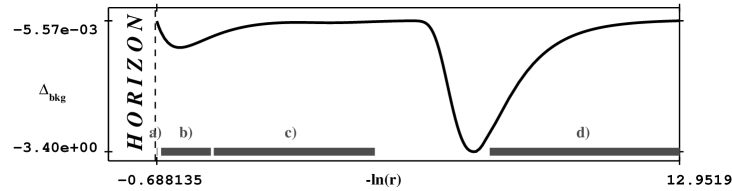
FIG. 1.: Background $\Delta$ under the event horizon. One can see two oscillations of the function $\Delta$ in the “weak oscillation” region (second minimum at $-\ln{r}=3.81671$ is non-observable in this scale) and the first oscillation in the “strong oscillation” region. Although the first fall of $\Delta_{background}$ is not very huge, it is described, however, by the reduced system of equations with a good accuracy and therefore corresponds to the “strong oscillation” regime. Thick grey lines below mark regions depicted in 3-D plots of $\delta\Delta$: a) corresponds to Fig.2, this region is very small; b) corresponds to Fig.3; c) corresponds to Fig.4 and d) corresponds to Fig.5.

We were able to follow the evolution of perturbations of both classes (I and II) with different (small enough) initial amplitudes, propagating through the “weak oscillation” region and the first huge fall of the function $\Delta$ up to a vicinity of the first “almost Cauchy horizon” of the “strong oscillation” region. The common result is that during propagation towards the singularity the considered perturbations do not grow up unboundedly and look like a light ripple on the background solutions. Therefore the strong numerical evidence in favor of nonlinear stability of generic (oscillation type) internal EYM black hole solutions is obtained.

To illustrate this statement we have chosen an appropriate background configuration. Being asymptotically not flat in exterior, it exhibits all important features of EYM black hole interiors and allows one to plot both “weak” and “strong oscillation” regions in the same figure with enough resolution. The chosen background is characterized by the following parameters

$$\begin{array}[]{l}r_{h}=2.0\quad(R=0.5,\quad-\ln{r}=-0.69314718);\\ f_{0}=-0.302072;\\ \sigma_{0}=0.9,\end{array}$$

and the corresponding curve of the metric function $\Delta$ is plotted in Fig. 1.

For the illustration purposes we have used the one-wave class of initial perturbations. According to Section II, it is determined by a $t$ -dependent deviation of the YM function $f$ from its background value which induces the perturbation of $\Pi$; the perturbation of the function $\phi$ is defined to cancel the initial wave, propagating to the negative $t$ -direction.

We plot below the evolution of perturbations with initial parameters in (27):

$$s=100.0;\qquad t_{0}=-10.0$$

for two different amplitudes $K_{1}=10^{-4}$ and $K_{2}=10^{-3}$ in (22) (we will call them “small” and “big” perturbations respectively in the further discussion). These perturbations induce deviations of all other functions according to the full set of EYM equations and the resulting perturbation looks like a nonlinear wave, propagating in the positive spatial $t$ -direction with time $r$, directed to $r\rightarrow 0$.

To show the relative size and shape of perturbations one can normalize the corresponding functions by their equilibrium values. The value $\delta\Delta_{2}$, obtained as $\delta\Delta_{2}=\Delta_{2}-\Delta_{background}$ for “big” initial perturbation, is plotted in four figures: Fig.2, Fig.3, Fig.4 and Fig.5. The considered $r$ - regions are shown in Fig.1 by thick grey lines. The plots illustrate a strongly nonlinear nature of the evolution: the perturbation of the metric function $\Delta$ changes the relative sign and the shape as singularity $r\rightarrow 0$ is approached. The perturbations of other relevant functions behave in a similar way and we do not plot them here.

FIG. 2.: The beginning of the evolution of perturbation of $\delta\Delta_{2}=\Delta_{2}-\Delta_{background}$. The initial perturbation looks like a step. The folds of this step remain to be of a constant height during the beginning of evolution. Further the left fold (greater $t$) will change while the right is constant by definition. This figure corresponds to region a) in Fig.1. The arrow points to the direction of the evolution.

FIG. 3.: Plot of $\delta\Delta_{2}$ in the beginning of the “weak oscillation” region. This figure corresponds to b) region in Fig.1. The arrow points to the direction of the evolution.

FIG. 4.: Plot of $\delta\Delta_{2}$ in the “weak oscillation” region. This figure corresponds to c) region in Fig.1. The arrow points to the direction of the evolution.

FIG. 5.: Plot of $\delta\Delta_{2}$ in the “strong oscillation” region. This figure corresponds to d) region in Fig.1. The arrow points to the direction of the evolution.

However, the perturbations do not grow unboundedly and therefore they do not destroy the background solution. It is convenient to plot the absolute values of the maximal deviation of all relevant functions from their backgrounds as perturbations are developed. The corresponding plots are represented in Figures 6 – 11 for both “small” ($K=10^{-4}$) and “big” ($K=10^{-3}$) initial perturbations along with the background functions.

These plots exhibit most general features of the perturbations, propagating in the different considered generic backgrounds: the evolution of “small” and “big” perturbations looks very similar for all relevant functions, so the difference in initial amplitude does not produce differences in shapes and characters of perturbations; the amplitude of perturbations of $\Delta$ is approximately proportional

FIG. 6.: $\Delta$ background (bottom), absolute value of the maximal deviation from the background (middle – “small” initial perturbation, top – “big” initial perturbation).

FIG. 7.: $\Delta$ in the “weak” oscillation region: background (bottom), absolute value of the maximal deviation from the background (middle – “small” initial perturbation, top – “big” initial perturbation).

FIG. 8.: $\sigma$: background (bottom), absolute value of the maximal deviation from the background (middle – “small” initial perturbation, top – “big” initial perturbation).

FIG. 9.: $f$: background (bottom), absolute value of the maximal deviation from the background (middle – “small” initial perturbation, top – “big” initial perturbation).

to the absolute value of $\Delta$ itself (it grows in the “strong oscillation” regime following the fall of $\Delta_{background}$ and then decreases as $\Delta_{background}$ approaches the “almost Cauchy horizon”); perturbations of all other functions demonstrate bounded nonlinear oscillations in the “weak oscillation” region, then they become almost constant ones in the “strong oscillation” region up to a vicinity of an “almost Cauchy horizon”.

FIG. 10.: $\phi$: background (bottom), absolute value of the maximal deviation from the background (middle – “small” initial perturbation, top – “big” initial perturbation).

FIG. 11.: $\Pi$: absolute value of the maximal deviation from the background (bottom – “small” initial perturbation, top – “big” initial perturbation); the background value of $\Pi$ is zero by definition.

We have followed the evolution of the perturbations towards the $r=0$ singularity up to the first “almost Cauchy horizon” in the “strong oscillation” regime. However, there are no physical reasons to consider the next huge oscillation of the metric function $\Delta$, since in this region the magnitude of the Riemannian squared scalar exceeds the Planckian value ($R_{\mu\nu\lambda\tau}R^{\mu\nu\lambda\tau}>1/L^{4}_{pl.}$) and the classical description of space-time is no longer valid overthere. So, the only problem remains to penetrate numerically through the first “almost Cauchy horizon” in the “strong oscillation” regime. We are going to consider this problem separately along with RN -type using the more precise numerical code.

V Schwarzschild – type solutions

Schwarzschild and Reissner-Nordström types of internal background EYM black hole solutions are of exclusively types since they form a set of zero measure in the space of all initial data [5],[7]. They exist only for some discrete values of ($r_{h}$, $f_{0}$) on a horizon and any internal background solution of (19) with an arbitrary small deviated initial data from these discrete values does correspond to a generic (oscillating) type.

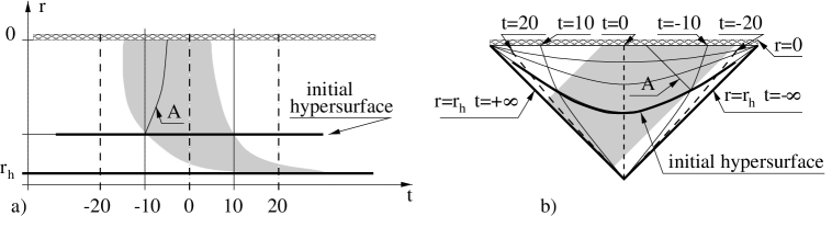
FIG. 12.: The wide table-like perturbation imposed at the initial hypersurface came from the horizon at $t=+\infty$ moves in the negative $t$ -direction (grey region). In the $r,\,t$ coordinates a) the perturbation almost stops its motion in $t$ -direction and only goes with time $r$ to the singularity $r=0$. It will never cross $t=-20$ hypersurface, but it crosses an arbitrary section $t={\rm const}>0$ in the past with necessity, as it follows from the conformal diagram, depicted in b). The top of the “table”, which corresponds to the cross - section $t=0$ can reach the singularity $r=0$ before perturbations from the edges of the initial “table” (curve A) will reach it.

It can be expected that small $t$ -dependent perturbations added to the initial data of these exceptional interiors will produce the transformation to some generic type during the nonlinear evolution towards $r\to 0$. We have investigated the dynamics of perturbations on various Schwarzschild – type EYM black hole internal solutions and convinced ourselves that this transformation really takes place and therefore S-type interiors are occurred to be unstable.

Indeed, according to (24), (26) and (27), the perturbations produce deviations from the background value of the YM function $f$ in the leading order of series expansions with respect to $r$ near the event horizon; it is true by definition for class I and one-wave class of initial perturbations, while the initial perturbations of class II produce similar deviation of the YM function $f$ at the next step on $r$ as perturbation starts to evolve.

Thus, only if waves, produced by the initial perturbation, are suppressed fast enough during their evolution with time $r$ directed towards $r\to 0$, there is a chance for the exceptional internal solution to conserve its S-type. However, our numerical studies show that perturbations are not suppressed during their evolution inward S-type EYM black hole interior and, as a result, S-type singularity transforms to the generic oscillating type.

To illustrate this process it is convenient to investigate S-type interior, perturbed by the initial table-like “outgoing” deviation from the background, which produces the corresponding wave, propagating with time $r$ from $t=+\infty$ to $t<0$. We integrated the equation (17) from the left to the right, the region with large enough negative $t$ corresponds to the originally unperturbed S-type solution since the perturbation never can reach this region [see Fig.12].

Investigating the small $r$ -vicinity of the singularity in different spatial $t$ -regions one can answer the questions about the type of the resulting solution.

We chose the shape of the initial perturbations of $f$ to be a Gauss - like curve, broken at the top by large table - like insertion [see Fig.13]:

FIG. 13.: Initial $f$ perturbation for the Schwarzschild - type solution.

$$\delta f(t)=\left\{\begin{array}[]{ll}Ke^{-s(t-t_{01})^{2}},&t<t_{01},\\ K,&t_{01}\leq t\leq t_{02},\\ Ke^{-s(t-t_{02})^{2}},&t>t_{02}.\\ \end{array}\right.$$

Values of the parameters for the initial data were set equal to:

$$\begin{array}[]{rcl}r_{h}&=&0.613861419,\\ f_{0}&=&-0.8478649145,\\ \sigma_{0}&=&0.289427236,\\ K&=&0.02,\\ t_{01}&=&-10.0,\\ t_{02}&=&10.0.\end{array}$$

This internal background S-type configuration corresponds to the asymptotically flat (black hole) solution with $N=1$ (nodes of YM function) in the external region. We choose the value of $\phi$ in the way that the outgoing wave goes from $t=+\infty$ to $t<0$:

$$\phi(t)=\left\{\begin{array}[]{ll}-d_{1}\sigma_{0}f_{1}h/r_{h}^{2}+2Ks(t-t_{01})e^{-s(t-t_{01})^{2}},&t<t_{01},\\ -d_{1}\sigma_{0}f_{1}h/r_{h}^{2},&t_{01}\leq t\leq t_{02},\\ -d_{1}\sigma_{0}f_{1}h/r_{h}^{2}+2Ks(t-t_{02})e^{-s(t-t_{02})^{2}},&t>t_{02}.\\ \end{array}\right.$$ (29)

This shape of the initial perturbations permits us to investigate three different spatial cross - sections $t=-20$, $t=0$ and $t=20$ independently, since the perturbations from the edges of the initial “table” (at $t=-10$ and $t=10$) can not reach these points during the evolution [see Fig.12].

The solution in the first spatial cross - section corresponds to the background Schwarzschild - type solution. Initial perturbations cannot reach this region, and we obtain the typical Schwarzschild - like behavior [see Fig.14 a) and b)]: the function $\chi$ goes to the constant, approaching the singularity $r=0$ [Fig.14 b)].

The generic - like $\chi$ goes to 0 as $r\to 0$. It is easy to see that the cross - section through the top of the “table” at $t=0$ demonstrates just this type of the behavior [Fig.14 c)], since the considered perturbation are not suppressed during the evolution towards $r\to 0$ and the singularity becomes of the generic (oscillating) type.

FIG. 14.: Various cross - sections of $\chi$ for the Schwarzschild - type internal solution. The cross - section $t=-20$ (a) corresponds to the non-perturbed background solution: approaching the singularity $r=0$, the function $\chi$ goes to the constant (b), while for any generic (oscillating) internal solution the function $\chi$ goes to 0 as $r\to 0$. The cross - sections $t=0$ and $t=+20$ (c), (d) demonstrates that the internal solution becomes the generic one.

Considering a small vicinity of $r=0$, one can see that the resulting solution has already the generic type [Fig.14 d)] also in the third spatial cross - section $t=+20$. The transformation of S-type to the generic one in this region is caused by the shift of the apparent horizon position. The pulse of the considered perturbation shifts the ADM mass of the system and the position of the apparent horizon $r_{h}\rightarrow r_{h}+\delta r_{h}$, while the relevant value of the YM function on the apparent horizon $f_{0}$ remains unperturbed. As a result, new initial data ($r_{h}+\delta r_{h},f_{0}$) for the homogeneous system (19) now corresponds to the generic type of the internal solution.

VI Conclusions

We have investigated the dynamical evolution of small initial perturbations in space-time regions which correspond to internal part of a spherically symmetric black hole in non-Abelian purely magnetic $SU(2)$ EYM theory. The obtained results give a strong numerical evidence in favor of nonlinear stability of the generic (oscillating) type of EYM black hole interiors while the exceptional Schwarzschild - type interiors turn out to be unstable and transform to the generic type as perturbations are developed towards a singularity.

Now one can expect that the generic (oscillating) type of the EYM black hole singularity is stable as well with respect to the perturbations, penetrating into the internal region from the exterior through the event horizon. Moreover, the generic interior solution can pretend to be the final stage of a spherically symmetric collapse of the Yang-Mills field after the event horizon is formed. To check this expectations one should use the null coordinates and the more precise software tools to attack the problem numerically. This work is in progress now.

- [1] R. Penrose, Phys. Rev. Lett. 14, 57 (1965); S. W. Hawking, Proc. R. Soc. London Ser:A300, 187 (1967); S. W. Hawking and R. Penrose, ibid. A314, 529 (1970); S. W. Hawking and G. F. R. Ellis, The Lagre Scale Structure of Space-Time (Cambridge University Press, Cambridge, England, 1973); R. M. Wald, General Relativity (University of Chicago, Chicago, 1984).
- [2] V. A. Belinskii and I. M. Khalatnikov, Zh. Eksp. Teor. Fiz. 56, 1700 (1969) [Sov. Phys. JETP 29, 911 (1969)]; V. A. Belinskii, I. M. Khalatnikov and E. M. Lifshitz, Adv. Phys. 19, 525 (1970); Sov. Phys. Usp. 13, 745 (1971); C. W. Misner, Phys. Rev. Lett. 22, 1071 (1969).
- [3] J. Wainwright and L. Hsu, Class. Quantum Grav. 6, 1409 (1989); C. G. Hewitt and J. Wainwright, Class. Quantum Grav. 10, 99 (1993); A. D. Rendall, Class. Quantum Grav. 14, 2341 (1997).
- [4] M. Weaver, J. Isenberg and B. K. Berger, Phys. Rev. Lett. 80, 2984 (1998); B. Berger, D. Garfinkle, J. Isenberg, V. Moncrief and M. Weaver, Mod. Phys. Lett. A13, 1565 (1998).
- [5] E. E. Donets, D. V. Gal’tsov, and M. Yu. Zotov, Phys. Rev. D56, 3459, (1997).
- [6] D. V. Gal’tsov, E. E. Donets, and M. Yu. Zotov, Pis’ma Zh. Eksp. Teor. Fiz., 65, 855 (1997) [JETP Lett. 65, 895 (1997)].
- [7] P. Breitenlohner, G. Lavrelashvili, and D. Maison, MPI-PhT/97-20, BUTP-97/08, gr-qc/9703047.
- [8] M. S. Volkov and D. V. Gal’tsov, Pis’ma Zh. Eksp. Teor. Fiz. 50, 312 (1989) [JETP Lett. 50, 345 (1990)]; Sov. J. Nucl. Phys. 51, 747 (1990); H. P. Kunzle and A. K. M. Masood-ul-Alam, J. Math. Phys. 31, 928 (1990); P. Bizón, Phys. Rev. Lett. 64, 2844 (1990); P. Breitenlohner, P. Forgács and D. Maison, Commun. Math. Phys. 163, 141 (1994); J. Smoller, A. Wasserman, Commun. Math. Phys. 161, 365 (1994).
- [9] R. Bartnik, J. McKinnon, Phys. Rev. Lett. 61, 141 (1988).
- [10] N. Straumann and Z. Zhou, Phys. Lett. B237, 353, (1990); Phys. Lett. B243, 33 (1990).
- [11] Z. Zhou, N. Straumann, Nucl. Phys. B360, 180 (1991).
- [12] Z. Zhou, Helv. Phys. Acta 65, 767 (1992).
- [13] R. Penrose, in 1968 Battelles Rencontres, edited by B. S. De Witt and J. A. Wheeler (Benjamin, New York, 1968).
- [14] J. M. McNamara, Proc. R. Soc. London A358, 499 (1978); Y. Gürsel, V. D. Sandberg, I. D. Novikov and A. A. Starobinsky, Phys. Rev. D19, 413 (1979); D20, 1260 (1979).
- [15] E. Poisson and W. Israel, Phys. Rev. Lett. 63, 1663 (1989); Phys. Rev. D41, 1796 (1990).
- [16] M. Choptuik, T. Chmaj, P. Bizón, Phys. Rev. Lett. 77, 424 (1996).
- [17] C. Gundlach, Phys. Rev. D55, 6002 (1997).
- [18] L. Burko, Phys. Rev. Lett 79, 4958 (1997); L. Burko and A. Ori, Phys. Rev. D56, 7820 (1997).
- [19] M. Berger and J. Oliger, J. Comput. Phys. 53, 484 (1984).