Abstract

Within a framework of noncommutative geometry, we develop an analogue of (pseudo) Riemannian geometry on finite and discrete sets. On a finite set, there is a counterpart of the continuum metric tensor with a simple geometric interpretation. The latter is based on a correspondence between first order differential calculi and digraphs (the vertices of the latter are given by the elements of the finite set). Arrows originating from a vertex span its (co)tangent space. If the metric is to measure length and angles at some point, it has to be taken as an element of the left-linear tensor product of the space of 1-forms with itself, and not as an element of the (non-local) tensor product over the algebra of functions, as considered previously by several authors. It turns out that linear connections can always be extended to this left tensor product, so that metric compatibility can be defined in the same way as in continuum Riemannian geometry. In particular, in the case of the universal differential calculus on a finite set, the Euclidean geometry of polyhedra is recovered from conditions of metric compatibility and vanishing torsion.

In our rather general framework (which also comprises structures which are far away from continuum differential geometry), there is in general nothing like a Ricci tensor or a curvature scalar. Because of the non-locality of tensor products (over the algebra of functions) of forms, corresponding components (with respect to some module basis) turn out to be rather non-local objects. But one can make use of the parallel transport associated with a connection to ‘localize’ such objects and in certain cases there is a distinguished way to achieve this. In particular, this leads to covariant components of the curvature tensor which allow a contraction to a Ricci tensor. Several examples are worked out to illustrate the procedure. Furthermore, in the case of a differential calculus associated with a hypercubic lattice we propose a new discrete analogue of the (vacuum) Einstein equations.

1 Introduction

In a series of papers [1, 2, 3, 4, 5] we have developed a formalism of differential geometry on finite and discrete sets with applications in particular to lattice gauge theory [6] and discrete completely integrable models [7].

The most basic ‘differential geometric’ structure on a discrete set ${\cal M}$ is a differential calculus $(\Omega({\cal M}),\mbox{d})$, where $\Omega({\cal M})=\bigoplus_{r\geq 0}\Omega^{r}({\cal M})$ is an analogue of the algebra of differential forms on a differentiable manifold and the $\mathbb{C}$-linear map $\mbox{d}\,:\,\Omega^{r}({\cal M})\rightarrow\Omega^{r+1}({\cal M})$ generalizes the exterior derivative. Here ${\cal A}:=\Omega^{0}({\cal M})$ is the algebra of $\mathbb{C}$-valued functions on ${\cal M}$ and noncommutativity enters the stage via nontrivial commutation relations between functions and differentials (which are elements of $\Omega^{1}({\cal M})$). On a discrete set there are many choices of a (first order) differential calculus and it turned out [3] that these amount to the selection of a digraph structure and thus neighbourhood relations on the discrete set.

Whereas the concept of a connection seems to be well understood in the framework of noncommutative geometry, this is not quite so for the concept of a metric. In Connes’ approach to noncommutative geometry [8], Riemannian geometry is encoded in a selfadjoint operator on a Hilbert space and recovered from it via a formula for the distance of two points. The distance formula is then generalized to a more abstract setting, including the case of discrete sets (see also [9] and references therein). A major problem with this approach is that it is bound to (generalizations of) positive definite metrics and thus at least not directly applicable to space-time geometry. The underlying philosophy of ‘spectral geometry’, namely that all geometrical data should be encoded in the spectrum of certain selfadjoint operators on a Hilbert space, is certainly very interesting but by no means compulsive.

In several papers (see [5, 10, 11, 12], for example) a metric in noncommutative geometry has been taken to be an element of the tensor product space $\Omega^{1}({\cal A})\otimes_{\cal A}\Omega^{1}({\cal A})$ with certain properties. Here $\Omega^{1}({\cal A})$ is the space of 1-forms of a differential calculus over an associative algebra ${\cal A}$. This has just been a formal generalization of one of several, in classical differential geometry equivalent, definitions of a metric tensor field, motivated by simplicity of mathematical structure but without a deeper, e.g. physical, substantiation. Even on the technical level a serious problem showed up, namely the extensibility of a (linear) connection on $\Omega^{1}({\cal A})$ to a connection on $\Omega^{1}({\cal A})\otimes_{\cal A}\Omega^{1}({\cal A})$, which is necessary in order to define metric compatibility of a linear connection (see [5, 13] for discussions and related references).

Needless to say, generalizing another – classically equivalent – metric concept, one does not in general arrive at equivalent structures in the noncommutative geometric setting. In fact, motivated by previous work [6, 7] we recently investigated in more detail generalizations of the Hodge $\star$-operator [14]. The metric is recovered from $(\alpha,\beta)=\star^{-1}(\alpha\star\beta)$ where $\alpha,\beta$ are differential 1-forms. For a symmetric Hodge operator on a (noncommutative) differential calculus over a commutative algebra ${\cal A}$, contact was made with a metric defined as an element

$$g\in\Omega^{1}({\cal A})\otimes_{L}\Omega^{1}({\cal A})$$ (1.1)

and not as an element of the space $\Omega^{1}({\cal A})\otimes_{\cal A}\Omega^{1}({\cal A})$. The tensor product $\otimes_{L}$ satisfies

$$(f\,\alpha)\otimes_{L}(h\,\beta)=f\,h\,(\alpha\otimes_{L}\beta)\qquad\forall f,h\in{\cal A},\,\alpha,\beta\in\Omega({\cal A})\;.$$ (1.2)

In the following we show that it is precisely the latter metric definition which directly reproduces some familiar results in discrete geometry and which allows us to develop discrete noncommutative geometry to a more satisfactory level. It should be noticed, however, that the tensor product $\otimes_{L}$ and therefore the metric definition (1.1) does not generalize in an obvious way to noncommutative algebras ${\cal A}$, at least as far as we can see. But in [14] we have generalized the associated Hodge operator to the general noncommutative framework.

In section 2 we recall some basic definitions of noncommutative geometry. Section 3 concentrates on finite sets and introduces metrics and compatible linear connections on them. Section 4 deals with a technical problem which has its origin in the non-locality of the tensor product over ${\cal A}$. In particular, the construction of a Ricci tensor is addressed in our framework. As an example of particular interest, the geometry of a hypercubic lattice is treated in section 5. Section 6 deals with discrete surfaces of revolution. Some conclusions are collected in section 7. In particular, we propose a new discrete version of the Einstein equations on a hypercubic lattice.

2 Preliminaries

In the first subsection we recall the definition of a differential calculus over an associative algebra. The second subsection contains the general definitions of linear connections, torsion and curvature in the framework of noncommutative geometry.

2.1 Differential calculi on associative algebras

Let ${\cal A}$ be an associative algebra over $\mathbb{C}$ with unit ${\leavevmode{\rm 1\mkern-5.4muI}}$. A differential calculus over ${\cal A}$ is a $\mathbb{Z}$-graded associative algebra (over $\mathbb{C}$)

$$\Omega({\cal A})=\bigoplus_{r\geq 0}\Omega^{r}({\cal A})$$ (2.1)

where the spaces $\Omega^{r}({\cal A})$ are ${\cal A}$-bimodules and $\Omega^{0}({\cal A})={\cal A}$. There is a $\mathbb{C}$-linear map

$$\mbox{d}\;:\quad\Omega^{r}({\cal A})\rightarrow\Omega^{r+1}({\cal A})$$ (2.2)

with the following properties,

$$\mbox{d}^{2} = 0$$ (2.3)

$$\mbox{d}(w\,w^{\prime}) = (\mbox{d}w)\,w^{\prime}+(-1)^{r}\,w\,\mbox{d}w^{\prime}$$ (2.4)

where $w\in\Omega^{r}({\cal A})$ and $w^{\prime}\in\Omega({\cal A})$. The last relation is known as the (generalized) Leibniz rule. One also requires ${\leavevmode{\rm 1\mkern-5.4muI}}\,w=w\,{\leavevmode{\rm 1\mkern-5.4muI}}=w$ for all elements $w\in\Omega({\cal A})$. The identity ${\leavevmode{\rm 1\mkern-5.4muI}}{\leavevmode{\rm 1\mkern-5.4muI}}={\leavevmode{\rm 1\mkern-5.4muI}}$ then implies

$$\mbox{d}{\leavevmode{\rm 1\mkern-5.4muI}}=0\;.$$ (2.5)

Furthermore, we require that d generates the spaces $\Omega^{r}({\cal A})$ for $r>0$ in the sense that $\Omega^{r}({\cal A})={\cal A}\,\mbox{d}\Omega^{r-1}({\cal A})\,{\cal A}$.

2.2 Linear connections, torsion, and curvature

Let $(\Omega({\cal A}),\mbox{d})$ be a differential calculus over an associative algebra ${\cal A}$. A linear (left ${\cal A}$-module) connection is a $\mathbb{C}$-linear map $\nabla\,:\,\Omega^{1}({\cal A})\rightarrow\Omega^{1}({\cal A})\otimes_{\cal A}\Omega({\cal A})$ such that

$$\nabla(f\,\alpha)=\mbox{d}f\otimes_{\cal A}\alpha+f\,\nabla\alpha\;.$$ (2.6)

A linear connection extends to a map $\nabla\,:\,\Omega({\cal A})\otimes_{\cal A}\Omega^{1}({\cal A})\rightarrow\Omega({\cal A})\otimes_{\cal A}\Omega^{1}({\cal A})$ via

$$\nabla(w\otimes_{\cal A}\alpha)=\mbox{d}w\otimes_{\cal A}\alpha+(-1)^{r}\,w\,\nabla\alpha\qquad\quad\forall w\in\Omega^{r}({\cal A}),\,\alpha\in\Omega^{1}({\cal A})\;.$$ (2.7)

The torsion of a linear connection $\nabla$ is the map $\Theta\,:\,\Omega^{1}({\cal A})\rightarrow\Omega^{2}({\cal A})$ given by

$$\Theta(\alpha):=\mbox{d}\alpha-\pi\circ\nabla\alpha$$ (2.8)

where $\pi$ is the natural projection $\Omega^{1}({\cal A})\otimes_{\cal A}\Omega^{1}({\cal A})\rightarrow\Omega^{2}({\cal A})$. It satisfies

$$\Theta(f\,\alpha)=f\,\Theta(\alpha)\;.$$ (2.9)

The torsion extends to a map $\Theta\,:\,\Omega({\cal A})\otimes_{\cal A}\Omega^{1}({\cal A})\rightarrow\Omega({\cal A})$ via

$$\Theta(w\otimes_{\cal A}\alpha):=\mbox{d}(w\,\alpha)-\pi\circ\nabla(w\otimes_{\cal A}\alpha)\qquad\forall w\in\Omega({\cal A}),\,\alpha\in\Omega^{1}({\cal A})$$ (2.10)

where $\pi$ now denotes more generally the projection $\Omega({\cal A})\otimes_{\cal A}\Omega^{1}({\cal A})\rightarrow\Omega({\cal A})$. Then

$$\Theta(\nabla\alpha) = \mbox{d}\pi\circ\nabla(\alpha)-\pi\circ\nabla^{2}(\alpha)$$ (2.11)

$$= \mbox{d}(\mbox{d}\alpha-\Theta(\alpha))+\pi\circ\mathfrak{R}(\alpha)$$

where we have introduced the curvature $\mathfrak{R}$ of $\nabla$ as the map

$$\mathfrak{R}:=-\nabla^{2}$$ (2.12)

which satisfies

$$\mathfrak{R}(f\,\alpha)=f\,\mathfrak{R}(\alpha)\;.$$ (2.13)

We arrive at the first Bianchi identity

$$\mbox{d}\circ\Theta+\Theta\circ\nabla=\pi\circ\mathfrak{R}\;.$$ (2.14)

The second Bianchi identity is

$$(\nabla\mathfrak{R})(\alpha):=\nabla(\mathfrak{R}(\alpha))-\mathfrak{R}(\nabla\alpha)=-\nabla^{3}\alpha+\nabla^{3}\alpha=0\;.$$ (2.15)

Example. For the universal differential calculus, we have $\pi=\mbox{id}$ on $\Omega^{1}\otimes_{\cal A}\Omega^{1}$ and there is a unique linear connection with vanishing torsion given by $\nabla=\mbox{d}$ according to (2.8). The curvature of this linear connection vanishes. $\blacksquare$

3 Differential geometry on finite sets

In this section we collect some facts about differential calculi, vector fields and linear connections on finite sets (see also [2, 3, 4, 5, 15, 16]). We then consider metrics and elaborate the metric compatibility condition for a linear connection.

3.1 First order differential calculi on a finite set

Let ${\cal M}$ be a finite set of $N$ elements and ${\cal A}$ the algebra of all $\mathbb{C}$-valued functions on it. ${\cal A}$ is a complex linear space with basis $e^{i},\,i=1,\ldots,N$, where $e^{i}(j)=\delta^{i}_{j}$ for $i,j\in\cal M$. These functions satisfy the two identities

$$e^{i}\,e^{j}=\delta^{ij}\,e^{j}\,,\qquad\sum_{i}e^{i}={\leavevmode{\rm 1\mkern-5.4muI}}$$ (3.1)

where ${\leavevmode{\rm 1\mkern-5.4muI}}$ is the constant function on ${\cal M}$ with value 1. In [3] it has been shown that first order differential calculi on a finite set ${\cal M}$ are in bijective correspondence with digraph structures on ${\cal M}$. Given a digraph with set of vertices ${\cal M}$, we associate with an arrow from some point $i$ to another point $j$, denoted as $i\longrightarrow j$ in the following, an algebraic object $e^{ij}$ and define

$$\Omega^{1}:=\mbox{span}_{\mathbb{C}}\{e^{ij}\,\mid\,i\longrightarrow j\}\;.$$ (3.2)

This is turned into an ${\cal A}$-bimodule via

$$e^{i}\,e^{kl}=\delta^{ik}\,e^{kl}\,,\quad e^{kl}\,e^{i}=\delta^{li}\,e^{kl}\;.$$ (3.3)

Let us introduce

$$\rho=\sum_{k,l}e^{kl}$$ (3.4)

where the summation has to be restricted to those $k,l$ for which there is an arrow from $k$ to $l$ in the digraph. Then

$$\mbox{d}f=[\rho,f]\qquad\qquad f\in{\cal A}$$ (3.5)

defines a $\mathbb{C}$-linear map $\mbox{d}\,:\,{\cal A}\rightarrow\Omega^{1}$ which satisfies the Leibniz rule. If there is an arrow from $i$ to $j$ in the digraph, then $e^{i}\rho\,e^{j}=e^{ij}$, otherwise $e^{i}\rho\,e^{j}=0$.

The subspace

$$\Omega^{1}_{i}:=e^{i}\,\Omega^{1}$$ (3.6)

is generated by the 1-forms $e^{ij}$ corresponding to the arrows originating from $i$ in the digraph. It may be regarded as the cotangent space at $i\in{\cal M}$. We have

$$\Omega^{1}=\bigoplus_{i\in{\cal M}}\Omega^{1}_{i}\;.$$ (3.7)

The complete digraph where all pairs of points in ${\cal M}$ are connected by a pair of antiparallel arrows corresponds to the largest first order differential calculus on ${\cal M}$, also known as the universal first order differential calculus since each other calculus can be obtained from it as a quotient with respect to some sub-bimodule.

There is a canonical commutative product in $\Omega^{1}$ which satisfies

$$\alpha\bullet\mbox{d}f=[\alpha,f]$$ (3.8)

and

$$(f\,\alpha\,f^{\prime})\bullet(h\,\beta\,h^{\prime})=fh\,(\alpha\bullet\beta)\,f^{\prime}h^{\prime}\qquad\qquad\forall f,f^{\prime},h,h^{\prime}\in{\cal A},\,\alpha,\beta\in\Omega^{1}\;.$$ (3.9)

More generally, this product exists for every first order differential calculus over a commutative algebra [17]. In the case under consideration, it is given by

$$e^{ij}\bullet e^{kl}=\delta^{ik}\,\delta^{jl}\,e^{ij}\;.$$ (3.10)

The space of 1-forms $\Omega^{1}$ is free as a (left or right) ${\cal A}$-modul. A special left ${\cal A}$-module basis is given by

$$\rho^{i}:=\sum_{j}\,e^{ji}\qquad\mbox{if }\rho\,e^{i}\neq 0$$ (3.11)

since an arbitrary 1-form $A$ can be written as

$$A=\sum_{ij}A_{ij}e^{ij}=\sum_{i}A_{i}\,\rho^{i}$$ (3.12)

where $A_{i}=\sum_{j}A_{ji}\,e^{j}$. Furthermore, $\sum_{i}A_{i}\,\rho^{i}=0$ implies, via multiplication with $e^{j}$ from the left, that $A_{ji}=0$ and thus $A_{i}=0$.

3.2 Higher order differential forms on a finite set

Concatenation of the 1-forms $e^{ij}$ leads to the $r$-forms

$$e^{i_{0}\ldots i_{r}}:=e^{i_{0}i_{1}}\,e^{i_{2}i_{3}}\cdots e^{i_{r-1}i_{r}}\qquad(r>0)$$ (3.13)

which can also be expressed as follows,

$$e^{i_{0}\ldots i_{r}}=e^{i_{0}}\,\rho\,e^{i_{1}}\,\rho\,\cdots\,\rho\,e^{i_{r}}\;.$$ (3.14)

They satisfy the simple relations

$$e^{i_{0}\ldots i_{r}}\,e^{j_{0}\ldots j_{s}}=\delta^{i_{r}j_{0}}\,e^{i_{0}\ldots i_{r-1}j_{0}\ldots j_{s}}$$ (3.15)

and span $\Omega^{r}$ as a vector space over $\mathbb{C}$. Using (3.3) this space is turned into an ${\cal A}$-bimodule. The exterior derivative d extends to higher orders via

$$\mbox{d}e^{i} = \rho\,e^{i}-e^{i}\,\rho$$ (3.16)

$$\mbox{d}\rho = \rho^{2}+\sum_{i}e^{i}\,\rho^{2}\,e^{i}$$ (3.17)

and the (graded) Leibniz rule (2.4). In particular, this leads to

$$\mbox{d}e^{ij} = \rho\,e^{i}\,\rho\,e^{j}-e^{i}\,\rho^{2}e^{j}+e^{i}\,\rho\,e^{j}\,\rho$$ (3.18)

$$\mbox{d}e^{ijk} = \rho\,e^{i}\,\rho\,e^{j}\,\rho\,e^{k}-e^{i}\,\rho^{2}e^{j}\,\rho\,e^{k}+e^{i}\,\rho\,e^{j}\,\rho^{2}e^{k}-e^{i}\,\rho\,e^{j}\,\rho\,e^{k}\,\rho\;.$$ (3.19)

Starting with the universal first order differential calculus on ${\cal M}$, these formulas generate the universal differential calculus (which is also known as the universal differential envelope of ${\cal A}$). A smaller first order differential calculus (where some of the $e^{ij}$ are missing) induces restrictions on the spaces of higher order forms. A missing arrow from $i$ to some other point $j$ (in the complete digraph on ${\cal M}$) means $e^{i}\rho\,e^{j}=0$. Acting with d on this equation, using (3.16) and (3.17), leads to

$$i\,\not\!\!\longrightarrow\,j\quad\Rightarrow\quad e^{i}\,\rho^{2}\,e^{j}=0\;.$$ (3.20)

Each differential calculus is obtained from the universal one as a quotient with respect to some differential ideal. If the differential ideal is generated by ‘basic forms’ (3.13) only, then the differential calculus is called basic [16]. This class of differential calculi has been associated with polyhedral representations of simplicial complexes [16].

3.3 Vector fields on a finite set

Let $\mathfrak{X}$ denote the dual of $\Omega^{1}$ as a complex vector space. Let $\{\partial_{ji}\}$ be the basis of $\mathfrak{X}$ dual to $\{e^{ij}\}$. If $\langle\,,\rangle_{0}$ denotes the duality contraction, then

$$\langle e^{ij},\partial_{kl}\rangle_{0}=\delta^{i}_{l}\,\delta^{j}_{k}\;.$$ (3.21)

$\mathfrak{X}$ is turned into an ${\cal A}$-bimodule by introducing the left and right actions

$$\langle\alpha,f\cdot X\rangle_{0}:=\langle\alpha f,X\rangle_{0}\;,\qquad\langle\alpha,X\cdot f\rangle_{0}:=\langle f\alpha,X\rangle_{0}\;.$$ (3.22)

As a consequence,

$$e^{k}\cdot\partial_{ji}=\delta^{k}_{j}\,\partial_{ji}\,,\qquad\partial_{ji}\cdot e^{k}=\delta^{k}_{i}\,\partial_{ji}\;.$$ (3.23)

An element $X\in\mathfrak{X}$ can be uniquely decomposed as follows,

$$X=\sum_{i\longrightarrow j}X(i)^{j}\,\partial_{ji}$$ (3.24)

(where the summation runs over all $i,j\in{\cal M}$ for which there is an arrow from $i$ to $j$ in the digraph associated with $\Omega^{1}$). Now we introduce a duality contraction $\langle\,,\rangle$ of $\Omega^{1}$ as a right ${\cal A}$-module and $\mathfrak{X}$ as a left ${\cal A}$-module by setting

$$\langle e^{ij},X\rangle:=e^{i}\,\langle e^{ij},X\rangle_{0}$$ (3.25)

for all $X\in\mathfrak{X}$. Then we have

$$\langle f\alpha,X\cdot h\rangle=f\,\langle\alpha,X\rangle\,h\,,\qquad\langle\alpha,f\cdot X\rangle=\langle\alpha f,X\rangle\;.$$ (3.26)

The elements of $\mathfrak{X}$ become operators on ${\cal A}$ via

$$X(f):=\langle\mbox{d}f,X\rangle\;.$$ (3.27)

Using the Leibniz rule for d, one proves

$$X(fh)=f\,X(h)+(h\cdot X)(f)\qquad\qquad\forall f,h\in{\cal A}\;.$$ (3.28)

Furthermore,

$$(X\cdot f)(g)=X(g)\,f\;.$$ (3.29)

The duality contraction extends to the pair of spaces $\Omega\otimes_{\cal A}\Omega^{1}$ and $\mathfrak{X}\otimes_{\cal A}\Omega$ via

$$\langle w\otimes_{\cal A}\alpha,X\otimes_{\cal A}w^{\prime}\rangle=w\,\langle\alpha,X\rangle\,w^{\prime}\;.$$ (3.30)

The space

$$\mathfrak{X}_{i}:=\mathfrak{X}\,e^{i}=\{X\cdot e^{i}\,|\,X\in\mathfrak{X}\}$$ (3.31)

may be regarded as the tangent space at $i\in{\cal M}$. It is dual to $\Omega_{i}^{1}$ with respect to the duality contraction $\langle\;,\,\rangle_{0}$. The set $\{\partial_{ji}\,|\,j\in{\cal M}\;\mbox{such that}\;i\longrightarrow j\}$ is a basis of $\mathfrak{X}_{i}$ which is dual to the basis $\{e^{ij}\,|\,j\in{\cal M}\;\mbox{such that}\;i\longrightarrow j\}$ of $\Omega_{i}^{1}$.

3.4 Linear connections on a finite set

Let $\nabla\,:\,\Omega^{1}\rightarrow\Omega^{1}\otimes_{\cal A}\Omega^{1}$ be a (left ${\cal A}$-module) linear connection. Using (2.6) and the properties of $\rho$, one finds that

$$\mathbb{U}(\alpha):=\rho\otimes_{\cal A}\alpha-\nabla\alpha$$ (3.32)

is a left ${\cal A}$-homomorphism $\mathbb{U}\,:\,\Omega^{1}\rightarrow\Omega^{1}\otimes_{\cal A}\Omega^{1}$, i.e.,

$$\mathbb{U}(f\alpha)=f\,\mathbb{U}(\alpha)\qquad\forall f\in{\cal A},\,\alpha\in\Omega^{1}\;.$$ (3.33)

We call $\mathbb{U}$ the parallel transport associated with the linear connection $\nabla$. In particular, (3.33) implies $\mathbb{U}(e^{ij})=e^{i}\,\mathbb{U}(e^{ij})$ and thus we have an expansion

$$\mathbb{U}(e^{ij})=\sum_{k,l}U(i)^{j}{}_{kl}\,e^{ik}\otimes_{\cal A}e^{kl}=\sum_{k}e^{ik}\otimes_{\cal A}\sum_{l}U(i)^{j}{}_{kl}\,e^{kl}$$ (3.34)

with constants $U(i)^{j}{}_{kl}$.

Via

$$e^{ik}\quad\mapsto\quad(e^{ik})\mathbb{U}^{ij}:=\sum_{l}U(i)^{k}{}_{jl}\,e^{jl}$$ (3.35)

for fixed $i$ and $j$, the parallel transport defines a linear map $\Omega^{1}_{i}\rightarrow\Omega^{1}_{j}$ with associated matrix $\mathbb{U}^{ij}$. Then we have

$$\mathbb{U}(\alpha)=\sum_{i,j}e^{ij}\otimes_{\cal A}[(e^{i}\,\alpha)\mathbb{U}^{ij}]\;.$$ (3.36)

Given a linear connection on $\Omega^{1}$, there is a dual connection $\nabla\,:\,\mathfrak{X}\rightarrow\mathfrak{X}\otimes_{\cal A}\Omega^{1}$, such that

$$\mbox{d}\langle\alpha,X\rangle=\langle\nabla\alpha,X\rangle+\langle\alpha,\nabla X\rangle$$ (3.37)

(cf [5], appendix B). Using $\mbox{d}\langle\alpha,X\rangle=[\rho,\langle\alpha,X\rangle]$ one proves that the dual parallel transport defined by

$$\langle\alpha,\mathbb{U}(X)\rangle=\langle\mathbb{U}(\alpha),X\rangle$$ (3.38)

acts as follows on $\mathfrak{X}$,

$$\mathbb{U}(X):=X\otimes_{\cal A}\rho+\nabla X\,,$$ (3.39)

and satisfies

$$\mathbb{U}(X\cdot f)=\mathbb{U}(X)\,f\;.$$ (3.40)

(3.34) leads to

$$\mathbb{U}(\partial_{ji})=\sum_{k,l}U(k)^{l}{}_{ij}\,\partial_{lk}\otimes_{\cal A}e^{ki}\;.$$ (3.41)

The parallel transport (and thus also the connection) extends in an obvious way to $\Omega\otimes_{\cal A}\Omega^{1}$ and $\mathfrak{X}\otimes_{\cal A}\Omega$ as graded left respectively right $\Omega$-homomorphisms, i.e.,

$$\mathbb{U}(w\otimes_{\cal A}\alpha)=(-1)^{r}\,w\otimes_{\cal A}\mathbb{U}(\alpha)\;,\qquad\mathbb{U}(X\otimes_{\cal A}w)=(-1)^{r}\,\mathbb{U}(X)\otimes_{\cal A}w$$ (3.42)

where $w\in\Omega^{r}$.

The map $\mathfrak{X}_{j}\rightarrow\mathfrak{X}_{i}$ dual to the parallel transport map with matrix $\mathbb{U}^{ij}$ defined in (3.35) is given by

$$\partial_{ki}\quad\mapsto\quad\sum_{l}U(j)^{l}_{ik}\,\partial_{lj}=\mathbb{U}^{ij}(\partial_{ki})\;.$$ (3.43)

Now (3.41) extends to

$$\mathbb{U}(X)=\sum_{i,j}\mathbb{U}^{ij}(X\cdot e^{i})\otimes_{\cal A}e^{ij}\;.$$ (3.44)

We may introduce the curvature as the right $\Omega$-homomorphism $\mathfrak{R}^{\prime}\,:\,\mathfrak{X}\otimes_{\cal A}\Omega\rightarrow\mathfrak{X}\otimes_{\cal A}\Omega$ defined by

$$\mathfrak{R}^{\prime}=\nabla^{2}\;.$$ (3.45)

Its dual $\mathfrak{R}:\Omega\otimes_{\cal A}\Omega^{1}\rightarrow\Omega\otimes_{\cal A}\Omega^{1}$ is then given by $\mathfrak{R}=-\nabla^{2}$ in accordance with our general definition (2.12). We obtain

$$\mathfrak{R}(e^{ij}) =: \sum_{k,l,m}R(i)^{j}{}_{klm}\,e^{ikl}\otimes_{\cal A}e^{lm}$$ (3.46)

$$= \sum_{k,l,m}\left(\sum_{n}U(i)^{j}{}_{kn}\,U(k)^{n}{}_{lm}-U(i)^{j}{}_{lm}\right)\,e^{ikl}\otimes_{\cal A}e^{lm}$$

where it has been convenient to set

$$U(i)^{j}{}_{ik}:=\delta^{j}_{k}\;.$$ (3.47)

We also have the following expression for the curvature,

$$\mathfrak{R}(\alpha)=\sum_{i,j,k}e^{ijk}\otimes_{\cal A}\bigl{\{}(e^{i}\,\alpha)[\mathbb{U}^{ij}\,\mathbb{U}^{jk}-\mathbb{U}^{ik}]\bigr{\}}$$ (3.48)

where $\mathbb{U}^{ii}:={\rm id}_{\Omega^{1}_{i}}$.

For the torsion we find

$$\Theta(e^{ij})=-e^{i}\rho^{2}e^{j}+e^{ij}\,\rho+\sum_{k,l}U(i)^{j}{}_{kl}\,e^{ikl}=\sum_{k,l}(\delta^{j}_{k}-\delta^{j}_{l}+U(i)^{j}{}_{kl})\,e^{ikl}\;.$$ (3.49)

Example. In case of the universal differential calculus, the condition of vanishing torsion leads to

$$U(i)^{j}{}_{kl}=\delta^{j}_{l}-\delta^{j}_{k}$$ (3.50)

and thus fixes the linear connection completely. As mentioned in more generality in the example in section 2.2, this connection is given by $\nabla=\mbox{d}$ and its curvature vanishes. $\blacksquare$

3.5 Metrics and compatible linear connections on finite sets

Using

$$e^{ij}\otimes_{L}e^{kl}=e^{ij}\otimes_{L}e^{k}\,e^{kl}=e^{k}\,e^{ij}\otimes_{L}e^{kl}=\delta^{ki}\,e^{ij}\otimes_{L}e^{il}$$ (3.51)

one finds that an element $g\in\Omega^{1}\otimes_{L}\Omega^{1}$ can be expressed as

$$g=\sum_{i,j,k}g(i)_{jk}\,e^{ij}\otimes_{L}e^{ik}$$ (3.52)

with constants $g(i)_{jk}$. This will be our candidate for a metric on ${\cal M}$.

Example 1. Consider a digraph embedded in Euclidean space such that the arrows are straight lines of Euclidean length $\ell_{ij}$. Let $\vartheta_{jik}$ denote the angle between arrows from $i$ to $j$ and from $i$ to $k$. Define

$$g(i)_{jj}=\ell_{ij}^{2}\,,\qquad g(i)_{jk}=\ell_{ij}\,\ell_{ik}\,\cos\vartheta_{jik}\;.$$ (3.53)

In order to describe the geometry of a polygon (without orientation of its lines) embedded in Euclidean space completely, in general we need to associate it with a symmetric digraph. A line between two points $i$ and $j$ is then represented by a pair of antiparallel arrows, so that $e^{ij}$ and $e^{ji}$ are both present. Of course, we should impose $\ell_{ij}=\ell_{ji}$. $\blacksquare$

In order to define compatibility of a linear connection and a metric, we have to extend the connection, respectively the map $\mathbb{U}$, from $\Omega^{1}$ to $\Omega^{1}\otimes_{L}\Omega^{1}$. Let us define

$$\mathbb{U}(\alpha\otimes_{L}\beta):=\bullet\left(\mathbb{U}(\alpha)\otimes_{L}\mathbb{U}(\beta)\right)$$ (3.54)

where a map

$$\bullet\,:\,(\Omega^{1}\otimes_{\cal A}\Omega^{1})\otimes_{L}(\Omega^{1}\otimes_{\cal A}\Omega^{1})\rightarrow\Omega^{1}\otimes_{\cal A}(\Omega^{1}\otimes_{L}\Omega^{1})$$ (3.55)

is needed. Using the canonical product (3.10) in the space of 1-forms, such a map is given by

$$\bullet\left((\alpha\otimes_{\cal A}\beta)\otimes_{L}(\alpha^{\prime}\otimes_{\cal A}\beta^{\prime})\right):=(\alpha\bullet\alpha^{\prime})\otimes_{\cal A}(\beta\otimes_{L}\beta^{\prime})$$ (3.56)

and, using (3.9), we have

$$\mathbb{U}(f\,(\alpha\otimes_{L}\beta))=f\,\mathbb{U}(\alpha\otimes_{L}\beta)\;.$$ (3.57)

As a consequence,

$$\nabla(\alpha\otimes_{L}\beta):=\rho\otimes_{\cal A}(\alpha\otimes_{L}\beta)-\mathbb{U}(\alpha\otimes_{L}\beta)$$ (3.58)

defines a (left ${\cal A}$-module) connection on $\Omega^{1}\otimes_{L}\Omega^{1}$. The metric compatibility condition $\nabla g=0$ now amounts to

$$\rho\otimes_{\cal A}g=\mathbb{U}(g)\;.$$ (3.59)

In terms of the matrices $\mathbb{U}^{ij}$ introduced in section 3.4, we have

$$\mathbb{U}(\alpha\otimes_{L}\beta)=\sum_{i,j}e^{ij}\otimes_{\cal A}\bigl{\{}[(e^{i}\alpha)\mathbb{U}^{ij}]\otimes_{L}(e^{i}\,\beta)\mathbb{U}^{ij}]\bigr{\}}\;.$$ (3.60)

Lemma. Expressed in components, $\nabla g=0$ becomes

$$g(i)_{jk}=\sum_{m,n}g(l)_{mn}\,U(l)^{m}{}_{ij}\,U(l)^{n}{}_{ik}$$ (3.61)

for all $i,l\in{\cal M}$ such that $l\longrightarrow i$ (i.e., there is an arrow from $l$ to $i$ in the digraph associated with $\Omega^{1}$). Proof.

$$\mathbb{U}(g) = \sum_{l,m,n}g(l)_{mn}\,\bullet(\mathbb{U}(e^{lm})\otimes_{L}\mathbb{U}(e^{ln}))$$

$$= \sum_{l,m,n}g(l)_{mn}\,\sum_{i,j,k,p}U(l)^{m}{}_{ij}\,U(l)^{n}{}_{pk}\,\bullet((e^{li}\otimes_{\cal A}e^{ij})\otimes_{L}(e^{lp}\otimes_{\cal A}e^{pk}))\;.$$

With

$$\bullet((e^{li}\otimes_{\cal A}e^{ij})\otimes_{L}(e^{lp}\otimes_{\cal A}e^{pk})) = (e^{li}\bullet e^{lp})\otimes_{\cal A}(e^{ij}\otimes_{L}e^{pk})$$

$$= \delta^{ip}\,e^{li}\otimes_{\cal A}(e^{ij}\otimes_{L}e^{pk})$$

this becomes

$$\mathbb{U}(g)=\sum_{i,j,k,l,m,n}g(l)_{mn}\,U(l)^{m}{}_{ij}\,U(l)^{n}{}_{ik}\,e^{li}\otimes_{\cal A}(e^{ij}\otimes_{L}e^{ik})\;.$$

Using (3.59), the last expression must be equal to

$$\rho\otimes_{\cal A}g=\sum_{i,j,k,l}g(i)_{jk}\,e^{li}\otimes_{\cal A}(e^{ij}\otimes_{L}e^{ik})\;.$$

Comparison of the coefficients on both sides now leads to our formula. $\blacksquare$

Example 2. Again, we consider the universal differential calculus on ${\cal M}$. With the unique torsion-free linear connection (3.50), the metric compatibility condition reads

$$g(i)_{kl}=g(j)_{kl}+g(j)_{ii}-g(j)_{ki}-g(j)_{il}\qquad i,j,k,l\in{\cal M}\;.$$ (3.62)

Setting $k=j$ and $l=j$, respectively, we get

$$g(i)_{jk}=g(j)_{ii}-g(j)_{ik}\,,\qquad g(i)_{kj}=g(j)_{ii}-g(j)_{ki}$$ (3.63)

which in turn implies

$$g(i)_{jk}-g(i)_{kj}=g(j)_{ki}-g(j)_{ik}$$ (3.64)

and

$$g(i)_{jj}=g(j)_{ii}\;.$$ (3.65)

Furthermore, the last equation together with (3.62) leads to

$$2\,g(i)_{kl}-g(i)_{kj}-g(i)_{jl}=2\,g(j)_{kl}-g(j)_{ki}-g(j)_{il}$$ (3.66)

which for $k=l$ becomes

$$2\,g(i)_{kk}-g(i)_{kj}-g(i)_{jk}=2\,g(j)_{kk}-g(j)_{ki}-g(j)_{ik}\;.$$ (3.67)

Let us now consider the special case where all the components $g(i)_{jj}$ are equal. Then (3.64) and (3.67) lead to

$$g(i)_{kj}=g(j)_{ik}\;.$$ (3.68)

With the help of (3.63) and (3.65) we now obtain

$$g(i)_{jj}=g(i)_{jk}+g(i)_{kj}\;.$$ (3.69)

Assuming in addition that the metric is symmetric (i.e., $g(i)_{jk}=g(i)_{kj}$), we have

$$g(i)_{jj}=2\,g(i)_{jk}$$ (3.70)

and we end up with a constant metric

$$g(i)=\left(\begin{array}[]{cccc}a&a/2&\ldots&a/2\\ a/2&\ddots&&\vdots\\ \vdots&&\ddots&\vdots\\ a/2&\cdots&a/2&a\end{array}\right)\qquad\qquad\forall i\in{\cal M}\;.$$ (3.75)

Hence, there is a unique symmetric $g$ for the universal differential calculus (associated with the complete digraph) on ${\cal M}$ which is compatible with the (unique) torsion-free linear connection and which has the property that all $g(i)_{jj}$ are equal. If $g(i)_{jj}$ is positive, we let it represent the square of the distance between $i$ and $j$. The above requirement then means that all points are at equal distance $\ell=\sqrt{a}$ and from the metric compatibility condition we recover the Euclidean geometry of the regular polyhedron.

More generally, specializing to the ‘Euclidean metric’ (3.53), our metric compatibility conditions (3.62) become

$$\ell_{ik}^{2} = \ell_{jk}^{2}+\ell_{ji}^{2}-2\,\ell_{ji}\ell_{jk}\,\cos(\vartheta_{ijk})$$ (3.76)

$$\ell_{ik}\ell_{il}\,\cos(\vartheta_{kil}) = \ell_{jk}\ell_{jl}\,\cos(\vartheta_{kjl})+\ell_{ji}^{2}-\ell_{ji}\ell_{jk}\,\cos(\vartheta_{ijk})-\ell_{ji}\ell_{jl}\,\cos(\vartheta_{ijl})\quad$$ (3.77)

which in fact reproduce well-known relations of Euclidean geometry. $\blacksquare$

In terms of the matrices

$$g(i):=(g(i)_{jk})$$ (3.78)

the metric compatibility condition takes the simple form

$$g(j)=(\mathbb{U}^{ij})^{t}\,g(i)\,\mathbb{U}^{ij}$$ (3.79)

where $(\mathbb{U}^{ij})^{t}$ denotes the transpose of the matrix $\mathbb{U}^{ij}$. Hence, if there is an arrow from $i$ to $j$ in the digraph (i.e., $i\longrightarrow j$), then $g(i)$ determines $g(j)$ via the parallel transport of a metric compatible linear connection.

The metric compatibility condition implies that, for any closed path $i_{0}\longrightarrow i_{1}\longrightarrow\ldots\longrightarrow i_{r}\longrightarrow i_{0}$ in the digraph, the matrix $\mathbb{H}^{i_{0}\ldots i_{r}}:=\mathbb{U}^{i_{0}i_{1}}\mathbb{U}^{i_{1}i_{2}}\cdots\mathbb{U}^{i_{r}i_{0}}$ must be in the orthogonal group of $g(i_{0})$. The set of all matrices $\mathbb{H}^{i_{0}\ldots i_{r}}$, $r\geq 1$, forms the holonomy group $G_{H}(i_{0})$ at $i_{0}\in{\cal M}$.

Example 3. The three point complete digraph.
Let ${\cal M}=\{1,2,3\}$ with $\rho=e_{12}+e_{13}+e_{21}+e_{23}+e_{31}+e_{32}$. We are dealing again with the universal differential calculus so that there are no 2-form relations. Then $\rho^{2}=e_{121}+e_{123}+e_{131}+e_{132}+e_{212}+e_{213}+e_{231}+e_{232}+e_{312}+e_{313}+e_{321}+e_{323}$. The condition of vanishing torsion determines the connection completely. We find

$$\mathbb{U}^{12}=\left(\begin{array}[]{cc}-1&-1\\ 0&1\end{array}\right)\,,\qquad\mathbb{U}^{13}=\left(\begin{array}[]{cc}0&1\\ -1&-1\end{array}\right)\,,\qquad\mathbb{U}^{23}=\left(\begin{array}[]{cc}1&0\\ -1&-1\end{array}\right)\;\;$$ (3.86)

$$\mathbb{U}^{21}=\left(\begin{array}[]{cc}-1&-1\\ 0&1\end{array}\right)\,,\qquad\mathbb{U}^{31}=\left(\begin{array}[]{cc}-1&-1\\ 1&0\end{array}\right)\,,\qquad\mathbb{U}^{32}=\left(\begin{array}[]{cc}1&0\\ -1&-1\end{array}\right)\,.$$ (3.93)

It follows that $\mathbb{H}^{ij}=I$, the unit matrix, for all $i\longrightarrow j\longrightarrow i$. Furthermore, for all permutations $i,j,k$ of 1,2,3 we find $\mathbb{H}^{ijk}=\mathbb{U}^{ij}\mathbb{U}^{jk}\mathbb{U}^{ki}=I$. This means that parallel transport does not depend on the path which is related to the fact that the curvature vanishes. If we choose metric components at one point, then the metric components at the other points are determined via the metric compatibility condition. We find

$$g(1)=\left(\begin{array}[]{cc}a&b\\ b&c\end{array}\right),\;g(2)=\left(\begin{array}[]{cc}a&a-b\\ a-b&a-2b+c\end{array}\right),\;g(3)=\left(\begin{array}[]{cc}c&c-b\\ c-b&a-2b+c\end{array}\right)\,.$$ (3.100)

In particular, if $g(1)=g(2)=g(3)$ we are led to

$$g(i)=b\,\left(\begin{array}[]{cc}2&1\\ 1&2\end{array}\right)$$ (3.103)

(in accordance with (3.75)) which (for $b>0$) describes an equilateral triangle. This may be considered as a simple model of a piece of a 2-dimensional surface. $\blacksquare$

Thinking about an inverse (or dual) of a metric tensor, as defined above, one is led to elements $h\in\mathfrak{X}\otimes_{R}\mathfrak{X}$ where $\otimes_{R}$ denotes the right linear tensor product. $h$ can be expressed as

$$h=\sum_{i,j,k}h(i)^{jk}\,\partial_{ji}\otimes_{R}\partial_{ki}$$ (3.104)

with constants $h(i)^{jk}$. The parallel transport (and thus also the connection) extends to $\mathfrak{X}\otimes_{R}\mathfrak{X}$ via

$$\mathbb{U}(X\otimes_{R}Y):=\bullet\left(\mathbb{U}(X)\otimes_{R}\mathbb{U}(Y)\right)$$ (3.105)

and

$$\bullet\left((X\otimes_{\cal A}\alpha)\otimes_{R}(Y\otimes_{\cal A}\beta)\right):=(X\otimes_{R}Y)\otimes_{\cal A}(\alpha\bullet\beta)\;.$$ (3.106)

Compatibility of $h$ with a linear connection, i.e., $\nabla h=0$, now reads

$$\mathbb{U}(h)=h\otimes_{\cal A}\rho$$ (3.107)

and, in components,

$$h(i)^{rs}=\sum_{j,k}h(l)^{jk}\,U(i)^{r}{}_{lj}\,U(i)^{s}{}_{lk}$$ (3.108)

provided that $i\longrightarrow l$. In terms of the matrices $h(i):=(h(i)^{jk})$, the metric compatibility condition reads

$$h(i)=\mathbb{U}^{ij}\,h(j)\,(\mathbb{U}^{ij})^{t}\;.$$ (3.109)

Remark. Consider a differential calculus, associated with a symmetric digraph, a metric $g$ and a compatible linear connection. If $g(i_{0})$ is invertible at some point $i_{0}$, setting $h(i_{0}):=g(i_{0})^{-1}$ defines $h$ via (3.109) on the connected component of the digraph containing $i_{0}$. Of course, $h$ need not be inverse to $g$ at other points. $\blacksquare$

3.5.1 … with a basic differential calculus

We consider a basic differential calculus (cf section 3.2). The general torsion-free connection is then given by

$$U(i)^{j}{}_{kl}=\delta^{j}_{l}-\delta^{j}_{k}+u(ikl)^{j}$$ (3.110)

where $u(ikl)^{j}\neq 0$ only if $e^{ikl}=0$. The metric compatibility condition now becomes

$$g(j)_{kl} = g(i)_{kl}-g(i)_{kj}-g(i)_{jl}+g(i)_{jj}$$ (3.111)

$$+\sum_{m,n}g(i)_{mn}\,[\delta^{m}_{k}\,u(ijl)^{n}+\delta^{n}_{l}\,u(ijk)^{m}+u(ijk)^{m}\,u(ijl)^{n}]$$

$$-\sum_{m}[g(i)_{jm}\,u(ijl)^{m}+g(i)_{mj}\,u(ijk)^{m}]$$

for all $i,j$ with $i\longrightarrow j$. Remark. Let us consider again the case of a Euclidean embedding space (cf example 1). If all $u(ijk)^{l}$ vanish, then (3.76) holds which is a familiar relation between the lengths and angles of a Euclidean triangle. As shown in [18], in the triangulation of a curved space by means of geodesic segments and in Riemann normal coordinates one has

$$2\,\ell_{ij}\ell_{ik}\cos\vartheta_{jik}=\ell_{ik}^{2}+\ell_{ij}^{2}-\ell_{jk}^{2}-{1\over 3}\,R_{\mu\alpha\nu\beta}\,\Delta x^{\mu}_{ij}\,\Delta x^{\nu}_{ij}\,\Delta x^{\alpha}_{ik}\Delta x^{\beta}_{ik}+{\cal O}(\epsilon^{5})$$ (3.112)

where $\epsilon$ is a typical length scale of the neighbourhood in which the Riemann normal coordinates are defined, and $x^{\mu}_{i}$ are the Riemann normal coordinates of the vertex $i$. Obviously, from (3.111) we can expect to get additional terms in (3.76), related to curvature, only if we have nonvanishing $u(ijk)^{\ell}$, that is if we have 2-form relations as in our next example. $\blacksquare$

Example 4. A refined model for a piece of a 2-dimensional surface is obtained from that considered in example 3 by adding a fourth point to the triangle and joining it with all the vertices of the latter, but then discard the 2-forms corresponding to the base of the resulting tetrahedron (or pyramid with triangle base). Hence we consider the complete digraph on ${\cal M}=\{1,2,3,4\}$, but not the universal differential calculus since we impose the 2-form relations

$$e^{123}=e^{132}=e^{213}=e^{231}=e^{312}=e^{321}=0\;.$$ (3.113)

We assume that the matrices $\mathbb{U}^{ij}$ have maximal rank and that

$$\mathbb{H}^{ij}=\mathbb{U}^{ij}\mathbb{U}^{ji}=I\;.$$ (3.114)

The condition of vanishing torsion now leads to

$$\mathbb{U}^{12}\! = \!\left(\begin{array}[]{ccc}-1&-1+u_{1}&-1\\ 0&1+u_{2}&0\\ 0&u_{3}&0\end{array}\right)\,,\qquad\mathbb{U}^{13}=\left(\begin{array}[]{ccc}0&1+v_{1}&0\\ -1&-1+v_{2}&-1\\ 0&v_{3}&1\end{array}\right)\,,$$ (3.121)

$$\mathbb{U}^{23}\! = \!\left(\begin{array}[]{ccc}1+w_{1}&0&0\\ -1+w_{2}&-1&-1\\ w_{3}&0&1\end{array}\right)\,,\qquad\mathbb{U}^{14}=\left(\begin{array}[]{ccc}0&1&0\\ 0&0&1\\ -1&-1&-1\end{array}\right)\,,$$ (3.128)

$$\mathbb{U}^{24}\! = \!\left(\begin{array}[]{ccc}1&0&0\\ 0&0&1\\ -1&-1&-1\end{array}\right)\,,\qquad\qquad\;\,\mathbb{U}^{34}=\left(\begin{array}[]{ccc}1&0&0\\ 0&1&0\\ -1&-1&-1\end{array}\right)$$ (3.135)

and for $i<j$ we have $\mathbb{U}^{ji}=(\mathbb{U}^{ij})^{-1}$ according to (3.114). Setting

$$g(4)=\ell^{2}\left(\begin{array}[]{ccc}1&c&b\\ c&1&a\\ b&a&1\end{array}\right)$$ (3.139)

means that the edges of the triangles 4-1-2, 4-1-3, 4-2-3 have equal length $\ell_{41}=\ell_{42}=\ell_{43}=\ell$ but possibly different angles $\cos\vartheta_{142}=c,\,\cos\vartheta_{143}=b,\,\cos\vartheta_{243}=a$. Via $g(i)=(\mathbb{U}^{4i})^{t}\,g(4)\,\mathbb{U}^{4i}$ for $i=1,2,3$ we obtain

$$g(1) = \ell^{2}\left(\begin{array}[]{ccc}2\,(1-c)&1+a-b-c&1-c\\ 1+a-b-c&2\,(1-b)&1-b\\ 1-c&1-b&1\end{array}\right)$$ (3.143)

$$g(2) = \ell^{2}\left(\begin{array}[]{ccc}2\,(1-c)&1-a+b-c&1-c\\ 1-a+b-c&2\,(1-a)&1-a\\ 1-c&1-a&1\end{array}\right)$$ (3.147)

$$g(3) = \ell^{2}\left(\begin{array}[]{ccc}2\,(1-b)&1-a-b+c&1-b\\ 1-a-b+c&2\,(1-a)&1-a\\ 1-b&1-a&1\end{array}\right)\;.$$ (3.151)

The remaining metric compatibility conditions now demand that

$$u_{2}=v_{1}=w_{1}=-2\;,\quad u_{1}=2\,{bc-a\over c^{2}-1}\;,\quad v_{2}=2\,{bc-a\over b^{2}-1}\;,\quad w_{2}=2\,{ac-b\over a^{2}-1}$$ (3.152)

and

$$u_{3}=2\,{1-a-b+c\over 1+c}\;,\qquad v_{3}=2\,{1-a+b-c\over 1+b}\;,\qquad w_{3}=2\,{1+a-b-c\over 1+a}$$ (3.153)

where we assumed that $a,b,c\neq\pm 1$. We should mention here that $u_{1}=\cdots=w_{3}=0$ is also a solution. This parallel transport, which corresponds to the unique torsion-free connection on the universal differential calculus on the set of four points, has vanishing curvature. This shows that there is a priori no relation with the Regge curvature [19] which is given at point 4 by $2\pi-\vartheta_{142}-\vartheta_{143}-\vartheta_{243}$. We will return to this example in the next section (see example 5 there). $\blacksquare$

4 Transformations to ‘local’ tensor products and covariant tensor components

As in the preceding section, we consider a finite set ${\cal M}$ and a differential calculus $\Omega$ (over the algebra of functions) on ${\cal M}$. In ordinary (continuum) differential geometry, the tensor product $\otimes_{\cal A}$ and the graded product in the space of differential forms are operations which take place over the same point. This is not so in the discrete framework under consideration. For example, in $e^{ij}\otimes_{\cal A}e^{jk}$ the first factor is an element of $\Omega^{1}_{i}$ while the second factor belongs to $\Omega^{1}_{j}$. In contrast, in $e^{ij}\otimes_{L}e^{ik}$ both factors belong to the same cotangent space. As a consequence, the left components of an element of $\Omega^{1}\otimes_{L}\Omega^{1}$ transform covariantly under a change of module basis in $\Omega^{1}$ (in contrast to the left, middle or right components of an element of $\Omega^{1}\otimes_{\cal A}\Omega^{1}$). Covariant tensor components are of particular interest because of the possibility to construct new tensors from them via contraction. For example, we would like to build a kind of Ricci tensor from the curvature components $R(i)^{j}{}_{klm}$ in (3.46). The latter are not covariant, however. The indices $j$ and $l$ (or $m$) live in different (co)tangent spaces. In this section, we shall consider ways to modify or, more precisely, to ‘localize’ expressions in order to provide a remedy for this problem. What we need is tensor products which act over the same point and furthermore suitable transformations from tensor products over ${\cal A}$ to these ‘local’ tensor products. Given a connection, we have the parallel transports which enable us to move from one (co)tangent space to another and these should be expected as natural ingrediences of the transformations we are looking for.

A map $\Omega^{1}\otimes_{L}\Omega^{1}\rightarrow\Omega^{1}\otimes_{\cal A}\Omega^{1}$ is given by

$$\kappa(\alpha\otimes_{L}\beta):=\sum_{i,j}(e^{i}\,\alpha\,e^{j})\otimes_{\cal A}[(e^{i}\,\beta)\mathbb{U}^{ij}]\;.$$ (4.1)

In particular,

$$\kappa(e^{ij}\otimes_{L}e^{ik})=\sum_{l}U(i)^{k}{}_{jl}\,e^{ij}\otimes_{\cal A}e^{jl}\;.$$ (4.2)

$\kappa$ is a left ${\cal A}$-homomorphism and has the property

$$\kappa(\rho\otimes_{L}\beta)=\mathbb{U}(\beta)\;.$$ (4.3)

A map

$$\lambda_{1}\,:\,\Omega^{1}\otimes_{\cal A}\Omega^{1}\rightarrow\Omega^{1}\otimes_{L}\Omega^{1}$$ (4.4)

in the opposite direction is not so easily at hand in an explicit form, except in some special cases like those listed below.

• If for all $i\longrightarrow j$ the transport $\mathbb{U}^{ij}$ is invertible, we can define

  $$\lambda_{1}(\alpha\otimes_{\cal A}\beta):=\sum_{i,j}(e^{i}\,\alpha\,e^{j})\otimes_{L}[(e^{j}\,\beta)(\mathbb{U}^{ij})^{-1}]\;.$$ (4.5)

  Then $\lambda_{1}=\kappa^{-1}$. This choice is considered in case of the oriented lattice structures treated in sections 5 and 6.

• If the digraph associated with $\Omega^{1}$ is symmetric (i.e., a digraph where $i\longrightarrow j\Longleftrightarrow j\longrightarrow i$) then we may define

  $$\lambda_{1}(\alpha\otimes_{\cal A}\beta):=\sum_{i,j}(e^{i}\,\alpha\,e^{j})\otimes_{L}[(e^{j}\,\beta)\mathbb{U}^{ji}]\;.$$ (4.6)

In the following we assume that a map $\lambda_{1}$ is given, having the above examples in mind. Moreover, we will also need a similar map

$$\lambda_{2}\,:\,\Omega^{2}\otimes_{\cal A}\Omega^{1}\rightarrow\Omega^{2}\otimes_{L}\Omega^{1}$$ (4.7)

(and furthermore a way to ‘localize’ 2-forms, see below). In our examples considered in sections 5 and 6, $\lambda_{1}$ induces such a map $\lambda_{2}$ in a natural way.

Example 1. Let $i\longrightarrow j\longrightarrow k\longrightarrow l$ and $k\longrightarrow i$. For $e^{ijk}\neq 0$ we may define

$$\lambda_{2}(e^{ijk}\otimes_{\cal A}e^{kl}):=e^{ijk}\otimes_{L}[(e^{kl})\mathbb{U}^{ki}]\,.$$ (4.8)

If also $k\longrightarrow j\longrightarrow i$, another choice is

$$\lambda^{\prime}_{2}(e^{ijk}\otimes_{\cal A}e^{kl}):=e^{ijk}\otimes_{L}[(e^{kl})\mathbb{U}^{kj}\mathbb{U}^{ji}]\;.$$ (4.9)

The two choices for $\lambda_{2}$ can be different as long as the holonomy of the connection is not trivial. Hence, in general there are many different choices for $\lambda_{2}$. $\blacksquare$

Example 2. Let us now consider a differential calculus where the space of 1-forms is associated with a symmetric digraph and let us moreover assume that the differential calculus is basic (cf section 3.2). In this case, $e^{i_{0}\cdots i_{r}}\neq 0$ implies that $i_{k}\longrightarrow i_{l}$ for all $0\leq k,l\leq r$ (cf [16]). A natural choice for $\lambda_{1}$, $\lambda_{2}$ and generalizations thereof is then given by

$$\lambda(e^{i_{0}\cdots i_{r}}\otimes_{\cal A}e^{i_{r}j}):=e^{i_{0}\cdots i_{r}}\otimes_{\cal A}[(e^{i_{r}j})\mathbb{U}^{i_{r}i_{0}}]\;.$$ (4.10)

$\blacksquare$

In the following we simply write $\lambda$ instead of $\lambda_{1}$ or $\lambda_{2}$.

Combining $\kappa$ and $\pi$,

$$\alpha\cap\beta:=\pi\circ\kappa(\alpha\otimes_{L}\beta)$$ (4.11)

determines a product $\Omega^{1}\otimes_{L}\Omega^{1}\rightarrow\Omega^{2}$ which is left ${\cal A}$-linear and therefore satisfies

$$e^{i}\,(\alpha\cap\beta)=(e^{i}\alpha)\cap(e^{i}\beta)$$ (4.12)

so that $\cap$ preserves ‘locality’. If $(\kappa\circ\lambda)(\ker\pi)\subset\ker\pi$, the map

$$\mu:=\pi\circ\kappa\circ\lambda\circ\pi^{-1}\,:\,\Omega^{2}\rightarrow\Omega^{2}$$ (4.13)

is well-defined and can be used to transform usual products of 1-forms (i.e., elements of $\Omega^{2}$) to $\cap$-products.

Example 3. Let us again consider the case of a differential calculus associated with a symmetric digraph. Using (4.6), we get

$$\kappa\circ\lambda_{1}(\alpha\otimes_{\cal A}\beta) = \sum_{i,j}(e^{i}\alpha\,e^{j})\otimes_{\cal A}[(e^{j}\beta)\mathbb{H}^{ji}]$$ (4.14)

$$\lambda_{1}\circ\kappa(\alpha\otimes_{L}\beta) = \sum_{i,j}(e^{i}\alpha\,e^{j})\otimes_{L}[(e^{i}\beta)\mathbb{H}^{ij}]$$ (4.15)

with the holonomies $\Omega^{1}_{i}\rightarrow\Omega^{1}_{i}$ given by $\mathbb{H}^{ij}$. Then

$$\mu(\alpha\beta)=\sum_{i,j}(e^{i}\alpha\,e^{j})\cap[(e^{j}\beta)\mathbb{U}^{ji}]=\sum_{i,j}(e^{i}\alpha)\,[(e^{j}\beta)\mathbb{H}^{ji}]\;.$$ (4.16)

The 2-form relations are of the form

$$\sum_{k}e^{ikj}=0\qquad\mbox{if }\;i\,\not\!\!\longrightarrow j$$ (4.17)

(where $k$ runs over a subset of ${\cal M}$) and must be mapped to $0$ by $\mu$. In terms of the $\cap$-product the 2-form relation then read

$$\sum_{k,l}U(k)^{j}{}_{il}\,e^{ik}\cap e^{il}=0\qquad\mbox{if }\;i\,\not\!\!\longrightarrow j\;.$$ (4.18)

Using $(e^{kj})\mathbb{H}^{ki}=:\sum_{l}(\mathbb{H}^{ki})^{j}{}_{l}\,e^{kl}$, the condition $(\kappa\circ\lambda)(\ker\pi)\subset\ker\pi$ amounts to

$$\sum_{k}(\mathbb{H}^{ki})^{j}{}_{l}\,e^{ikl}=0\qquad\forall\ell$$ (4.19)

and thus induces restrictions on the connection, in general. $\blacksquare$

Lemma. For a basic differential calculus $(\Omega,\mbox{d})$ and a torsion-free linear connection, we have

$$e^{ij}\cap e^{ij} = -\sum_{k}e^{ijk}$$

$$e^{ij}\cap e^{ik} = e^{ijk}\qquad\mbox{if }j\neq k$$ (4.20)

and the map $\mu$ defined in (4.13) with $\lambda$ from (4.6) satisfies

$$\mu(e^{iji}) = -\sum_{k}e^{ij}\cap e^{ik}$$

$$\mu(e^{ijk}) = e^{ij}\cap e^{ik}\qquad\mbox{if }i\neq k\;.$$ (4.21)

Proof: (4.20) follows from

$$e^{ij}\cap e^{ik}=\sum_{m}U(i)^{k}{}_{jm}\,e^{ijm}$$

together with (3.110). (4.21) results from

$$\mu(e^{ijk})=e^{ij}\cap[e^{jk}\mathbb{U}^{ji}]=e^{ij}\cap\sum_{m}U(j)^{k}{}_{im}\,e^{im}=e^{ij}\cap\sum_{m}(\delta^{k}_{m}-\delta^{k}_{i})\,e^{im}$$

using again (3.110). $\blacksquare$

Now we have everything at hand to ‘localize’ torsion and curvature and to define corresponding covariant components as follows,

$$\mu\circ\Theta(e^{ij}) =: \sum_{k,l}Q(i)^{j}{}_{kl}\,e^{ik}\cap e^{il}$$ (4.22)

$$(\mu\otimes_{L}{\rm id})\circ\lambda\circ\mathfrak{R}(e^{ij}) =: \sum_{k,l,m}\hat{R}(i)^{j}{}_{klm}\,(e^{il}\cap e^{im})\otimes_{L}e^{ik}\;.$$ (4.23)

As in ordinary differential geometry, a Ricci tensor can now be defined,

$${\rm Ric}(i)_{jk}:=\sum_{l}\hat{R}(i)^{l}{}_{jlk}\,,\qquad\overline{\rm Ric}(i)_{jk}:=\sum_{l}\hat{R}(i)^{l}{}_{jkl}\;.$$ (4.24)

There is also the contraction $\sum_{l}\hat{R}(i)^{l}{}_{ljk}$ which in classical Riemannian geometry vanishes identically. In the present framework its significance has still to be explored.

In order to construct a curvature scalar, we need an inverse of $g(i)$. This need not exist at all vertices of the digraph. There are examples where $g(i)$ is even degenerate at all vertices.

Example 4. We continue our example 2. With the assumptions made there, there are no conditions on the connection (cf example 3). For the curvature we obtain

$$(\mu\otimes_{L}{\rm id})\circ\lambda\circ\mathfrak{R}(e^{im})=\sum_{i,j,k}e^{ij}\cap[e^{jk}\,\mathbb{U}^{ji}]\otimes_{L}\bigl{\{}(e^{im})[\mathbb{U}^{ij}\mathbb{U}^{jk}\mathbb{U}^{ki}-\mathbb{H}^{ik}]\bigr{\}}$$ (4.25)

which for $e^{ij}\cap e^{ik}\neq 0$ yields

$$\hat{R}(i)^{m}{}_{n\,jk}=\sum_{l}U(j)^{l}{}_{ik}\,[\mathbb{U}^{ij}\mathbb{U}^{jl}\mathbb{U}^{li}-\mathbb{H}^{il}]^{m}{}_{n}\;.$$ (4.26)

$\blacksquare$

Example 5. We continue our example 4 of section 3.5.1 and choose $\lambda$ as in (4.10). The relations between the usual graded and the $\cap$-product are obtained from the above Lemma. In particular,

$$e^{41}\cap e^{41}=-e^{412}-e^{413}-e^{414}\;,\qquad e^{41}\cap e^{42}=e^{412}$$ (4.27)

and

$$e^{12}\cap e^{13}=0\;,\qquad e^{12}\cap e^{12}=-e^{121}-e^{124}\;,\qquad e^{12}\cap e^{14}=e^{124}\;.$$ (4.28)

Since $\mathbb{H}^{ij}=I$, the map $\mu$ is well-defined. Then

$$\mu(e^{414})=-e^{41}\cap e^{41}-e^{41}\cap e^{42}-e^{41}\cap e^{43}\;,\qquad\mu(e^{412})=e^{41}\cap e^{42}$$ (4.29)

and

$$\mu(e^{123})=e^{12}\cap e^{13}=0\,,\;\;\mu(e^{121})=-e^{12}\cap e^{12}-e^{12}\cap e^{14}\,,\;\;\mu(e^{124})=e^{12}\cap e^{14}.\;$$ (4.30)

The curvature $\hat{R}(i)_{jk}:=(\hat{R}(i)^{m}{}_{njk})$ at point 4 is given by

$$\hat{R}(4)_{11}=\hat{R}(4)_{22}=\hat{R}(4)_{33}=0$$ (4.31)

and

$$\hat{R}(4)_{12}=\hat{R}(4)_{21} = \left(\begin{array}[]{ccc}0&0&2\,(ac-b)/(c^{2}-1)\\ 0&0&2\,(bc-a)/(c^{2}-1)\\ 0&0&-2\end{array}\right)$$ (4.35)

$$\hat{R}(4)_{13}=\hat{R}(4)_{31} = \left(\begin{array}[]{ccc}0&2\,(ab-c)/(b^{2}-1)&0\\ 0&-2&0\\ 0&2\,(bc-a)/(b^{2}-1)&0\end{array}\right)$$ (4.39)

$$\hat{R}(4)_{23}=\hat{R}(4)_{32} = \left(\begin{array}[]{ccc}-2&0&0\\ 2\,(ab-c)/(a^{2}-1)&0&0\\ 2\,(ac-b)/(a^{2}-1)&0&0\end{array}\right)\;.$$ (4.43)

Furthermore, we have $\hat{R}(1)_{22}=\hat{R}(1)_{33}=\hat{R}(1)_{44}=0$,

$$\hat{R}(1)_{24}=\hat{R}(1)_{42}=\left(\begin{array}[]{ccc}0&2\,(bc-a)/(c^{2}-1)&0\\ 0&-2&0\\ 0&2\,(1-a-b+c)/(c+1)&0\end{array}\right)$$ (4.47)

etc. and corresponding expressions for the curvature at the vertices $2$ and $3$. For the Ricci tensors, we find ${\rm Ric}(i)=\overline{\rm Ric}(i)$,

$${\rm Ric}(4)\!\! = \!\!2\left(\begin{array}[]{ccc}0&(ac-b)/(a^{2}-1)&(ab-c)/(a^{2}-1)\\ (bc-a)/(b^{2}-1)&0&(ab-c)/(b^{2}-1)\\ (bc-a)/(c^{2}-1)&(ac-b)/(c^{2}-1)&0\end{array}\right)$$ (4.51)

$${\rm Ric}(1)\!\! = \!\!2\left(\begin{array}[]{ccc}0&(1-a+b-c)/(b+1)&(bc-a)/(b^{2}-1)\\ (1-a-b+c)/(c+1)&0&(bc-a)/(c^{2}-1)\\ 0&0&0\end{array}\right)\qquad$$ (4.55)

and corresponding expressions for ${\rm Ric}(j)$, $j=2,3$. The resulting expression for the curvature scalar turns out to be rather complicated. In the special case $a=b=c$, we obtain

$$R(4)=\sum_{i,j}g(4)^{ij}{\rm Ric}(4)_{ij}={1\over\ell^{2}}\,{12\,a^{2}\over(a-1)(a+1)(2a+1)}$$ (4.56)

and

$$R(1)=R(2)=R(3)=-{1\over\ell^{2}}\,{8\,a\over(a+1)(2a+1)}\;.$$ (4.57)

$\blacksquare$

The structures introduced in this section will also be exploited in the examples presented in the following two sections.

5 Geometry of the oriented lattice

In this section we choose ${\cal M}=\mathbb{Z}^{n}=\{a=(a^{\mu})\,|\,a^{\mu}\in\mathbb{Z}\,,\,\mu=1,\ldots,n\}$ and consider the differential calculus with

$$e^{ab}\neq 0\qquad\Longleftrightarrow\qquad b=a+\hat{\mu}\;\mbox{ for some }\mu$$ (5.1)

where $\hat{\mu}:=(\delta^{\nu}_{\mu})\in{\cal M}$. The corresponding graph is an oriented lattice in $n$ dimensions, a finite part of it is drawn in Figure 1. Note that here we are dealing with an infinite set ${\cal M}$ for which in the formalism presented in the previous section in general technical problems associated with infinite sums arise. In the example under consideration we now sketch a transition to a formulation which then only makes reference to finitely generated ${\cal A}$-modules so that only finite sums appear and it is safe working on a purely algebraic level (see also [3]).

Figure 1: A finite part of the oriented lattice graph.

Each $f\in{\cal A}$ can be written as a function of

$$x^{\mu}:=\ell_{\mu}\,\sum_{a}a^{\mu}\,e^{a}$$ (5.2)

and its differential is then given by

$$\mbox{d}f=\sum_{\mu}\partial_{+\mu}f\;\mbox{d}x^{\mu}$$ (5.3)

where

$$(\partial_{+\mu}f)(x):={1\over\ell_{\mu}}\,[f(x+\vec{\mu})-f(x)]$$ (5.4)

with $\vec{\mu}=\ell_{\mu}\,\hat{\mu}$. The 1-forms $\mbox{d}x^{\mu}$ constitute a basis of $\Omega^{1}$ as a left (or right) $\cal A$-module and satisfy the following commutation relations with a function of $x^{\mu}$,

$$\mbox{d}x^{\mu}\,f(x)=f(x+\vec{\mu})\,\mbox{d}x^{\mu}\;.$$ (5.5)

In particular, this implies

$$\mbox{d}x^{\nu}\bullet\mbox{d}x^{\mu}=[\mbox{d}x^{\mu},x^{\nu}]=\ell_{\mu}\,\delta^{\mu\nu}\,\mbox{d}x^{\mu}$$ (5.6)

(cf also [17]) and, acting with d on the latter equation, leads to

$$\mbox{d}x^{\mu}\,\mbox{d}x^{\nu}+\mbox{d}x^{\nu}\,\mbox{d}x^{\mu}=0\;.$$ (5.7)

The 1-form $\rho$ introduced in (3.4) becomes

$$\rho=\sum_{\mu}{1\over\ell_{\mu}}\,\mbox{d}x^{\mu}\;.$$ (5.8)

It satisfies $\mbox{d}\rho=0$ and $\rho^{2}=0$. Moreover, for $w\in\Omega^{r}$ we have

$$\mbox{d}w=\rho\,w-(-1)^{r}\,w\,\rho\;.$$ (5.9)

For a linear (left ${\cal A}$-module) connection on $\Omega^{1}$ we write

$$\nabla\mbox{d}x^{\mu}=-\sum_{\nu}\Gamma^{\mu}{}_{\nu}\otimes_{\cal A}\mbox{d}x^{\nu}\,,\qquad\mathbb{U}(\mbox{d}x^{\mu})=\sum_{\nu}U^{\mu}{}_{\nu}\otimes_{\cal A}\mbox{d}x^{\nu}\;.$$ (5.10)

Using (3.32) this leads to

$$U^{\mu}{}_{\nu}=\rho\,\delta^{\mu}_{\nu}+\Gamma^{\mu}{}_{\nu}=:\sum_{\sigma}{1\over\ell_{\sigma}}\,U^{\mu}{}_{\sigma\nu}\,\mbox{d}x^{\sigma}\;.$$ (5.11)

We shall require that $\lim_{\ell\to 0}U^{\mu}_{\sigma\nu}=\delta^{\mu}_{\nu}$. This assumption will be used below where we work out continuum limits of curvature expressions.

The map $\kappa$ introduced in section 4 is given by

$$\kappa(\mbox{d}x^{\mu}\otimes_{L}\mbox{d}x^{\nu})=\sum_{\sigma}U^{\nu}{}_{\mu\sigma}\,\mbox{d}x^{\mu}\otimes_{\cal A}\mbox{d}x^{\sigma}\;.$$ (5.12)

For the left ${\cal A}$-linear $\cap$-product in $\Omega^{2}$ we now obtain

$$\mbox{d}x^{\mu}\cap\mbox{d}x^{\nu}=\sum_{\sigma}U^{\nu}{}_{\mu\sigma}\,\mbox{d}x^{\mu}\,\mbox{d}x^{\sigma}\;.$$ (5.13)

Under a change of coordinates, $\mbox{d}x^{\mu}\cap\mbox{d}x^{\nu}$ transforms covariantly while $\mbox{d}x^{\mu}\,\mbox{d}x^{\nu}$ does not. Not all of the 2-forms $\mbox{d}x^{\mu}\cap\mbox{d}x^{\nu}$ are independent, in particular as a consequence of (5.7). In the following we derive the relations which they satisfy under the assumption that $\kappa$ has an inverse which means that $U^{\mu}{}_{\nu}$ has an inverse $V^{\mu}{}_{\nu}=\sum_{\sigma}(1/\ell_{\sigma})\,V^{\mu}{}_{\sigma\nu}\,\mbox{d}x^{\sigma}$ in the sense that

$$\sum_{\sigma}U^{\mu}{}_{\sigma}\bullet V^{\sigma}{}_{\nu}=\rho\,\delta^{\mu}_{\nu}=\sum_{\sigma}V^{\mu}{}_{\sigma}\bullet U^{\sigma}{}_{\nu}\;.$$ (5.14)

In terms of components this becomes

$$\sum_{\sigma}U^{\mu}{}_{\alpha\sigma}\,V^{\sigma}{}_{\alpha\nu}=\delta^{\mu}_{\nu}=\sum_{\sigma}V^{\mu}{}_{\alpha\sigma}\,U^{\sigma}{}_{\alpha\nu}$$ (5.15)

for all $\alpha$. Now we have

$$\mbox{d}x^{\mu}\,\mbox{d}x^{\nu}=\sum_{\sigma}V^{\nu}{}_{\mu\sigma}\,\mbox{d}x^{\mu}\cap\mbox{d}x^{\sigma}\;.$$ (5.16)

We introduce

$$W^{\mu\nu}_{\rho\sigma}:=U^{\nu}{}_{\mu\rho}\,V^{\mu}{}_{\rho\sigma}$$ (5.17)

which satisfies $\lim_{\ell\to 0}W^{\mu\nu}_{\rho\sigma}=\delta^{\mu}_{\sigma}\,\delta^{\nu}_{\rho}$ and

$$\sum_{\kappa,\lambda}W^{\mu\nu}_{\kappa\lambda}\,W^{\kappa\lambda}_{\rho\sigma}=\delta^{\mu}_{\rho}\,\delta^{\nu}_{\sigma}\;.$$ (5.18)

As a consequence,

$$(P^{\pm})^{\mu\nu}_{\rho\sigma}:={1\over 2}\,(\delta^{\mu}_{\rho}\,\delta^{\nu}_{\sigma}\pm W^{\mu\nu}_{\rho\sigma})$$ (5.19)

are projectors. In terms of the $\cap$-product, the 2-form relations (5.7) can now be expressed as follows,

$$\sum_{\kappa,\sigma}(P^{+})^{\mu\nu}_{\kappa\sigma}\,\mbox{d}x^{\kappa}\cap\mbox{d}x^{\sigma}=0\;.$$ (5.20)

This much more complicated form of the 2-form relations, as compared with (5.7), is the price we have to pay for the covariance. For a 2-form $A=\sum_{\mu,\nu}A_{\mu\nu}\,\mbox{d}x^{\mu}\,\mbox{d}x^{\nu}=\sum_{\mu,\nu}\hat{A}_{\mu\nu}\,\mbox{d}x^{\mu}\cap\mbox{d}x^{\nu}$ we obtain the implications

$$A=0\quad\Longleftrightarrow\quad\sum_{\kappa,\sigma}(P^{-})^{\kappa\sigma}_{\mu\nu}\,\hat{A}_{\kappa\sigma}=0$$ (5.21)

and

$$A_{\mu\nu}+A_{\nu\mu}=0\quad\Longleftrightarrow\quad\sum_{\kappa,\sigma}(P^{+})^{\kappa\sigma}_{\mu\nu}\,\hat{A}_{\kappa\sigma}=0$$ (5.22)

(since $A_{\mu\nu}=\sum_{\rho}\hat{A}_{\mu\rho}\,U^{\rho}{}_{\mu\nu}$).

With the help of (5.11), our general expression (2.8) for the torsion of a linear connection leads to

$$\Theta^{\mu} := \Theta(\mbox{d}x^{\mu})=\sum_{\nu,\rho}{1\over\ell_{\nu}}(U^{\mu}{}_{\nu\rho}-\delta^{\mu}_{\rho})\,\mbox{d}x^{\nu}\,\mbox{d}x^{\rho}$$ (5.23)

$$= \sum_{\nu,\rho,\sigma}{1\over\ell_{\nu}}(U^{\mu}{}_{\nu\rho}-\delta^{\mu}_{\rho})\,V^{\rho}{}_{\nu\sigma}\,\mbox{d}x^{\nu}\cap\mbox{d}x^{\sigma}\;.$$

Writing

$$\Theta^{\mu}={1\over 2}\,\sum_{\nu,\rho}Q^{\mu}{}_{\nu\rho}\,\mbox{d}x^{\nu}\cap\mbox{d}x^{\rho}$$ (5.24)

where the coefficients $Q^{\mu}{}_{\nu\rho}$ are subject to

$$Q^{\mu}{}_{\nu\rho}=-\sum_{\kappa,\lambda}W^{\kappa\lambda}_{\nu\rho}\,Q^{\mu}{}_{\kappa\lambda}\,,$$ (5.25)

we are led to

$$Q^{\mu}{}_{\nu\rho}=\sum_{\kappa,\lambda,\sigma}{1\over\ell_{\kappa}}\,(\delta^{\kappa}_{\nu}\delta^{\lambda}_{\rho}-W^{\kappa\lambda}_{\nu\rho})\,(U^{\mu}{}_{\kappa\sigma}-\delta^{\mu}_{\sigma})\,V^{\sigma}{}_{\kappa\lambda}\;.$$ (5.26)

Example. If the torsion vanishes, we obtain

$${1\over\ell_{\nu}}(U^{\mu}{}_{\nu\rho}-\delta^{\mu}_{\rho})={1\over\ell_{\rho}}(U^{\mu}{}_{\rho\nu}-\delta^{\mu}_{\nu})\;.$$ (5.27)

This is equivalent to the condition

$$\Gamma^{\mu}{}_{\nu\rho}=\Gamma^{\mu}{}_{\rho\nu}$$ (5.28)

which is familar from continuum differential geometry. $\blacksquare$

A metric tensor (in the sense of section 3) is given by

$$g=\sum_{\mu,\nu}g_{\mu\nu}\,\mbox{d}x^{\mu}\otimes_{L}\mbox{d}x^{\nu}$$ (5.29)

where $g_{\mu\nu}$ is now assumed to be a non-degenerate symmetric matrix. The metric compatibility condition $\nabla g=0$ with a linear connection $\nabla$ leads to

$$g(x+\vec{\lambda})_{\mu\nu}=\sum_{\rho,\sigma}U(x)^{\rho}{}_{\lambda\mu}\,g(x)_{\rho\sigma}\,U(x)^{\sigma}{}_{\lambda\nu}$$ (5.30)

for all $\lambda$. In matrix notation, this takes the form

$$g(x+\vec{\lambda})=U(x)_{\lambda}^{t}\,g(x)\,U(x)_{\lambda}\;.$$ (5.31)

The continuum limit of this equation is obtained from the expansion

$$\tilde{g}_{\mu\nu}+\ell_{\lambda}(\partial_{\lambda}\tilde{g}_{\mu\nu}+b_{\mu\nu})+{\cal O}(\ell_{\mu}^{2})$$ (5.32)

$$= \sum_{\rho,\sigma}(\delta^{\rho}_{\mu}+\ell_{\lambda}\,\Gamma^{\rho}{}_{\lambda\mu})\,g_{\rho\sigma}\,(\delta^{\sigma}_{\nu}+\ell_{\lambda}\,\Gamma^{\sigma}{}_{\lambda\nu})$$

$$= \tilde{g}_{\mu\nu}+\ell_{\lambda}\,\big{(}\sum_{\rho}(\tilde{\Gamma}^{\rho}{}_{\lambda\mu}\,\tilde{g}_{\rho\nu}+\tilde{g}_{\mu\rho}\,\tilde{\Gamma}^{\rho}{}_{\lambda\nu})+b_{\mu\nu}\big{)}+{\cal O}(\ell_{\mu}^{2})\qquad$$

where

$$\tilde{\Gamma}^{\mu}{}_{\sigma\nu}:=\lim_{\ell_{\lambda}\to 0}\Gamma^{\mu}{}_{\sigma\nu}\;,\qquad\tilde{g}_{\mu\nu}:=\lim_{\ell_{\lambda}\to 0}g_{\mu\nu}\;,\qquad b_{\mu\nu}:=\lim_{\ell_{\lambda}\to 0}{\partial g_{\mu\nu}\over\partial\ell_{\mu}}$$ (5.33)

which we assume to exist.

Remark. The vector fields $\partial_{+\mu}\in\mathfrak{X}$ are dual to the 1-forms $\mbox{d}x^{\mu}$, i.e.,

$$\langle\mbox{d}x^{\mu},\partial_{+\nu}\rangle=\delta^{\mu}_{\nu}\;.$$ (5.34)

The action of $X=\sum_{\mu}\partial_{+\mu}\cdot X^{\mu}$ on functions is given by

$$X(f)=\langle\mbox{d}f,X\rangle=\sum_{\mu}X^{\mu}\,(\partial_{+\mu}f)\;.$$ (5.35)

For the connection we have $\mathbb{U}(X)=X\otimes_{\cal A}\rho+\nabla X$ and thus

$$\mathbb{U}(\partial_{+\mu})=\sum_{\nu}\,\partial_{+\nu}\otimes_{\cal A}U^{\nu}{}_{\mu}\;.$$ (5.36)

A dual metric tensor (cf section 3) can be expressed as

$$h=\sum_{\mu,\nu}\partial_{+\mu}\otimes_{R}\partial_{+\nu}\cdot h^{\mu\nu}$$ (5.37)

with components $h^{\mu\nu}\in{\cal A}$. The metric compatibility condition for a linear connection takes the form $\mathbb{U}(h)=h\otimes_{\cal A}\rho$. The latter leads to

$$h(x+\vec{\lambda})^{\mu\nu}=\sum_{\rho,\sigma}V(x)^{\mu}{}_{\lambda\rho}\,V(x)^{\nu}{}_{\lambda\sigma}\,h(x)^{\rho\sigma}\;.$$ (5.38)

With $h^{\mu\nu}=g^{\mu\nu}$, where $g^{\mu\nu}$ are the components of the matrix inverse to $(g_{\mu\nu})$, we obtain the metric tensor inverse to $g$. $\blacksquare$

Let us now turn to the calculation of the curvature of a linear connection. We have

$$\mathfrak{R}(\mbox{d}x^{\mu})=\sum_{\nu}(\mbox{d}\Gamma^{\mu}{}_{\nu}+\sum_{\rho}\Gamma^{\mu}{}_{\rho}\,\Gamma^{\rho}{}_{\nu})\otimes_{\cal A}\mbox{d}x^{\nu}$$ (5.39)

$$= \sum_{\rho,\nu}U^{\mu}{}_{\rho}\,U^{\rho}{}_{\nu}\otimes_{\cal A}\mbox{d}x^{\nu}=\sum_{\rho,\kappa,\lambda,\nu}{1\over\ell_{\kappa}\ell_{\lambda}}U(x)^{\mu}{}_{\kappa\rho}\,U(x+\vec{\kappa})^{\rho}{}_{\lambda\nu}\,\mbox{d}x^{\kappa}\,\mbox{d}x^{\lambda}\otimes_{\cal A}\mbox{d}x^{\nu}$$

$$= {1\over 2}\,\sum_{\kappa,\lambda,\nu}{1\over\ell_{\kappa}\ell_{\lambda}}[U(x)_{\kappa}U(x+\vec{\kappa})_{\lambda}-U(x)_{\lambda}U(x+\vec{\lambda})_{\kappa}]^{\mu}{}_{\nu}\,\mbox{d}x^{\kappa}\,\mbox{d}x^{\lambda}\otimes_{\cal A}\mbox{d}x^{\nu}\;.$$

With

$$\mathfrak{R}(\mbox{d}x^{\mu})=:{1\over 2}\,\sum_{\kappa,\lambda,\nu}R^{\mu}{}_{\nu\kappa\lambda}\,\mbox{d}x^{\kappa}\,\mbox{d}x^{\lambda}\otimes_{\cal A}\mbox{d}x^{\nu}$$ (5.40)

where $R^{\mu}{}_{\nu\kappa\lambda}=-R^{\mu}{}_{\nu\lambda\kappa}$, we thus have

$$R^{\mu}{}_{\nu\kappa\lambda}={1\over\ell_{\kappa}\ell_{\lambda}}[U(x)_{\kappa}U(x+\vec{\kappa})_{\lambda}-U(x)_{\lambda}U(x+\vec{\lambda})_{\kappa}]^{\mu}{}_{\nu}\;.$$ (5.41)

To obtain the tensorial components of the curvature, we need to transform $\otimes_{\cal A}$ into $\otimes_{L}$ and the $\mbox{d}x^{\kappa}\,\mbox{d}x^{\lambda}$ into $\mbox{d}x^{\kappa}\cap\mbox{d}x^{\lambda}$. We achieve this with $\lambda=\kappa^{-1}$. First we note that

$$\lambda(\mbox{d}x^{\mu}\otimes_{\cal A}\mbox{d}x^{\nu})=\sum_{\rho}V(x)^{\nu}{}_{\mu\rho}\,\mbox{d}x^{\mu}\otimes_{L}\mbox{d}x^{\rho}$$ (5.42)

and therefore

$$\lambda(\mbox{d}x^{\mu}\,\mbox{d}x^{\nu}\otimes_{\cal A}\mbox{d}x^{\rho})$$ (5.43)

$$= {1\over 2}\mbox{d}x^{\mu}\,(\sum_{\lambda}V(x)^{\rho}{}_{\nu\lambda}\,\mbox{d}x^{\nu}\otimes_{L}\mbox{d}x^{\lambda})-{1\over 2}\mbox{d}x^{\nu}\,(\sum_{\lambda}V(x)^{\rho}{}_{\mu\lambda}\,\mbox{d}x^{\mu}\otimes_{L}\mbox{d}x^{\lambda})$$

$$= {1\over 2}\sum_{\lambda,\sigma}\left\{V(x)^{\lambda}{}_{\mu\sigma}\mbox{d}x^{\mu}\,(V(x)^{\rho}{}_{\nu\lambda}\,\mbox{d}x^{\nu})-V(x)^{\lambda}{}_{\nu\sigma}\mbox{d}x^{\nu}\,(V(x)^{\rho}{}_{\mu\lambda}\,\mbox{d}x^{\mu})\right\}\otimes_{L}\mbox{d}x^{\sigma}$$

$$= {1\over 2}\sum_{\sigma}[V(x+\vec{\mu})_{\nu}\,V(x)_{\mu}+V(x+\vec{\nu})_{\mu}\,V(x)_{\nu}]^{\rho}{}_{\sigma}\,(\mbox{d}x^{\mu}\,\mbox{d}x^{\nu})\otimes_{L}\mbox{d}x^{\sigma}\;.$$

Applying this formula, we find

$$\lambda\circ\mathfrak{R}(\mbox{d}x^{\mu})={1\over 4}\sum_{\kappa,\lambda,\nu}{1\over\ell_{\kappa}\ell_{\lambda}}\left[\left(U(x)_{\kappa}\,U(x+\vec{\kappa})_{\lambda}-U(x)_{\lambda}\,U(x+\vec{\lambda})_{\kappa}\right)\right.$$

$$\times\,\left.\left(V(x+\vec{\kappa})_{\lambda}\,V(x)_{\kappa}+V(x+\vec{\lambda})_{\kappa}\,V(x)_{\lambda}\right)\right]^{\mu}{}_{\nu}\,\mbox{d}x^{\kappa}\,\mbox{d}x^{\lambda}\otimes_{L}\mbox{d}x^{\nu}\;.$$ (5.44)

With

$$\lambda\circ\mathfrak{R}(\mbox{d}x^{\mu})=:\sum_{\nu}\hat{R}^{\mu}{}_{\nu}\otimes_{L}\mbox{d}x^{\nu}$$ (5.45)

this leads to

$$\hat{R}^{\mu}{}_{\nu}={1\over 4}\sum_{\kappa,\lambda}{1\over\ell_{\kappa}\ell_{\lambda}}\left[H(x)_{\kappa\lambda}-H(x)_{\lambda\kappa}\right]^{\mu}{}_{\nu}\,\mbox{d}x^{\kappa}\,\mbox{d}x^{\lambda}$$ (5.46)

where

$$H(x)_{\kappa\lambda}:=U(x)_{\kappa}\,U(x+\vec{\kappa})_{\lambda}\,V(x+\vec{\lambda})_{\kappa}V(x)_{\lambda}\;.$$ (5.47)

Expressing the 2-forms $\hat{R}^{\mu}{}_{\nu}$ as follows,

$$\hat{R}^{\mu}{}_{\nu}={1\over 2}\,\sum_{\rho,\sigma}\hat{R}^{\mu}{}_{\nu\rho\sigma}\,\mbox{d}x^{\rho}\cap\mbox{d}x^{\sigma}$$ (5.48)

with tensorial coefficients subject to

$$\hat{R}^{\mu}{}_{\nu\rho\sigma}=-\sum_{\kappa,\lambda}W^{\kappa\lambda}_{\rho\sigma}\,\hat{R}^{\mu}{}_{\nu\kappa\lambda}\,,$$ (5.49)

we get

$$\hat{R}^{\mu}{}_{\nu\kappa\lambda}={1\over 2}\,\sum_{\alpha}{1\over\ell_{\kappa}\ell_{\alpha}}\left[H(x)_{\kappa\alpha}-H(x)_{\alpha\kappa}\right]^{\mu}{}_{\nu}\,V(x)^{\alpha}{}_{\kappa\lambda}\;.$$ (5.50)

The resulting Ricci tensors are

$$\mbox{Ric}_{\mu\nu} = {1\over 2}\,\sum_{\alpha,\beta}{1\over\ell_{\alpha}\ell_{\beta}}\left[H(x)_{\beta\alpha}-H(x)_{\alpha\beta}\right]^{\beta}{}_{\mu}\,V(x)^{\alpha}{}_{\beta\nu}$$ (5.51)

$$\overline{\mbox{Ric}}_{\mu\nu} = {1\over 2}\,\sum_{\alpha,\beta}{1\over\ell_{\alpha}\ell_{\nu}}\left[H(x)_{\nu\alpha}-H(x)_{\alpha\nu}\right]^{\beta}{}_{\mu}\,V(x)^{\alpha}{}_{\nu\beta}$$ (5.52)

from which one obtains the curvature scalars $\hat{R}=g^{\mu\nu}\,\mbox{Ric}_{\mu\nu}$ and $\overline{\hat{R}}=g^{\mu\nu}\,\overline{\mbox{Ric}}_{\mu\nu}$ with the help of the inverse $g^{\mu\nu}$ of $g_{\mu\nu}$.

In order to elaborate the continuum limit of the curvature tensor, we use the expansions

$$U(x)_{\kappa} = I+\ell_{\kappa}\,\tilde{\Gamma}_{\kappa}+{\ell_{\kappa}^{2}\over 2}\,[(\tilde{\Gamma}_{\kappa})^{2}+B_{\kappa}]+{\cal O}(\ell^{3})$$ (5.53)

$$U(x+\vec{\lambda})_{\kappa} = I+\ell_{\kappa}\,\tilde{\Gamma}_{\kappa}+\ell_{\kappa}\ell_{\lambda}\,\partial_{\lambda}\tilde{\Gamma}_{\kappa}+{\ell_{\kappa}^{2}\over 2}\,[(\tilde{\Gamma}_{\kappa})^{2}+B_{\kappa}]+{\cal O}(\ell^{3})$$ (5.54)

$$V(x)_{\kappa} = I-\ell_{\kappa}\,\tilde{\Gamma}_{\kappa}+{\ell_{\kappa}^{2}\over 2}\,[(\tilde{\Gamma}_{\kappa})^{2}-B_{\kappa}]+{\cal O}(\ell^{3})$$ (5.55)

$$V(x+\vec{\lambda})_{\kappa} = I-\ell_{\kappa}\,\tilde{\Gamma}_{\kappa}-\ell_{\kappa}\ell_{\lambda}\,\partial_{\lambda}\tilde{\Gamma}_{\kappa}+{\ell_{\kappa}^{2}\over 2}\,[(\tilde{\Gamma}_{\kappa})^{2}-B_{\kappa}]+{\cal O}(\ell^{3})\;.$$ (5.56)

This leads to

$$H(x)_{\kappa\lambda}=I+\ell_{\kappa}\ell_{\lambda}\,[\partial_{\kappa}\tilde{\Gamma}_{\lambda}+\tilde{\Gamma}_{\kappa}\tilde{\Gamma}_{\lambda}-\partial_{\lambda}\tilde{\Gamma}_{\kappa}+\tilde{\Gamma}_{\lambda}\tilde{\Gamma}_{\kappa}]+{\cal O}(\ell^{3})$$ (5.57)

so that

$$\hat{R}^{\mu}{}_{\nu\kappa\lambda}=\partial_{\kappa}\tilde{\Gamma}^{\mu}{}_{\lambda\nu}-\partial_{\lambda}\tilde{\Gamma}^{\mu}{}_{\kappa\nu}+\tilde{\Gamma}^{\mu}{}_{\kappa\rho}\tilde{\Gamma}^{\rho}{}_{\lambda\nu}-\tilde{\Gamma}^{\mu}{}_{\lambda\rho}\tilde{\Gamma}^{\rho}{}_{\kappa\nu}+{\cal O}(\ell)\;.$$ (5.58)

In this way we thus recover the continuum Riemann tensor in the limit $\ell\to 0$.

We have set up a formalism which assigns geometrical notions like metric, curvature and Ricci tensor to a hypercubic lattice. In particular, one obtains a discrete counterpart of the Einstein (vacuum) equations in this way. Actually, there are several discrete Einstein equations depending on our choice of Ricci tensor. The results of the following section suggest that the difference ${\rm Ric}-\overline{\rm Ric}$ is the appropriate object.

Remark. The maps $\kappa$ and $\lambda$ extend to an arbitrary number of factors of the corresponding tensor products. We define

$$\kappa(\alpha_{1}\otimes_{L}\cdots\otimes_{L}\alpha_{r}):=({\rm id}\otimes_{\cal A}\kappa)\,[\alpha_{1}\bullet\mathbb{U}(\alpha_{2}\otimes_{L}\cdots\otimes_{L}\alpha_{r})]$$ (5.59)

and correspondingly for $\lambda$. These maps allow us to introduce covariant components of higher order forms by expressing them in terms of

$$\alpha_{1}\cap\cdots\cap\alpha_{r}:=\pi\circ\kappa(\alpha_{1}\otimes_{L}\cdots\otimes_{L}\alpha_{r})\;.$$ (5.60)

These $r$-forms satisfy very complicated relations which generalize (5.20) and involve the curvature, in general. $\blacksquare$

6 Discrete surfaces of revolution

In terms of coordinates $\vartheta,\varphi$ we consider the differential calculus determined by

$$\mbox{d}\vartheta\,f(\vartheta,\varphi)=f(\vartheta+\ell,\varphi)\,\mbox{d}\vartheta\,,\qquad\mbox{d}\varphi\,f(\vartheta,\varphi)=f(\vartheta,\varphi+\ell)\,\mbox{d}\varphi\;.$$ (6.1)

This is just a special case of (5.5). Via the rules of differential calculus it leads to

$$\mbox{d}\vartheta\,\mbox{d}\vartheta=0\,,\qquad\mbox{d}\vartheta\,\mbox{d}\varphi+\mbox{d}\varphi\,\mbox{d}\vartheta=0\,,\qquad\mbox{d}\varphi\,\mbox{d}\varphi=0\;.$$ (6.2)

In contrast to the previous section, we interpret the coordinates as spherical coordinates where $\vartheta\in[0,\pi)$ and $\varphi\in[0,2\pi)$. With $\ell=\pi/n$, $n\in\mathbb{N}$, we obtain a discretization of the surface by fixing one point on the surface and moving in steps of coordinate length $\ell$ in $\vartheta$- and $\varphi$-directions. For the metric we make an ansatz

$$g(\vartheta,\varphi)=\left(\begin{array}[]{cc}1&0\\ 0&b^{2}\end{array}\right)$$ (6.5)

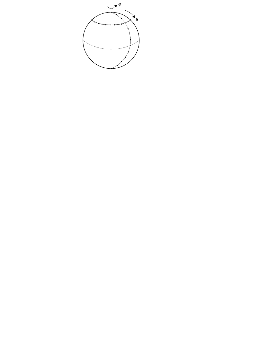
Figure 2: Discretization of a sphere.

where $b$ is a function of $\vartheta$ only. This models a surface of revolution (for example, a sphere as in Figure 2).

Using $B:={\rm diag}(1,b)$, we have $g=B^{t}B$ and the metric compatibility condition for the parallel transport takes the form

$$(BU_{\vartheta}\tilde{B}^{-1})^{t}\,(BU_{\vartheta}\tilde{B}^{-1})=I\;,\qquad(BU_{\varphi}B^{-1})^{t}\,(BU_{\varphi}B^{-1})=I$$ (6.6)

where $\tilde{B}:={\rm diag}(1,\tilde{b})$ and $\tilde{b}(\vartheta):=b(\vartheta+\ell)$. As a consequence of these equations, $\tilde{B}\,U_{\vartheta}\,B^{-1}$ and $B\,U_{\varphi}\,B^{-1}$ are elements of the orthogonal group $O(2)$. In order to obtain the correct continuum limit, we restrict them to be elements of $SO(2)$, the component of $O(2)$ which contains the identity. Then we have expressions

$$U_{\vartheta}=B^{-1}\,T(u)\,\tilde{B}\,,\qquad U_{\varphi}=B^{-1}\,T(v)\,B$$ (6.7)

where $u,v$ are arbitrary functions of $\vartheta$ and $\varphi$ and

$$T(\chi)=\left(\begin{array}[]{cc}\cos\chi&-\sin\chi\\ \sin\chi&\cos\chi\end{array}\right)\;.$$ (6.10)

The metric compatibility condition now leads to

$$U_{\vartheta}=\left(\begin{array}[]{cc}\cos u&-\tilde{b}\sin u\\ (1/b)\sin u&(\tilde{b}/b)\cos u\end{array}\right)\,,\qquad U_{\varphi}=\left(\begin{array}[]{cc}\cos v&-b\,\sin v\\ (1/b)\sin v&\cos v\end{array}\right)$$ (6.15)

and the condition of vanishing torsion becomes

$$\tilde{b}\sin u+\cos v=1\,,\qquad\tilde{b}\cos u-\sin v=b\;.$$ (6.16)

These equations determine $u$ and $v$ completely in terms of $b$ and $\tilde{b}$. We find

$$\cos u={1-p^{2}\over 1+p^{2}}\,,\;\sin u={2\,p\over 1+p^{2}}\,,\;\cos v={1+p^{2}-2\,\tilde{b}\,p\over 1+p^{2}}\,,\;\sin v={\tilde{b}-b-(\tilde{b}+b)\,p^{2}\over 1+p^{2}}$$ (6.17)

with

$$p=\left(2\,\tilde{b}\pm\sqrt{4\,\tilde{b}^{2}-(\tilde{b}^{2}-b^{2})^{2}}\right)/(b+\tilde{b})^{2}\;.$$ (6.18)

Only with the minus sign in the last expression we obtain a reasonable continuum limit, and this choice will be made in the following. The inverse parallel transport matrices are given by $V_{\vartheta}=\tilde{B}^{-1}T(-u)B$ and $V_{\varphi}=B^{-1}T(-v)B$, so that

$$V_{\vartheta}=\left(\begin{array}[]{cc}\cos u&b\sin u\\ -(1/\tilde{b})\sin u&(b/\tilde{b})\cos u\end{array}\right)\,,\qquad V_{\varphi}=\left(\begin{array}[]{cc}\cos v&b\sin v\\ -(1/b)\sin v&\cos v\end{array}\right)\;.$$ (6.23)

With $\lambda=\kappa^{-1}$ (see section 4), we obtain for the curvature

$$\lambda\circ\mathfrak{R}(\mbox{d}x^{\mu})=\sum_{\nu}r^{\mu}{}_{\nu}\,\mbox{d}\vartheta\,\mbox{d}\varphi\otimes_{L}\mbox{d}x^{\nu}$$ (6.24)

where $x^{1}=\vartheta,\,x^{2}=\varphi$ and

$$r := {1\over 2\ell^{2}}[U_{\vartheta}(\vartheta,\varphi)\,U_{\varphi}(\vartheta+\ell,\varphi)\,V_{\vartheta}(\vartheta,\varphi+\ell)\,V_{\varphi}(\vartheta,\varphi)$$ (6.27)

$$-U_{\varphi}(\vartheta,\varphi)\,U_{\vartheta}(\vartheta,\varphi+\ell)\,V_{\varphi}(\vartheta+\ell,\varphi)\,V_{\vartheta}(\vartheta,\varphi)]$$

$$= {1\over 2\ell^{2}}\,B^{-1}[T(u)\,T(\tilde{v})\,T(-u)\,T(-v)-T(v)\,T(u)\,T(-\tilde{v})\,T(-u)]\,B$$

$$= {1\over 2\ell^{2}}\,B^{-1}\,[T(\tilde{v}-v)-T(v-\tilde{v})]\,B$$

$$= {1\over\ell^{2}}\,\left(\begin{array}[]{cc}0&-b\,\sin(\tilde{v}-v)\\ (1/b)\sin(\tilde{v}-v)&0\end{array}\right)$$

with $\tilde{v}(\vartheta):=v(\vartheta+\ell)$. Since $u$ and $v$ are functions of $b$ and $\tilde{b}$, they are functions of $\vartheta$ only. Using

$$\mbox{d}\vartheta\,\mbox{d}\varphi=V^{\varphi}_{\vartheta\vartheta}\,\mbox{d}\vartheta\cap\mbox{d}\vartheta+V^{\varphi}_{\vartheta\varphi}\,\mbox{d}\vartheta\cap\mbox{d}\varphi\,,\quad\mbox{d}\varphi\,\mbox{d}\vartheta=V^{\vartheta}_{\varphi\vartheta}\,\mbox{d}\varphi\cap\mbox{d}\vartheta+V^{\vartheta}_{\varphi\varphi}\,\mbox{d}\vartheta\cap\mbox{d}\varphi$$ (6.28)

and $r\,\mbox{d}\vartheta\,\mbox{d}\varphi={1\over 2}\,r\,(\mbox{d}\vartheta\,\mbox{d}\varphi-\mbox{d}\varphi\,\mbox{d}\vartheta)$, we find the curvature components

$$\hat{R}_{\vartheta\vartheta}=-{\sin u\over\tilde{b}}\,r\,,\quad\hat{R}_{\vartheta\varphi}={b\,\cos u\over\tilde{b}}\,r\,,\quad\hat{R}_{\varphi\vartheta}=-(\cos v)\,r\,,\quad\hat{R}_{\varphi\varphi}=-b\,(\sin v)\,r$$ (6.29)

where $\hat{R}_{\kappa\lambda}=(\hat{R}^{\mu}{}_{\nu\kappa\lambda})$. We have the two Ricci tensors

$${\rm Ric} = {1\over\ell^{2}}\left(\begin{array}[]{cc}-(1/b)\cos v&-\sin v\\ (b/\tilde{b})\sin u&-(b^{2}/\tilde{b})\cos u\end{array}\right)\,\sin(\tilde{v}-v)$$ (6.32)

$$\overline{{\rm Ric}} = {1\over\ell^{2}}\left(\begin{array}[]{cc}(1/\tilde{b})\cos u&-\sin v\\ (b/\tilde{b})\sin u&b\,\cos v\end{array}\right)\,\sin(\tilde{v}-v)$$ (6.35)

and the combination

$$\widetilde{{\rm Ric}}:={1\over 2}({\rm Ric}-\overline{{\rm Ric}})=-{1\over 2\ell^{2}}({\cos u\over\tilde{b}}+{\cos v\over b})\,\sin(\tilde{v}-v)\;g$$ (6.36)

from which we obtain the curvature scalars

$$\hat{R} := g^{\mu\nu}\,{\rm Ric}_{\mu\nu}=-{1\over\ell^{2}}({\cos u\over\tilde{b}}+{\cos v\over b})\,\sin(\tilde{v}-v)$$ (6.37)

$$\bar{\hat{R}} := g^{\mu\nu}\,\overline{\rm Ric}_{\mu\nu}=-\hat{R}$$ (6.38)

$$\widetilde{R} := g^{\mu\nu}\,\widetilde{\rm Ric}_{\mu\nu}=\hat{R}\;.$$ (6.39)

Now (6.36) becomes

$$\widetilde{\rm Ric}_{\mu\nu}={1\over 2}\,\widetilde{R}\,g_{\mu\nu}\;.$$ (6.40)

These results clearly distinguish the particular linear combination (6.36) of Ricci tensors.

In the following, we present expansions in powers of $\ell$ and consider the continuum limit $\ell\to 0$. We shall allow an explicit dependence of $b$ on $\ell$, i.e., $b(\vartheta,\ell)=b_{0}(\vartheta)+b_{1}(\vartheta)\,\ell+{\cal O}(\ell^{2})$. Then

$$\Gamma_{\vartheta} = {1\over\ell}\,(U_{\vartheta}-I)$$ (6.45)

$$= \left(\begin{array}[]{cc}0&0\\ 0&b_{0}^{\prime}/b_{0}\end{array}\right)+\left(\begin{array}[]{cc}0&-(b_{0}^{\prime}{}^{2}/2)\\ b_{0}^{\prime}{}^{2}/2b_{0}^{2}&(2b_{1}^{\prime}+b_{0}^{\prime\prime})/2b_{0}-b_{1}b_{0}^{\prime}/b_{0}^{2}\end{array}\right)\,\ell+{\cal O}(\ell^{2})$$

$$\Gamma_{\varphi} = {1\over\ell}\,(U_{\varphi}-I)$$ (6.51)

$$= \left(\begin{array}[]{cc}0&-b_{0}b_{0}^{\prime}\\ b_{0}^{\prime}/b_{0}&0\end{array}\right)+\left(\begin{array}[]{cc}-b_{0}^{\prime}{}^{2}/2&-[b_{1}b_{0}^{\prime}+b_{0}b_{1}^{\prime}+b_{0}b_{0}^{\prime\prime}/2]\\ (2b_{1}^{\prime}+b_{0}^{\prime\prime})/2b_{0}-b_{1}b_{0}^{\prime}/b_{0}^{2}&-b_{0}^{\prime}{}^{2}/2\end{array}\right)\,\ell$$

$$+{\cal O}(\ell^{2})$$

where $b^{\prime}$ denotes the derivative of $b$ with respect to $\vartheta$. For the curvature, we find $\hat{R}_{\vartheta\vartheta}={\cal O}(\ell^{2})$ and

$$\hat{R}_{\vartheta\varphi} = \left(\begin{array}[]{cc}0&-b_{0}b_{0}^{\prime\prime}\\ b_{0}^{\prime\prime}/b_{0}&0\end{array}\right)$$

$$+\left(\begin{array}[]{cc}0&(-b_{1}+b_{0}^{\prime})\,b^{\prime\prime}_{0}-b_{0}\,(b_{1}^{\prime\prime}+b_{0}^{\prime\prime\prime})\\ -[(b_{1}+b_{0}^{\prime})b_{0}^{\prime\prime}/b_{0}^{2}-(b_{1}^{\prime\prime}+b_{0}^{\prime\prime\prime})/b_{0}]&0\end{array}\right)\,\ell$$

$$+{\cal O}(\ell^{2})$$

$$\hat{R}_{\varphi\vartheta} = \left(\begin{array}[]{cc}0&b_{0}\,b_{0}^{\prime}\\ -b_{0}^{\prime\prime}/b_{0}&0\end{array}\right)$$ (6.63)

$$+\left(\begin{array}[]{cc}0&b_{1}b_{0}^{\prime\prime}+b_{0}(b_{1}^{\prime\prime}+b_{0}^{\prime\prime\prime})\\ -[b_{1}b_{0}^{\prime\prime}-b_{0}(b_{1}^{\prime\prime}+b_{0}^{\prime\prime\prime})]/b_{0}^{2}&0\end{array}\right)\,\ell+{\cal O}(\ell^{2})$$

$$\hat{R}_{\varphi\varphi} = \left(\begin{array}[]{cc}0&b_{0}^{2}\,b_{0}^{\prime}\,b_{0}^{\prime\prime}\\ -b_{0}^{\prime}\,b_{0}^{\prime\prime}&0\end{array}\right)\,\ell+{\cal O}(\ell^{2})\;.$$ (6.66)

The Ricci tensors have the following expansions,

$${\rm Ric} = \left(\begin{array}[]{cc}-b_{0}^{\prime\prime}/b_{0}&0\\ 0&-b_{0}\,b_{0}^{\prime\prime}\end{array}\right)$$ (6.72)

$$+\left(\begin{array}[]{cc}[b_{1}b_{0}^{\prime\prime}-b_{0}(b_{1}^{\prime\prime}+b_{0}^{\prime\prime\prime})]/b_{0}^{2}&-b_{0}^{\prime}\,b_{0}^{\prime\prime}\\ 0&(-b_{1}+b_{0}^{\prime})\,b_{0}^{\prime\prime}-b_{0}\,(b_{1}^{\prime\prime}+b_{0}^{\prime\prime\prime})\end{array}\right)\,\ell+{\cal O}(\ell^{2})\qquad$$

$$\overline{\rm Ric} = \left(\begin{array}[]{cc}b_{0}^{\prime\prime}/b_{0}&0\\ 0&b_{0}\,b_{0}^{\prime\prime}\end{array}\right)$$ (6.78)

$$+\left(\begin{array}[]{cc}-(b_{1}+b_{0}^{\prime})\,b_{0}^{\prime\prime}/b_{0}^{2}+(b_{1}^{\prime\prime}+b_{0}^{\prime\prime})/b_{0}&-b_{0}^{\prime}\,b_{0}^{\prime\prime}\\ 0&b_{1}\,b_{0}^{\prime\prime}+b_{0}\,(b_{1}^{\prime\prime}+b_{0}^{\prime\prime\prime})\end{array}\right)\,\ell+{\cal O}(\ell^{2})\qquad$$

$$\widetilde{\rm Ric} = \left[-{b_{0}^{\prime\prime}\over b_{0}}+{2b_{1}b_{0}^{\prime\prime}+b_{0}^{\prime}b_{0}^{\prime\prime}-2b_{0}(b_{1}^{\prime\prime}+b_{0}^{\prime\prime\prime})\over 2b_{0}^{2}}+{\cal O}(\ell^{2})\right]\,g_{0}$$ (6.79)

where $g_{0}:=\mbox{diag}(1,b_{0}^{2})$. For the curvature scalar we obtain

$$\hat{R}=-{2b_{0}^{\prime\prime}\over b_{0}}+{2b_{1}b_{0}^{\prime\prime}+b_{0}^{\prime}b_{0}^{\prime\prime}-2b_{0}(b_{1}^{\prime\prime}+b_{0}^{\prime\prime\prime})\over b_{0}^{2}}+{\cal O}(\ell^{2})$$ (6.80)

Example. In ordinary continuum differential geometry, the standard geometry of the unit sphere is obtained with $b(\vartheta)=\sin\vartheta$. With this choice, we get

$$\hat{R}=2+\ell\,\mbox{cot}\,\vartheta+{\cal O}(\ell^{2})\;.$$ (6.81)

in the discrete framework and in the limit $\ell\to 0$ we recover the continuum result $\hat{R}=2$. To first order, there is a dependence of the curvature scalar on $\vartheta$. With the refined choice $b(\vartheta,\ell)=[1+\vartheta\ell/4+{\cal O}(\ell^{2})]\,\sin\vartheta$, we get

$$\hat{R}=2+{\cal O}(\ell^{2})\;.$$ (6.82)

$\blacksquare$

Our discrete version of curvature describes finite distances on a space in contrast to infinitesimal distances as expressed by tangent vectors in continuum differential geometry. This means that the metric components in the case under consideration have to be expected to depend on the discretization (which should be regarded as a discretization of a chart), i.e., on $\ell$ in the case under consideration. We still have to understand how, for example, spherical symmetry can be formulated in our framework. Then, we should be able to determine a spherically symmetric metric as a suitable discrete counterpart of the Riemannian metric of the (continuum) sphere. Furthermore, it remains to be seen how this is related to the metric with constant curvature scalar, approximated in the above example.

7 Conclusions

Within a framework of noncommutative geometry, we have presented a formalism of discrete Riemannian geometry which is very much analogous to continuum Riemannian geometry.

Whereas the general formalism of noncommutative geometry suggests to consider a (generalized) metric tensor as an element of $\Omega^{1}\otimes_{\cal A}\Omega^{1}$, in this paper it was taken to be an element of $\Omega^{1}\otimes_{L}\Omega^{1}$ since a simple geometric meaning can be assigned to its components (with respect to the canonical basis $e^{ij}$ of $\Omega^{1}$, cf section 3).

The compatibility condition $\nabla g=0$ for a metric and a linear connection on a finite set, when expressed in terms of parallel transport matrices, leads to relations (cf section 3.5) which are in complete accordance with what one should expect on the basis of a reformulation of metric compatibility in terms of parallel transport in (continuum) differential geometry.

An important role in ordinary differential geometry and especially in General Relativity is played by the Ricci tensor and the curvature scalar. There is no generalization of these tensors to the general framework of noncommutative geometry. In the case of a discrete set, we considered this problem in some detail in section 4 and showed that, with certain restrictions on the differential calculus (and thus the links between the points of the set), satisfactory candidates for discrete counterparts of the continuum Ricci tensor and curvature scalar do exist. The examples treated in sections 4-6 demonstrate how our definitions work. It should be quite evident by now that general definitions can hardly be expected since in noncommutative geometry, and already with a commutative algebra ${\cal A}$, we are dealing with a huge variety of structures of which only few should be expected to be close (in some sense) to continuum differential geometry.

In the last two sections we have developed discrete differential geometry on a hypercubic lattice. Since we were able to construct a Ricci tensor and a curvature scalar in this case, discrete counterparts of the (vacuum) Einstein equations are obtained. The results of the last section suggest to choose the following version,

$$\widetilde{\rm Ric}_{\mu\nu}-{1\over 2}\,\widetilde{R}\,g_{\mu\nu}=0\;.$$ (7.1)

On the left hand side we have tensor components in the sense that they transform covariantly under a change of module basis in the space of 1-forms. It is straightforward to include matter fields in this scheme. The ‘discrete gravity’ theory which we propose here is very different from earlier approaches which were either based on Regge calculus [19], other simplicial complex structures [20], or on a certain reformulation of gravity as a gauge theory [21]. The correspondence between first order differential calculi on discrete sets and digraphs relates our formalism to the spin network approach to (quantum) gravity (see [22], in particular) at least on a basic level.

Acknowledgments. A D is grateful to Professor Theo Geisel for financial support during a stay at the Max-Planck-Institut für Strömungsforschung. F M-H would like to thank John Madore for a discussion.

References

• [1] A. Dimakis and F. Müller-Hoissen, “Quantum mechanics on a lattice and $q$-deformations”, Phys. Lett. B 295, 242 (1992).
• [2] A. Dimakis and F. Müller-Hoissen, “Differential calculus and gauge theory on finite sets”, J. Phys. A 27, 3159 (1994).
• [3] A. Dimakis and F. Müller-Hoissen, “Discrete differential calculus, graphs, topologies and gauge theory”, J. Math. Phys. 35, 6703 (1994).
• [4] A. Dimakis, F. Müller-Hoissen and F. Vanderseypen, “Discrete differential manifolds and dynamics on networks”, J. Math. Phys. 36, 3771 (1995).
• [5] K. Bresser, A. Dimakis, F. Müller-Hoissen and A. Sitarz, “Non-commutative geometry of finite groups”, J. Phys. A 29, 2705 (1996).
• [6] A. Dimakis, F. Müller-Hoissen and T. Striker, “Noncommutative differential calculus and lattice gauge theory”, J. Phys. A 26, 1927 (1993).
• [7] A. Dimakis and F. Müller-Hoissen, “Integrable discretizations of chiral models via deformation of the differential calculus”, J. Phys. A 29, 5007 (1996).
• [8] A. Connes, Noncommutative Geometry (Academic Press, San Diego, 1994).
• [9] A. Dimakis and F. Müller-Hoissen, “Connes’ distance function on one-dimensional lattices”, Int. J. Theor. Phys. 37, 907 (1998).
• [10] A. Sitarz, “Gravity from noncommutative geometry”, Class. Quantum Grav. 11, 2127 (1994); “On some aspects of linear connections in noncommutative geometry”, preprint hep-th/9503103.
• [11] M. Dubois-Violette, J. Madore, T. Masson and J. Mourad, “Linear connections on the quantum plane”, Lett. Math. Phys. 35, 351 (1995).
• [12] I. Heckenberger and K. Schmüdgen, “Levi-Civita connections on the quantum groups $SL_{q}(N)$, $O_{q}(N)$ and $Sp_{q}(N)$”, q-alg/9512001.
• [13] A. Dimakis, “A note on connections and bimodules”, q-alg/9603001.
• [14] A. Dimakis and F. Müller-Hoissen, “Deformations of classical geometries and integrable systems”, preprint physics/9712002.
• [15] S. Cho and K.S. Park, “Linear connections on graphs”, J. Math. Phys. 38, 5889 (1997).
• [16] R.R. Zapatrin, “Polyhedral representations of discrete differential manifolds”, J. Math. Phys. 38, 2741 (1997).
• [17] H.C. Baehr, A. Dimakis and F. Müller-Hoissen, “Differential calculi on commutative algebras”, J. Phys. A 28, 3197 (1995).
• [18] L. Brewin, “Riemann normal coordinates, smooth lattices and numerical relativity”, gr-qc/9701057.
• [19] T. Regge, “General relativity without coordinates”, Nuovo Cim. A 19, 558 (1961); R.M. Williams and P.A. Tuckey, “Regge calculus: a brief review and bibliography”, Class. Quantum Grav. 9, 1409 (1992).
• [20] D. Weingarten, “Geometric formulation of electrodynamics and general relativity in discrete space-time”, J. Math. Phys. 18, 165 (1977);
A. N. Jourjine, “Discrete gravity without coordinates”, Phys. Rev. D35, 2983 (1987).
• [21] A. Das, M. Kaku and P.K. Townsend, “Lattice formulation of general relativity”, Phys. Lett. B 81, 11 (1979);
L. Smolin, “Quantum gravity on a lattice”, Nucl. Phys. B 148, 333 (1979);
K.I. Macrea, “Rotationally invariant field theory on lattices. III. Quantizing gravity by means of lattices”, Phys. Rev. D23 900 (1981);
C.L.T. Mannion and J.G. Taylor, “General relativity on a flat lattice”, Phys. Lett. B 100, 261 (1981);
K. Kondo, “Euclidean quantum gravity on a flat lattice”, Progr. Theor. Phys. 72, 841 (1984);
M. Caselle, A. D’Adda and L. Magnea, “Lattice gravity and supergravity as spontaneously broken gauge theories of the (super) Poincaré group”, Phys. Lett. B 192, 406 (1987), “Doubling of all matter fields coupled to gravity on a lattice”, Phys. Lett. B 192, 411 (1987);
P. Renteln and L. Smolin, “A lattice approach to spinorial quantum gravity”, Class. Quantum Grav. 6, 275 (1989);
O. Boström, M. Miller and L. Smolin, “A new discretization of classical and quantum general relativity”, preprint CGPG 94-3-3;
R. Loll, “Discrete approaches to quantum gravity in four dimensions”, gr-qc/9805049.
• [22] A. Ashtekar and J. Lewandowski, “Quantum theory of geometry I: area operators”, Class. Quantum Grav. 14, A55 (1997);
F. Markopoulou and L. Smolin, “Causal evolution of spin networks”, Nucl.Phys. B 508, 409 (1997);
M.P. Reisenberger, “A lattice worldsheet sum for 4-d Euclidean general relativity”, gr-qc/9711052.