Abstract

In the path integral approach to false vacuum decay with the effect of gravity, there is an unsolved problem, called the negative mode problem. We show that the appearance of a supercritical supercurvature mode in the one-bubble open inflation scenario is equivalent to the existence of a negative mode around the Euclidean bounce solution. Supercritical supercurvature modes are those whose mode functions diverge exponentially for large spatial radius on the time constant hypersurface of the open universe. Then we propose a conjecture that there should be “no supercritical supercurvature mode”. For a class of models that contains a wide variety of tunneling potentials, this conjecture is shown to be correct.

I introduction

The Euclidean path integral approach has been used to investigate the true vacuum bubble nucleation through quantum tunneling[1, 2]. In the lowest WKB approximation, the quantum tunneling is described by a bounce solution. The bounce solution is a solution of the Euclidean equation of motion, which connects the configurations before and after tunneling. The bounce solution that takes account of the gravitational effect was found by Coleman and De Luccia[3].

The decay rate per unit volume and per unit time interval, $\Gamma$, is given by the formula[1]

$$\Gamma=|K|e^{-(S_{E}^{(bounce)}-S_{E}^{(trivial)})},$$ (1)

where $S_{E}^{(bounce)}$ is the classical Euclidean action for the bounce solution and $S_{E}^{(trivial)}$ is that for the trivial solution that stays at the false vacuum. In the path integral approach, the prefactor $|K|$ is evaluated by the gaussian integral over fluctuations around the background bounce solution. In a standard system which does not take account of gravity, there is one perturbation mode in which direction the action decreases. It is called a negative mode. For this mode, the gaussian integral is not well-defined. To make the integral finite, the integration path should be deformed on the complex plane. Consequently, one imaginary factor, $i$, appears in $K$. In the Euclidean path integral approach to tunneling, this imaginary unit plays a crucial role to interpret $\Gamma$ as the decay rate.

However, in the case when gravity is taken into account, the situation changes drastically. Since there are gauge degrees of freedom, we have various possibilities in choosing variables to describe the physical degrees of freedom. If we choose inappropriate variables, the equation that determines the fluctuation mode can become singular. In Ref.[4], we have shown that it is impossible to obtain a well-behaved reduced action as long as we stick to variables that appear in the original Lagrangian in the second order formalism. In order to find variables that can lead us to a well-behaved reduced action, it was necessary to resort to the Hamiltonian formalism. In the Hamiltonian formalism, conjugate momenta are introduced, and hence wider varieties of choice of variables are allowed. In Ref.[4], we derived a well-behaved reduced action for fluctuations around the $O(4)$-symmetric bounce solution. We found the action for fluctuations which conserve the $O(4)$-symmetry has an unusual signature. Namely the kinetic term is negative definite. To deal with this action, we proposed a prescription analogous to the conformal rotation[5]. Then, from the path integral measure, there arises one imaginary unit $i$. This suggests there should be no negative mode in the final form of the reduced action, since the factor $i$ in $K$ has been already taken care of by the above mentioned prescription. Therefore, we proposed the “no negative mode conjecture”[4].

On the other hand, in recent years the process of false vacuum decay with the effect of gravity has been studied extensively in the context of the one-bubble open inflation scenario. In this scenario, an open universe is created inside a nucleated bubble. In one-bubble open inflation, one of the most important issues is to calculate the spectrum of quantum fluctuations after the bubble nucleation because it determines the spectrum of cosmological perturbations. By comparing the predicted spectrum with the observed one, we can test a model of one-bubble open inflation.

Fluctuations in an open universe can be decomposed by using spatial harmonics on the unit 3-dimensional hyperbolic space. We denote the eigenvalue of a spatial harmonic by $-(p^{2}+1)$. The spatial harmonics with positive $p^{2}$ are square-integrable functions on a time constant hypersurface in an open universe in the sense that they can be normalized by using the Dirac delta function. As a result the spectrum is continuous for $p^{2}>0$. On the other hand, the spatial harmonics are no longer square-integrable for $p^{2}<0$. However, since a time constant hypersurface in an open universe is not a Cauchy surface, this divergence does not directly exclude such modes. By considering the normalization of perturbation modes on a Cauchy surface, we find that the spectrum for $p^{2}<0$ becomes discrete. These modes are called supercurvature modes since they give rise to correlation on scales greater than the spatial curvature scale[6, 7].

There are two classes of supercurvature modes, which we call supercritical and subcritical modes. The precise definition will be presented later. Here we mention that supercritical modes have smaller values (i.e., larger absolute values) of $p^{2}$ than subcritical modes, and their mode functions diverge exponentially for large spatial radius in the open universe. We shall show that the existence of a supercritical supercurvature mode is equivalent to the existence of a negative mode. Thus the “no negative mode conjecture” presented in Ref.[4] can be restated as the “no supercritical supercurvature mode conjecture”. Note that there exists no supercurvature mode for a model with sufficiently thin bubble wall[8], hence there is no supercritical mode in such a model. The purpose of this paper is to examine this conjecture for a wider class of models. In particular, a class of models we consider naturally allows thick bubble wall solutions. Recently the negative mode problem has been discussed by Lavrelashvili[9] in the context of the singular Hawking-Turok instanton[10]. In this paper, however, we exclude the possibility of the Hawking-Turok instanton and focus on regular bounce solutions.

In section 2, we show the equivalence between the existence of a negative mode in the reduced Euclidean action and that of a supercritical supercurvature mode in the spectrum of cosmological perturbations. In section 3, we give a method to construct potential models which allow an analytical treatment. By using this method, we give a set of models which seemingly violate our conjecture. In section 4, for such models that have a bounce solution with a negative mode, we show that there should be another bounce solution that has a smaller value of the action and has no negative mode. Conclusion is given in section 5.

II negative mode and supercritical supercurvature mode

We consider a system composed of a real scalar field, $\Phi$, coupled with the Einstein gravity. The Euclidean action is given by

$$S_{E}=\int d^{4}x\,\sqrt{g}\left[-{1\over 2\kappa}R+{1\over 2}g^{\mu\nu}\partial_{\mu}\Phi\partial_{\nu}\Phi+V(\Phi)\right].$$ (2)

The potential of the scalar field is assumed to have the form as shown in Fig. 1, and initially the field is assumed to be trapped in the false vacuum. As mentioned in Introduction, the bounce solution is a Euclidean solution that connects the configurations before and after tunneling. In the present case, the geometry before false vacuum decay is given by a de Sitter space. After tunneling, there appears a true vacuum bubble in the false vacuum sea. This bounce solution is obtained by Coleman and De Luccia[3] under the assumption of the $O(4)$-symmetry:

$$ds^{2}=a^{2}(\eta)\left\{d\eta^{2}+d\chi^{2}+\sin^{2}\chi\,d\Omega_{(2)}^{2}\right\},\quad\Phi=\phi(\eta).$$ (3)

The Euclidean equations of motion are

$$\phi^{\prime\prime}+2{\cal H}\phi^{\prime}-a^{2}{dV(\phi)\over d\phi}=0,$$ (4)

$${\cal H}^{2}-1={\kappa\over 3}\left({1\over 2}{\phi^{\prime}}^{2}-a^{2}V(\phi)\right),$$ (5)

$${\cal H}^{\prime}-{\cal H}^{2}+1=-{\kappa\over 2}{\phi^{\prime}}^{2},$$ (6)

where a prime represents the differentiation with respect to $\eta$ and ${\cal H}:=a^{\prime}/a$. Requiring the regularity of the bounce solution, the boundary condition is determined as

$$\phi^{\prime}\propto e^{-2|\eta|},\quad a\propto e^{-|\eta|},\quad(\eta\to\mp\infty).$$ (7)

By choosing the initial value of $\phi$ at $\eta\to-\infty$ appropriately, we obtain a solution which satisfies the required boundary condition. For definiteness, we choose $\phi$ to be in the false vacuum side for $\eta\to-\infty$.

FIG. 1.: A typical shape of a scalar field potential under consideration.

As noted before, the number of $i$’s in the prefactor $K$ has a crucial meaning in the path integral approach. To evaluate this number, we need to derive the reduced action for fluctuations around the bounce solution. The fluctuations can be expanded in terms of the spherical harmonics on the unit 3-sphere, say $Y_{n\ell m}$ with $n=0$, $1$, $2$, $\cdots$, which satisfy $\bigl{[}{}^{(3)}\Delta+n(n+2)\bigr{]}Y_{n\ell m}=0$. After appropriate gauge fixing, we obtain[4, 11]

$$\delta^{(2)}S=\sum_{n\ell m}{(n+3)(n-1)\over 2}\int d\eta\left[-i\pi^{n\ell m}{dq^{n\ell m}\over d\eta}+{1\over 2}|\pi^{n\ell m}|^{2}+{1\over 2}(U+(n+3)(n-1))|q^{n\ell m}|^{2}\right],$$ (8)

where $q^{n\ell m}$ is the coefficient of the harmonic expansion of a gauge-invariant variable $q$, and $\pi^{n\ell m}$ its conjugate. In our original derivation[4], we used the variable $h:=q/a$ and its conjugate momentum. The variable $q$ is equal to the Euclidean version of $\textstyle q$ introduced in Ref.[11]. Here, the potential $U$ is given by

$$U={\kappa\over 2}\phi^{\prime}{}^{2}-W^{\prime}+W^{2}\;\quad W={\phi^{\prime\prime}\over\phi^{\prime}}\,.$$ (9)

Physically, the variable $q$ represents the curvature perturbation in the Newton gauge when analytically continued to the open universe inside the bubble. The explicit form of the perturbation in this gauge is

$$ds^{2}= a^{2}\left[\left(1+{\kappa\phi^{\prime}q\over a}\right)d\eta^{2}+\left(1-{\kappa\phi^{\prime}q\over a}\right)\left(d\chi^{2}+\sin^{2}\chi d\Omega_{(2)}^{2}\right)\right],$$ (10)

$$\varphi:= \Phi-\phi={1\over\phi^{\prime}}{d\over d\eta}(\phi^{\prime}q),$$ (11)

where $\varphi$ is the perturbation of the scalar field. Recall that the prefactor $K$ is evaluated as[1]

$$K=\int[d\pi\,dq]e^{-\delta^{(2)}S}.$$ (12)

Looking at Eq. (8), we find that the action disappears for $n=1$. This just reflects the fact that the $n=1$ modes are pure gauge and there is no physical degree of freedom in them. This is very different from the case of false vacuum decay in the flat spacetime, in which there is a zero mode in the $n=1$ modes. This zero mode describes spacetime translation modes and its existence implies the existence of a unique negative mode in the $n=0$ (i.e., $O(4)$ symmetric) modes[12]. In the present case of false vacuum decay with gravity, the coefficient in front of $|\pi^{n\ell m}|^{2}$ becomes negative for $n=0$. Therefore if we try to perform the integration with respect to $\pi$, we find that the gaussian integral does not converge for $n=0$. To resolve this difficulty, we proposed in [4] a prescription analogous to the conformal rotation. By changing the variables as $\pi\to-i\pi$, $q\to iq$, the above path integral becomes well-defined. To carry out the path integral, the variables must be discretized. Then the numbers of $p$ and $q$ integrals will differ by 1. Therefore, this change of variables will produce one imaginary unit $i$ for the prefactor $K$. This is in contrast to the case of false vacuum decay in the flat spacetime in which the imaginary unit $i$ in $K$ arises from the negative mode. Note that there is no negative mode for $n\geq 2$[9].

Let us examine the $n=0$ case in more detail. If we know the spectrum of eigenvalues, $\lambda_{j}$, of the following Shrödinger-type equation,

$$\left(-{d^{2}\over d\eta^{2}}+U-3\right)q_{j}=\lambda_{j}q_{j},$$ (13)

where $q_{j}$ is the $j$-th eigenfunction, the contribution to $K$ from $n=0$ modes, will be given by $\sim(-i)\prod\lambda_{j}^{-1/2}$, where the factor $(-i)$ comes from the rotation of the variables as explained above. If there is a mode with a negative eigenvalue, there arises another imaginary factor, and hence the prefactor $K$ becomes real. If so, this bounce solution will not contribute to the tunneling process in the path integral approach. On the other hand, there is another approach to describe the tunneling. That is the approach to construct a WKB wave function[13, 4]. In this approach, any bounce solution that connects false and true vacua will contribute to the tunneling, putting aside the issue of which bounce dominates. Thus, in order that the consistency is kept between the path integral approach and the wave function approach, there should be no negative mode for the Coleman-De Luccia bounce solution, provided it gives the smallest Euclidean action among the non-trivial bounce solutions. This is the conjecture proposed in Ref.[4].

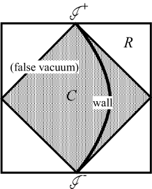
FIG. 2.: Conformal diagram of a de Sitter-like space with a bubble wall. The Cauchy surface exists in region $C$ but not in the open universe inside bubble, the region marked as $R$.

Now, let us turn to the problem of the perturbation spectrum in the context of the one-bubble open inflation scenario. To study it, we need to quantize the perturbation field on the non-trivial background that appears after tunneling. For this purpose, the reduced action for the perturbation field must be calculated. In doing so, the time coordinate must be chosen so that the time constant hypersurface is a Cauchy surface. A convenient choice is to use the coordinate that is obtained by the analytic continuation of $\chi$: $\chi_{c}=i(\chi-\pi/2)$. Then, the coordinates $(\chi_{c},\eta,\Omega_{(2)})$ span the region $C$ of Fig. 2. In region $C$, the metric takes the form

$$ds^{2}=a^{2}(\eta)\left(d\eta^{2}-d\chi_{c}^{2}+\cosh^{2}\chi_{c}\,d\Omega_{(2)}^{2}\right).$$ (14)

It should be remembered that $\eta$ is not a time coordinate there. The reduced action in this region is obtained as

$$S^{(2)}=\sum_{\ell,m}{1\over 2}\int d\chi_{c}\int{d\eta}\left[\cosh^{2}\chi_{c}{\partial\overline{{\mathchoice{{\hbox{\boldmath$\displaystyle q$}}}{{\hbox{\boldmath$\textstyle q$}}}{{\hbox{\boldmath$\scriptstyle q$}}}{{\hbox{\boldmath$\scriptscriptstyle q$}}}}^{\ell m}}\over\partial\chi_{c}}\hat{\cal O}{\partial{\mathchoice{{\hbox{\boldmath$\displaystyle q$}}}{{\hbox{\boldmath$\textstyle q$}}}{{\hbox{\boldmath$\scriptstyle q$}}}{{\hbox{\boldmath$\scriptscriptstyle q$}}}}^{\ell m}\over\partial\chi_{c}}-\overline{{\mathchoice{{\hbox{\boldmath$\displaystyle q$}}}{{\hbox{\boldmath$\textstyle q$}}}{{\hbox{\boldmath$\scriptstyle q$}}}{{\hbox{\boldmath$\scriptscriptstyle q$}}}}^{\ell m}}\hat{\cal O}\left\{{\ell(\ell+1)}+(\hat{\cal O}-3)\cosh^{2}\chi_{c}\right\}{\mathchoice{{\hbox{\boldmath$\displaystyle q$}}}{{\hbox{\boldmath$\textstyle q$}}}{{\hbox{\boldmath$\scriptstyle q$}}}{{\hbox{\boldmath$\scriptscriptstyle q$}}}}^{\ell m}\right],$$ (15)

where $\hat{\cal O}$ is defined by

$$\hat{\cal O}:=-{\partial^{2}\over\partial\eta^{2}}+U,$$ (16)

and $U$ is the same as the one given in Eq.(9). In this expression, the $\eta$-dependence appears only through the operator $\hat{O}$. Thus the perturbation can be expanded by using eigenfunctions of $\hat{O}$: ${\mathchoice{{\hbox{\boldmath$\displaystyle q$}}}{{\hbox{\boldmath$\textstyle q$}}}{{\hbox{\boldmath$\scriptstyle q$}}}{{\hbox{\boldmath$\scriptscriptstyle q$}}}}^{\ell m}=\sum_{p}q^{p}(\eta)f^{p\ell m}(\chi_{c})$. The equation that determines eigenvalues and eigenfunctions is

$$\left[-{d^{2}\over d\eta^{2}}+U\right]q^{p}=(p^{2}+4)q^{p}.$$ (17)

Analyzing the asymptotic behavior of $\phi$, we find $U\to 4$ for $\eta\to\mp\infty$. Hence the spectrum is continuous for $p^{2}>0$. On the other hand, the spectrum for $p^{2}<0$ is discrete, which are called supercurvature modes. Here we call modes with $p^{2}<-1$ supercritical supercurvature, while we call modes with $0>p^{2}>-1$ subcritical supercurvature. When analytically continued to the open universe by $\chi_{R}=\chi_{c}+i\pi/2$, the supercritical modes diverge exponentially for $\chi_{R}\to\infty$. By comparing Eqs. (13) and (17), the existence of a negative mode around the bounce solution is manifestly equivalent to that of a supercritical supercurvature mode in the spectrum of quantum fluctuations in the open universe. Thus the conjecture that we stated above can be restated as the “no supercritical supercurvature mode conjecture”.

III model construction

At first sight, there seems no reason to deny the possibility of a potential model that allows a bounce solution with a supercritical supercurvature mode. In fact, there is a method to construct such models, as described in a separate paper[8]. However, as mentioned there, this method does not guarantee that thus obtained bounce solution gives the smallest Euclidean action among non-trivial solutions. Hence, given a bounce solution that allows a supercritical supercurvature mode, if one can prove that its action is not the smallest, our conjecture remains intact.

In this section, we review the method to construct a potential model and a bounce solution, and give an example in which a supercritical supercurvature mode appears when a model parameter is varied. We then construct a potential model that allows a continuous series of bounce solutions under the weak gravitational backreaction approximation, which will be used for the investigation of the negative mode problem in the next section.

Our method for model construction is as follows. We first give $\phi^{\prime}$. It can be specified rather arbitrarily except for the conditions that it vanishes as $e^{-2|\eta|}$ for $\eta\to\mp\infty$ and it is positive (or negative) definite so that $\phi$ is a monotonic function of $\eta$. Then we solve the equations (6) to find ${\cal H}$ and $a$. For $\eta\to\mp\infty$, ${\cal H}$ is solved as

$${{\cal H}-1\over{\cal H}+1}=C_{\mp}e^{2\eta}\,.$$

Thus the required boundary condition, ${\cal H}\to\pm 1$ for $\eta\to\mp\infty$, is automatically satisfied. Once we know ${\cal H}$, we can determine $a$ by integrating ${\cal H}$. Here an integration constant appears, which determines the absolute value of the potential, say the potential at the false vacuum $V_{F}$. Finally, using Eq. (5), the potential $V$ is determined as a function of $\eta$ as

$$V(\phi(\eta))={6-6{\cal H}^{2}+{\kappa}{\phi^{\prime}}^{2}\over 2\kappa a^{2}}\,.$$ (18)

By assumption, since $\phi$ is a monotonic function of $\eta$, by inversely expressing $\eta$ in terms of $\phi$, the shape of the potential is uniquely determined.

Next we turn to the eigenvalue equation (13). If there is a negative mode, the solution with $\lambda=0$ must have, at least, one node. Hence, it is sufficient to examine the equation for ${\lambda=0}$, which is written as

$$\left[-{d^{2}\over d\eta^{2}}+{\kappa\over 2}{\phi^{\prime}}^{2}-W^{\prime}+W^{2}-3\right]q=0.$$ (19)

If the second term, $\kappa\phi^{\prime}{}^{2}/2$ is large enough, the potential will stay positive and hence $q$ will have no node. Since the change in the overall amplitude of $\phi^{\prime}$ does not alter the function $W$, we can construct a model in which the second term is negligibly small without changing the other terms. Hence, we neglect this positive definite term for the moment.

From the boundary condition, we find that $W$ behaves as

$$W\to\pm 2,\quad(\eta\to\mp\infty).$$

Except for this boundary condition, $W$ can be arbitrarily chosen. Then, by choosing $W$ to stay close to zero for a sufficiently long interval of $\eta$, the potential term, $-W^{\prime}+W^{2}-3$, will have a wide negative-valued region, and the solution for $q$ will have a node. In contrast, if we consider a sufficiently thin wall, the $W^{\prime}$ term will dominate the potential when $|W|$ is small and $W^{\prime}<0$. Then, the potential will stay positive, and hence $q$ has no node[8].

For instance, let us consider a set of models in which $W$ is given by

$$W=-2\tanh((\eta-\zeta)/\Delta),$$ (20)

where the model parameters $\zeta$ and $\Delta$ represent the wall location and its thickness, respectively. This is realized by setting

$$\phi^{\prime}={\mu\over\left(\cosh((\eta-\zeta)/\Delta)\right)^{2\Delta}}\,,$$ (21)

where $\mu$ is a constant. Then, neglecting the $\kappa\phi^{\prime}{}^{2}/2$ term, Eq. (19) becomes

$$\left[-{d^{2}\over d\eta^{2}}+\left({2\over\Delta}-4\right){1\over\cosh^{2}((\eta-\zeta)/\Delta)}+1\right]q=0.$$ (22)

For $\Delta=1$, this equation has a regular nodeless solution,

$$q={1\over\cosh(\eta-\zeta)}\,.$$ (23)

Thus the lowest eigenvalue is zero for $\Delta=1$. Since the potential term in Eq. (22) is a monotonically decreasing function of $\Delta$, there will be a negative mode for $\Delta>1$. Now let us turn on the $\kappa\phi^{\prime}{}^{2}/2$ term while keeping $W$ the same. As we increase $\mu$, the critical value of $\Delta$ for the existence of a negative mode will increase. For $\kappa\mu^{2}\gtrsim 1$, a negative mode will disappear completely for any value of $\Delta$.

To make the problem tractable, let us consider the weak backreaction limit, in which the geometry can be approximated by a pure de Sitter space. From Eq. (6), we see that this will be the case if $\kappa\phi^{\prime}{}^{2}\ll 1$. In the above model, we have seen that a negative mode will disappear if the $\kappa\phi^{\prime}{}^{2}/2$ term gives a large contribution (of order unity or greater) to the potential. This will be true for most conceivable potential models. Hence we may restrict our attention to a class of models that automatically satisfy the weak backreaction condition when investigating the existence of a negative mode.

In the first non-trivial order of the weak backreaction approximation, we find that the negative mode problem can be analyzed on a fixed de Sitter background geometry. Let us explicitly show this fact.

First we examine the background field equations. Neglecting relative errors of $O(\kappa\phi^{\prime}{}^{2})$, Eq. (6) can be readily solved as

$$a_{b}={1\over H\cosh\eta}\,,\quad{\cal H}_{b}=-\tanh\eta\,,$$ (24)

where $H$ is defined by $H^{2}:=(\kappa/3)V_{top}$ where $V_{top}$ is the value of $V$ at the top of the potential barrier. It is worthwhile to note that the weak backreaction approximation does not imply small potential difference between the false and true vacua. The vacuum energy inside the bubble can be much smaller than $V_{F}$ as long as the bubble radius is sufficiently smaller than $H^{-1}$. However, the weak backreaction approximation does imply $V_{top}-V_{F}\ll V_{F}$. Hence we may replace $V_{top}$ with $V_{F}$ in the definition of $H$. Here we have chosen $V_{top}$ for later convenience. Then substituting the lowest order solutions of $a$ and ${\cal H}$ to Eq. (4), the scalar field equation becomes

$$\phi^{\prime\prime}+2{\cal H}_{b}\phi^{\prime}-a_{b}^{2}{d\over d\phi}(\delta V)=0,$$ (25)

where $\delta V=V-V_{top}$. This gives the lowest order solution of $\phi$. Introducing the variable $N:=\log a$, and expanding it as $N_{b}+\delta N$, Eq. (6) gives the equation for the first order correction to $a$:

$${1\over\cosh^{2}\eta}{d\over d\eta}\left(\cosh^{2}\eta\,{d(\delta N)\over d\eta}\right)=-{\kappa\over 2}\phi^{\prime}{}^{2}.$$ (26)

Since $\phi^{\prime}{}^{2}\sim e^{-4|\eta|}$ for $\eta\to\pm\infty$, the above equation can be integrated and we find $\delta N=O(\kappa\phi^{\prime}{}^{2})$ everywhere. If we substitute this $\delta N$ back into Eq. (4), we can calculate the correction of $O(\kappa\phi^{\prime}{}^{2})$ to $\phi$.

Next we evaluate the action under the weak backreaction approximation. The Euclidean action for an $O(4)$-symmetric configuration is given by

$$S_{E}= S_{g}[a]+S_{m}[a,\phi];$$ (29)

$$S_{g}[a]:=2\pi^{2}\int d\eta\left[-{3\over\kappa}a^{\prime}{}^{2}-{3\over\kappa}a^{2}+a^{4}V_{top}\right],$$

$$S_{m}[a,\phi]:=2\pi^{2}\int d\eta\left[{a^{2}\over 2}\phi^{\prime}{}^{2}+a^{4}\delta V(\phi)\right].$$

Inserting $a_{b}+\delta a$ to the gravitational part of the action, where $\delta a=a_{b}\delta N=O(\kappa\phi^{\prime}{}^{2})$, we find

$$S_{g}[a_{b}+\delta a]=S_{g}[a_{b}]\left(1+O\left((\kappa\phi^{\prime}{}^{2})^{2}\right)\right),$$ (30)

which follows from the fact that $a_{b}$ is a solution to the equation obtained from the action $S_{g}[a]$. Hence, to the first order of $\kappa\phi^{\prime}{}^{2}$, we have

$$S_{E}=S_{g}[a_{b}]+S_{m}[a_{b},\phi],$$ (31)

where $S_{m}[a_{b},\phi]$ is $O(\kappa\phi^{\prime}{}^{2})$ relative to $S_{g}[a_{b}]$. Thus the action evaluated on a fixed de Sitter background is correct to the first non-trivial order. Since the background geometry is fixed, we focus on the matter part of the action and denote it by $S_{m}[\phi]$ in the following.

Finally, we consider $O(4)$-symmetric fluctuations around the bounce solution. We rewrite the eigenvalue equation (13) by using the variable $\varphi$ introduced in (11). We find

$$\varphi^{\prime\prime}+ \left(2{\cal H}-{\kappa\phi^{\prime}\phi^{\prime\prime}\over{\kappa\over 2}\phi^{\prime}{}^{2}-\lambda-3}\right)\varphi^{\prime}$$ (33)

$$+\left(\lambda-2\kappa\phi^{\prime}{}^{2}-a^{2}\partial^{2}V+{\kappa\phi^{\prime}\phi^{\prime\prime}\over{\kappa\over 2}\phi^{\prime}{}^{2}-\lambda-3}\right)\varphi=0,$$

where $\partial^{2}V=d^{2}V(\phi)/d\phi^{2}$. Unless $\lambda$ is close to $-3$, this equation reduces in the weak backreaction limit to

$$\varphi^{\prime\prime}+2{\cal H}_{b}\varphi^{\prime}-a_{b}^{2}\partial^{2}(\delta V)\varphi=-\lambda\varphi,$$ (34)

Here we note that the term $a_{b}^{2}\partial^{2}(\delta V)$ can be as large as ${\cal H}_{b}^{2}$ even in the weak backreaction limit. The above equation is the same as the equation for $O(4)$-symmetric scalar field fluctuations on a fixed de Sitter background, i.e., without taking account of the metric perturbation.

In the above, we have shown that it is sufficient to consider the problem on a fixed de Sitter background in the first non-trivial order of the weak backreaction approximation. Now let us return to the model with $W=-2\tanh(\eta-\zeta)$. We assume $\zeta>0$ since the 3-sphere of the maximum radius should be on the false vacuum side in order for the bounce solution to describe false vacuum decay. As mentioned there, $\Delta=1$ is the critical case in this model in the weak backreaction limit. This was shown by the fact that there is a regular, nodeless solution of Eq. (13) with $\lambda=0$ for $\Delta=1$, which is given by Eq. (23), and that the potential $U$ is a monotonically decreasing function of $\Delta$. The solution for $\varphi$ that corresponds to the nodeless solution (23) for $q$ is given by

$$\varphi\propto{\sinh(\eta-\zeta)\over\cosh^{2}(\eta-\zeta)}\,.$$ (35)

This solution has a node. In fact, Eq. (34) has a solution $\varphi=\phi^{\prime}/a_{b}$ with a lower (hence negative) eigenvalue $\lambda=-3$. If the gravitational effect were completely neglected, this would be the negative mode that gives rise to the factor $i$ of the path integral. However, as we have noted, the approximate equation (34) is no longer valid for $\lambda\approx-3$ even in the weak backreaction limit. Since the unapproximated equation (33) for $\varphi$ is not a Schrödinger-type equation, the correspondence between the number of nodes and the increasing order of eigenvalues is lost. Thus the existence of the solution (35) with a node at $\lambda=0$ does not imply the existence of a negative mode.

For $\Delta=1$, the background solution for $\phi$ is given by

$$\phi=\phi_{\zeta}:=\phi_{*}(c_{1}\tanh(\eta-\zeta)+c_{2}),$$ (36)

where $\phi_{*}$ is a constant which determines the typical scale of $\phi$ and $c_{1}$ and $c_{2}$ are integration constants to be determined later. The potential $\delta V$ is reconstructed as

$$\delta\tilde{V} := {\delta V\over H^{2}\phi_{*}^{2}}={1\over H^{2}\phi_{*}^{2}}\int d\eta\,\partial(\delta V)\phi^{\prime}_{\zeta}$$ (37)

$$= {1\over H^{2}\phi_{*}^{2}}\int d\eta{\phi^{\prime}_{\zeta}{}^{2}\over a_{b}^{2}}\left(W+2{\cal H}_{b}\right)$$ (38)

$$= c_{1}^{2}\int d\eta{\cosh^{2}\eta\over\cosh^{4}(\eta-\zeta)}\left(-2\tanh(\eta-\zeta)-2\tanh\eta\right)$$ (39)

$$= -c_{1}^{2}{\sinh^{2}(2\eta-\zeta)\over\cosh^{4}(\eta-\zeta)}$$ (40)

$$= -{c_{1}^{2}\over 2\sinh^{2}\zeta}\left[\left(\sinh\zeta\,\tanh(\eta-\zeta)+\cosh\zeta\right)^{2}-1\right]^{2},$$ (41)

where we have set the integration constant so that $\delta V=0$ at the top of the potential. Then by choosing $c_{1}$ and $c_{2}$ as

$$c_{1}={1\over 2}\sinh\zeta,\quad c_{2}={\cosh\zeta+1\over 2},$$ (42)

we find that all the solutions parametrized by $\zeta$ are solutions for the same potential given by

$$\delta V=-{2H^{2}\over\phi_{*}^{2}}\phi^{2}(\phi-\phi_{*})^{2}.$$ (43)

Note that the eigenfunction for the $\lambda=0$ mode is also given by taking the derivative of the background solution with respect to $\zeta$; $\varphi\propto d\phi_{\zeta}/d\zeta\propto\sinh(\eta-\zeta)/\cosh^{2}(\eta-\zeta)$. For $\zeta=0$, the scalar field stays still on top of the potential barrier. This is a Hawking-Moss type solution[15]. It is easy to see that the action $S_{m}[\phi_{\zeta=0}]$ vanishes. Since $\phi_{\zeta}$ is a continuous series of solutions, the action must be the same for all the values of $\zeta$. This implies $S_{m}[\phi_{\zeta}]=0$ for any $\zeta$. This can be also checked by direct substitution.

IV perturbation analysis

Let us denote the matter part of the action, $S_{m}[\phi]$, corresponding to the critical case of the model discussed in the previous section by

$$S^{(0)}[\phi]:=\int d\eta\left({a_{b}^{2}\over 2}\phi^{\prime}{}^{2}-a_{b}^{4}{2H^{2}\over\phi_{*}^{2}}\phi^{2}(\phi-\phi_{*})^{2}\right).$$ (44)

We consider a set of models whose action is given by

$$S_{m}[\phi]=S^{(0)}[\phi]+S^{(1)}[\phi],$$ (45)

where $S^{(1)}[\phi]$ is a small perturbation of order $\epsilon\ll 1$. We need not specify the explicit form of $S^{(1)}[\phi]$. In the following, we neglect the $O(\epsilon^{2})$ terms.

For convenience, we introduce the following notation for variations of the action:

$${\delta S\over\delta\phi}[\phi;\psi]:=\int d\eta\left.{\delta S\over\delta\phi(\eta)}\right|_{\phi}\psi(\eta),$$ (46)

$${\delta S\over\delta\phi}[\phi;*]:=\left.{\delta S\over\delta\phi(\eta)}\right|_{\phi}\,,$$ (47)

$${\delta^{2}S\over\delta\phi^{2}}[\phi;\psi_{1},\psi_{2}]:=\int d\eta_{1}d\eta_{2}\left.{\delta^{2}S\over\delta\phi(\eta_{1})\delta\phi(\eta_{2})}\right|_{\phi}\psi_{1}(\eta_{1})\psi_{2}(\eta_{2}),$$ (48)

$${\delta^{2}S\over\delta\phi^{2}}[\phi;*,\psi]:=\int d\eta^{\prime}\left.{\delta^{2}S\over\delta\phi(\eta)\delta\phi(\eta^{\prime})}\right|_{\phi}\psi(\eta^{\prime}),$$ (49)

and analogous expressions for higher variations.

Let us first write down useful formulas for our discussion below. Since $\phi_{\zeta}$ is a solution to the unperturbed equation of motion for any value of $\zeta$, successive differentiations of the equation of motion with respect to $\zeta$ give

$${\delta S^{(0)}\over\delta\phi}\left[\vphantom{{d\phi_{\zeta}\over d\zeta}}\phi_{\zeta};*\right]=0,$$ (50)

$${\delta^{2}S^{(0)}\over\delta\phi^{2}}\left[\phi_{\zeta};*,{d\phi_{\zeta}\over d\zeta}\right]=0,$$ (51)

$${\delta^{3}S^{(0)}\over\delta\phi^{3}}\left[\phi_{\zeta};*,{d\phi_{\zeta}\over d\zeta},{d\phi_{\zeta}\over d\zeta}\right]+{\delta^{2}S^{(0)}\over\delta\phi^{2}}\left[\phi_{\zeta};*,{d^{2}\phi_{\zeta}\over d\zeta^{2}}\right]=0,$$ (52)

In addition, we have $S^{(0)}[\phi_{\zeta}]=0$ as mentioned at the end of the previous section. Hence, for arbitrary $\delta\phi$ of $O(\epsilon)$ we have

$$S[\phi_{\zeta}+\delta\phi]={\delta S^{(0)}\over\delta\phi}[\phi_{\zeta};\delta\phi]+S^{(1)}[\phi_{\zeta}]=S^{(1)}[\phi_{\zeta}].$$ (53)

Then the derivatives of $S[\phi_{\zeta}+\delta\phi]$ with respect to $\zeta$ are expressed as

$${dS\over d\zeta}={\delta S^{(1)}\over\delta\phi}\left[\phi_{\zeta};{d\phi_{\zeta}\over d\zeta}\right],$$ (54)

$${d^{2}S\over d\zeta^{2}}={\delta^{2}S^{(1)}\over\delta\phi^{2}}\left[\phi_{\zeta};{d\phi_{\zeta}\over d\zeta},{d\phi_{\zeta}\over d\zeta}\right]+{\delta S^{(1)}\over\delta\phi}\left[\phi_{\zeta};{d^{2}\phi_{\zeta}\over d\zeta^{2}}\right].$$ (55)

Now we analyze the behavior of the action under a variation of $\zeta$ and its relation to the value of the lowest eigenvalue for the $O(4)$-symmetric fluctuations.

First we show that $dS[\phi_{\zeta}+\delta\phi]/d\zeta=0$ if $\phi_{\zeta}+\delta\phi$ is a solution to the equation of motion to $O(\epsilon)$. Note that a bounce solution generally cease to exist for continuous values of $\zeta$, but it exists only at discrete values of $\zeta$. Assuming that $\phi_{\zeta}+\delta\phi$ is a solution, we have

$$0={\delta S\over\delta\phi}[\phi_{\zeta}+\delta\phi;*]={\delta^{2}S^{(0)}\over\delta\phi^{2}}\left[\phi_{\zeta};*,\delta\phi\right]+{\delta S^{(1)}\over\delta\phi}[\phi_{\zeta};*].$$ (56)

Then $dS/d\zeta$ in Eq. (54) can be expressed by using Eq. (56) as

$${dS\over d\zeta}=-{\delta^{2}S^{(0)}\over\delta\phi^{2}}[\phi_{\zeta};{d\phi_{\zeta}\over d\zeta},\delta\phi],$$ (57)

and this vanishes because of Eq. (51).

Next we consider the shift of the lowest eigenvalue, $\lambda$, due to $S^{(1)}$, and show that $d^{2}S/d\zeta^{2}$ has the same signature as $\lambda$ does. In the unperturbed case, the lowest eigenvalue is zero, $\lambda=\lambda^{(0)}=0$, whose eigenfunction is given by $\varphi^{(0)}=d\phi_{\zeta}/d\zeta$. To evaluate the shift of $\lambda$, we consider the eigenvalue problem given by

$${\delta^{2}S\over\delta\phi^{2}}[\phi_{\zeta}+\delta\phi;*,\varphi]=\lambda\,a_{b}^{2}\,\varphi.$$ (58)

In particular, we have

$${\delta^{2}S\over\delta\phi^{2}}[\phi_{\zeta}+\delta\phi;\varphi,\varphi]=\lambda\int a_{b}^{2}\,|\varphi|^{2}d\eta.$$ (59)

We denote the $O(\epsilon)$ correction to $\varphi$ by $\varphi^{(1)}$: $\varphi=\varphi^{(0)}+\varphi^{(1)}$. Using Eq. (51), the left hand side of Eq. (59) reduces to

$${\delta^{2}S\over\delta\phi^{2}}[\phi_{\zeta}+\delta\phi,\varphi^{(0)},\varphi^{(0)}]={\delta^{3}S^{(0)}\over\delta\phi^{3}}[\phi_{\zeta};\delta\phi,\varphi^{(0)},\varphi^{(0)}]+{\delta^{2}S^{(1)}\over\delta\phi^{2}}[\phi_{\zeta},\varphi^{(0)},\varphi^{(0)}].$$ (60)

The first term in the right hand side of the above equation can be rewritten by using Eqs. (52) and (56) as

$${\delta^{3}S^{(0)}\over\delta\phi^{3}}[\phi_{\zeta};\delta\phi,\varphi^{(0)},\varphi^{(0)}]=-{\delta^{2}S^{(0)}\over\delta\phi^{2}}\left[\phi_{\zeta};\delta\phi,{d\varphi^{(0)}\over d\zeta}\right]={\delta S^{(1)}\over\delta\phi}\left[\phi_{\zeta};{d\varphi^{(0)}\over d\zeta}\right].$$ (61)

Thus, to $O(\epsilon)$, we obtain

$$\lambda\int a_{b}^{2}|\varphi|^{2}d\eta={\delta^{2}S^{(1)}\over\delta\phi^{2}}[\phi_{\zeta},\varphi^{(0)},\varphi^{(0)}]+{\delta S^{(1)}\over\delta\phi}\left[\phi_{\zeta};{d\varphi^{(0)}\over d\zeta}\right]={d^{2}S\over d\zeta^{2}}\,,$$ (62)

where the last equality follows from Eq. (55). Therefore the sign of the eigenvalue $\lambda$ is the same as that of $d^{2}S/d\zeta^{2}$. This tells us that when there appears a negative mode, i.e., if $\lambda<0$, the action of the bounce solution is not a local minimum.

To gain a more definite picture of the behavior of the action, we consider possible models for $S^{(1)}$ with a certain variable parameter. Among all the possibilities, we give schematic plots of three typical cases of $S[\phi_{\zeta}+\delta\phi]=S^{(1)}[\phi_{\zeta}]$ in Fig. 3(a) – (c). In each plot, the dotted line represents the case of a parameter for which the bounce solution has a positive $d^{2}S/d\zeta^{2}$. As the parameter is varied, the shape of $S^{(1)}[\phi_{\zeta}]$ smoothly passes through the one like the dashed line and changes to the one given by the rigid line. In the case (a), the value of $\zeta$ at which $S^{(1)}[\phi_{\zeta}]$ takes an extremum value shifts toward zero, and only the Hawking-Moss type bounce at $\zeta=0$ is left in the end. In the case (b), the value of $\zeta$ at the extremum of $S^{(1)}[\phi_{\zeta}]$ does not shift much, but the amplitude of $S^{(1)}[\phi_{\zeta}]$ changes. At the moment when $S^{(1)}[\phi_{\zeta}]$ is given by the dashed line, infinite number of solutions become degenerate, just like the case of the unperturbed action $S^{(0)}$. Beyond this critical point, there appears again one non-trivial solution, but with negative $d^{2}S/d\zeta^{2}$. The action is manifestly greater than that of the Hawking-Moss solution at $\zeta=0$. In the case (c), at the moment when $S^{(1)}[\phi_{\zeta}]$ is given by the dashed line, there appears a $\lambda=0$ mode at the extremum of $S^{(1)}[\phi_{\zeta}]$. Beyond this critical point, there appear three non-trivial extrema. Two of them that newly appeared have positive values of $d^{2}S/d\zeta^{2}$ while the one corresponding to the original solution has negative $d^{2}S/d\zeta^{2}$, hence has a negative mode. Also in this case, the latter solution with a negative mode has a larger action than that for either of the other two solutions.

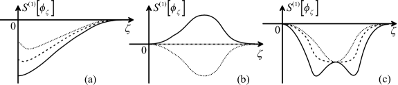
FIG. 3.: Three typical cases of the behavior of the Euclidean action as a function of $\zeta$ when a model parameter is varied.

As an example of $S^{(1)}$, let us consider the one given by

$$S^{(1)}=\epsilon\int d\eta\,a_{b}^{4}\,V_{1},\quad V_{1}=H^{4}\sum_{n=0}^{4}\alpha_{n}\,\tilde{\phi}^{n},$$ (63)

where $\tilde{\phi}:=2(\phi/\phi_{*})-1$. In this case, $S^{(1)}[\phi_{\zeta}]$ can be calculated analytically as

$$S^{(1)}[\phi_{\zeta}]=\epsilon\left[{4\over 3}(\alpha_{0}+\alpha_{4})+{2(\alpha_{1}+\alpha_{3})\over\sinh^{3}\zeta}\left(\cosh\zeta\sinh\zeta-\zeta\right)+{4\alpha_{2}\over\sinh\zeta}\left(\zeta\coth\zeta-1\right)\right].$$ (64)

If we choose a one-parameter family of models, say, like $2(\alpha_{1}+\alpha_{3})=-2+\alpha$ and $4\alpha_{2}=3$, where $\alpha$ is the variable parameter, the situation as shown in Fig. 3(a) is realized. On the other hand, if we choose $2(\alpha_{1}+\alpha_{3})=-\alpha$ and $4\alpha_{2}=2\alpha$, the situation as shown in Fig. 3(b) is realized. Within this limited class of perturbations, the situation as shown in Fig. 3(c) is not realized.

V conclusion

We have investigated the negative mode problem associated with false vacuum decay with gravity. We have shown that the existence of a negative mode around a non-trivial Euclidean solution, called the Coleman-De Luccia bounce solution, is equivalent to that of a supercritical supercurvature mode in the perturbation spectrum of the quantum fluctuations in the open universe that appears inside the bubble. Supercritical supercurvature modes are those for which the mode functions diverge exponentially for large spatial radius in the open universe. Then we have proposed a conjecture that there exists no supercritical supercurvature mode. If this is true, there will be no negative mode around the Coleman-De Luccia bounce solution that dominates the process of false vacuum decay.

To investigate the validity of our conjecture, we have first provided a potential model that admits a continuous series of Coleman-De Luccia type bounce solutions under the weak gravitational backreaction approximation. This series contains a Hawking-Moss type solution as a limiting case and each of these bounce solutions has a zero mode as the lowest eigenvalue. Then for a class of potentials that can be realized by small modifications of this potential model, we have analyzed the behavior of the Euclidean action around a bounce solution. We have shown that its Euclidean action is not the smallest among non-trivial solutions if there exists a negative mode.

We have considered three typical cases of the behavior of the action when a model parameter is varied. In all of these cases, we have found that, when there appears a bounce solution with a negative mode, it does not give the smallest action but there exists another bounce solution, either Coleman-De Luccia type or Hawking-Moss type, with a lower action that has no negative mode. This evidence strongly supports the conjecture that there is no negative mode for the Coleman-De Luccia bounce solution that dominates the tunneling process.

Acknowledgments

We thank J. Garriga for helpful discussions. This work was supported in part by the Monbusho Grant-in-Aid for Scientific Research No. 09640355 and by the Saneyoshi foundation.

REFERENCES

- [1] S. Coleman, Phys. Rev. D15, (1977), 2929; in The Whys of Subnuclear Physics, Proceedings of the International School, Erice, Italy, ed. A. Zichichi, Subnuclear Series Vol.15 (Plenum, New York. 1979), p.805.
- [2] C. G. Callan, Jr. and S. Coleman, Phys. Rev .D16(1977), 1762.
- [3] S. Coleman and F. De Luccia, Phys. Rev. D21 (1980), 3305.
- [4] T. Tanaka and M. Sasaki, Prog. Theor. Phys. 88 (1992), 503.
- [5] G. W. Gibbons, S.W. Hawking and M.J. Perry, Nucl. Phys. B138 (1978), 141.
- [6] M. Sasaki, T. Tanaka and K. Yamamoto, Phys. Rev. D51 (1995), 2979.
- [7] D.H. Lyth and A. Woszczyna, Phys. Rev. D52 (1995), 3338.
- [8] J. Garriga, X. Montes, M. Sasaki and T. Tanaka, in preparation.
- [9] G. Lavrelashvili, gr-qc/9804056.
- [10] S.W. Hawking and N. Turok, Phys. Lett. B425 (1998), 25.
- [11] J. Garriga, X. Montes, M. Sasaki and T. Tanaka, Nucl. Phys. B513 (1998), 343.
- [12] S. Coleman, Nucl. Phys. B298 (1988), 178.
- [13] J. L. Gervais and B. Sakita, Phys. Rev. D15 (1977), 3507.
- [14] S. Fubini, Nuovo Cimento 34A (1976), 521.
- [15] S.W. Hawking and I.G. Moss, Phys. Lett. 110B (1982), 35.