Phase diagram of the mean field model of simplicial gravity

Abstract

We discuss the phase diagram of the balls in boxes model, with a varying number of boxes. The model can be regarded as a mean-field model of simplicial gravity. We analyse in detail the case of weights of the form $p(q)=q^{-\beta}$, which correspond to the measure term introduced in the simplicial quantum gravity simulations. The system has two phases : elongated (fluid) and crumpled. For $\beta\in(2,\infty)$ the transition between these two phases is first order, while for $\beta\in(1,2]$ it is continuous. The transition becomes softer when $\beta$ approaches unity and eventually disappears at $\beta=1$. We then generalise the discussion to an arbitrary set of weights. Finally, we show that if one introduces an additional kinematic bound on the average density of balls per box then a new condensed phase appears in the phase diagram. It bears some similarity to the crinkled phase of simplicial gravity discussed recently in models of gravity interacting with matter fields.

The mean field description of simplicial gravity introduced in [1, 2, 3] was analysed in the series of papers [4, 5, 6]. As discussed there, the mean field approximation explains many facts observed in numerical experiments of simplicial gravity, such as the appearance of singular vertices and the mother universe, and the discontinuity of the phase transition. Recent work [7, 8] shows that adding vector matter fields to simplicial gravity effectively amounts to renormalising the $\alpha$ parameter in the measure term $q^{\alpha}$ where $q$ is the vertex order. The resulting phase diagram resembles the phase diagram of the mean–field model which we discuss in detail in this letter.

The model is given by the partition function [3] :

$$Z(N,\kappa,\beta) = \sum_{M=1}^{M_{max}}e^{\kappa M}\sum_{q_{1},\ldots,q_{M}}p(q_{1})\cdots p(q_{M})\delta{q_{1}+\cdots+q_{M},N}$$ (1)

$$= \sum_{M=1}^{M_{max}}e^{\kappa M}z(N,M,\beta)$$ (2)

It describes an ensemble of $N$ balls distributed in a varying number of boxes, $M$. The system has at least one box and at most $M_{max}$ boxes. The partitions of balls are weighted by the product of one-box weights $p(q)$, where $q$ is the number of balls in the box. Here we consider one parameter family of weights :

$$p(q)=q^{-\beta}\quad\mbox{for}\quad q=1,2,\dots\,.$$ (3)

Note that for these weights the minimal number of balls in a box is $q_{min}=1$. If there are no further constraints this implies that the maximal number of boxes is equal to the number of balls $M_{max}=N$.

For large $N$ the partition functions $z(\ldots)$ and $Z(\ldots)$ are expected to behave as :

$$z(N,M,\beta)\sim N^{y}e^{Nf(r,\beta)}\quad\mbox{with}\quad r=\frac{M}{N}\,,$$ (4)

and

$$Z(N,\kappa,\beta)\sim N^{Y}e^{N\phi(\kappa,\beta)}$$ (5)

where $f(r,\beta)$ and $\phi(\kappa,\beta)$ are appropriate thermodynamic potential densities depending on the intensive quantities characteristic for the $(r,\beta)$ and $(\kappa,\beta)$ ensembles. The power law corrections for the partition functions with the exponents $y$, $Y$ disappear in the thermodynamic limit. In our case they are the leading corrections. In general, however, there might be stronger corrections, for example of the type $\exp cN^{\alpha}$, with $\alpha<1$.

Substituting the summation in (2) by an integration over a continuous variable, we can relate the partition functions by the transform :

$$N^{Y}e^{N\phi(\kappa,\beta)}=N^{y+1}\,\int\limits_{0}^{1}\!\!\mbox{d}re^{N(f(r,\beta)+r\kappa)}\,,$$ (6)

The additional factor $N$ on the right hand side of (6) comes from the integration measure $Ndr$. In the thermodynamic limit, this gives :

$$\phi(\kappa,\beta)=f(r_{*},\beta)+r_{*}\kappa\,.$$ (7)

where $r_{*}$ is maximum of the integrand in (6). The value of $r_{*}$ is given by the equation :

$$-\kappa=\partial_{r}f(r_{*},\beta)$$ (8)

if the maximum of the integrand lies inside the interval $(0,1)$ and is equal $r_{*}=0$ or $r_{*}=1$ otherwise. Additionally we see that in the case when the maximum lies inside the interval $(0,1)$ the integration over $r$ around the saddle point introduces the additional factor $N^{-1/2}$. This leads to the following relation between the exponents $y$ and $Y$ :

$$Y=y+\frac{1}{2}\,.$$ (9)

Otherwise, the maximum lies at either end of the interval and the integration over $r$ introduces a factor $N^{-1}$, thus

$$Y=y\,.$$ (10)

We shall return to the exponents $Y,y$ later, concentrating now on the thermodynamic limit.

In the $(\kappa,\beta)$ ensemble one defines the average $\langle r\rangle$ :

$$\langle r\rangle=\frac{\langle M\rangle}{N}=\frac{1}{N}\frac{\partial_{\kappa}Z(N,\kappa,\beta)}{Z(N,\kappa,\beta)}\,.$$ (11)

As we will see this quantity plays the role of the order parameter. In the thermodynamic limit the equation (11) reads :

$$\langle r\rangle=\partial_{\kappa}\phi(\kappa,\beta)=r_{*}\,.$$ (12)

The second equality in the last formula can be treated as an inverse transform to (8). It results from the fact that the integrand of (6), which corresponds to the distribution of $r$, is sharply peaked around $r_{*}$ when $N\rightarrow\infty$ and the position of the peak also becomes the average of the distribution.

The task of determining $r_{*}$ relies on finding the maximum of the function $f(r,\beta)+\kappa r$. The function $f(r,\beta)$ can be found by the saddle point method [2] :

$$f(r,\beta)=\mu_{*}(r)+rK(\mu_{*}(r),\beta)$$ (13)

where $\mu_{*}(r)$ is a value which maximises the right hand side of the above expression for the given $r$. The function $K(\mu,\beta)$ is defined as :

$$K(\mu,\beta)=\log\sum_{q=1}^{\infty}p(q)e^{-\mu q}\,.$$ (14)

The properties of the function $K(\mu,\beta)$ are central to the further considerations as they fully determine the behaviour of the model. For the particular choice of weights (3) :

$$K(\mu,\beta)=\log\sum_{q=1}^{\infty}q^{-\beta}e^{-\mu q}=\log g_{\beta}(\mu)$$ (15)

where $g_{\beta}(\mu)$ is a function familiar from Bose-Einstein condensation, which has an integral representation :

$$g_{\beta}(\mu)=\frac{1}{\Gamma(\beta)}\int_{0}^{\infty}\frac{t^{\beta-1}dt}{e^{\mu+t}-1}\,.$$ (16)

The function $g_{\beta}(\mu)$ is defined on the interval $[0,\infty)$, so $\mu_{*}$ is either a solution of the saddle point equation :

$$\frac{1}{r}=-{\partial_{\mu}K(\mu_{*},\beta)}=\frac{g_{\beta-1}(\mu_{*})}{g_{\beta}(\mu_{*})}$$ (17)

for $r>r_{cr}$ or else $\mu_{*}=0$. The critical value of $r$ is

$$r_{cr}=\left\{\begin{array}[]{lr}0&\beta\leq 2\\ \frac{\zeta(\beta)}{\zeta(\beta-1)}&\beta>2\end{array}\right.\,,$$ (20)

where $\zeta(\beta)$ is the Riemann Zeta function which arises when one inserts $\mu_{*}=0$ into $K(\mu,\beta)$ in (15). For $r<r_{cr}$ the function $\mu+rK(\mu,\beta)$ has no maximum in the range $(0,\infty)$ and $\mu_{*}=0$.

We thus see that the function $f(r,\beta)$ as a function of $r$ changes regime at $r=r_{cr}$. For $r<r_{cr}$ ie $\mu_{*}=0$ the equation (13) reduces to the linear dependence :

$$f(r,\beta)=-\kappa_{cr}(\beta)\,r$$ (21)

where

$$-\kappa_{cr}=\log\zeta(\beta)\,.$$ (22)

We have added the minus sign in the definition of $\kappa_{cr}$ for convenience to adjust to the sign in the saddle point formula (8).

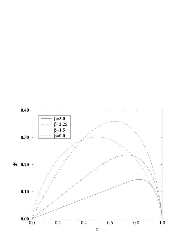
Figure 1: The $f(r,\beta)$ for various values of $\beta$. The curves for $\beta>2$ possess a linear part at $r=0$. The main difference between the curves for $\beta=0$ and $\beta=1.5$ is the former has an infinite derivative $\partial_{r}f$ at $r=0$, whereas the latter has a finite derivative. For all the curves the derivative at $r=1$ is infinite. See figure 2.

The function $f(r,\beta)$ as a function of $r$ has different qualitative behaviour depending on $\beta$. For $\beta>2$ the function has a linear piece for $r<r_{cr}$. This piece becomes shorter when $\beta$ approaches $2$ and finally disappears. For $1<\beta<2$ the function has no linear piece, but it does have a finite derivative at $r=0$. This distinguishes this range from $\beta<1$ where the derivative $\partial_{r}f$ at $r=0$ is infinite. Representative shapes of the function $f$ for $\beta$ from the three ranges are shown in figure 1. This figure is supplemented by figure 2 where the derivative is plotted to expose its behaviour at $r=0$. With this picture in mind one can see the main feature of the solution $r_{*}$ of the saddle point equation (8). Namely, for $\beta<1$, for each $\kappa$ it has always a solution in the range $(0,1)$. For $1<\beta<2$, $r_{*}$ lies in the range $(0,1)$ so long as $\kappa>\kappa_{cr}$, whereas $r_{*}=0$ for $\kappa\leq\kappa_{cr}$. Finally, for $\beta>2$, the solution lies in the range $(r_{cr},1)$ for $\kappa>\kappa_{cr}$ and then jumps to $r_{*}=0$ for $\kappa\leq\kappa_{cr}$. This is illustrated in figure 3.

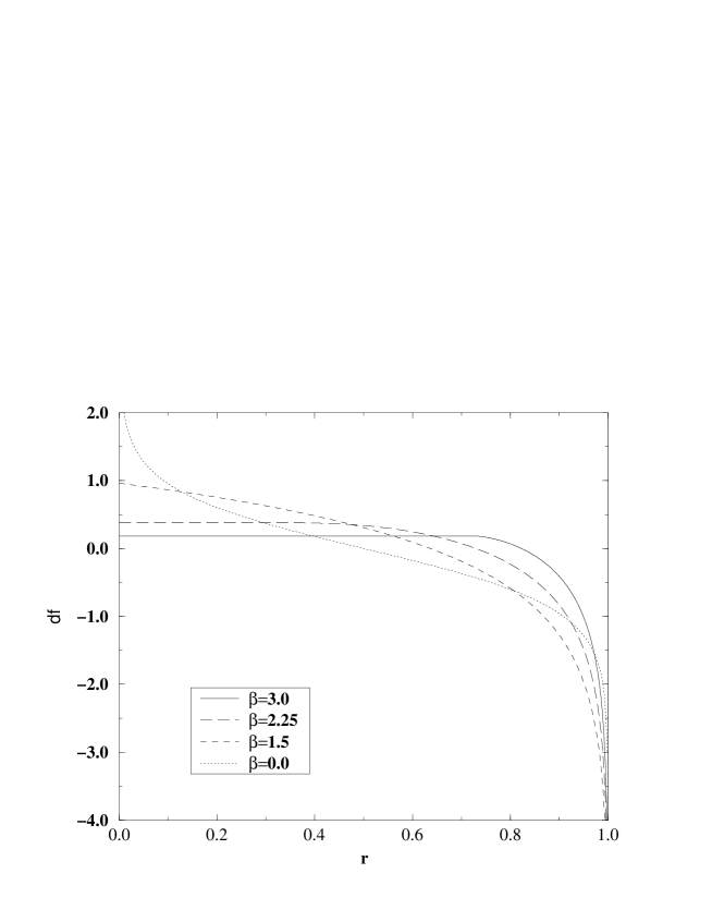
Figure 2: The derivative $\partial_{r}f(r,\beta)$ of the curves from the figure 1. All go to infinity at $r=1$. Depending on the value of $\beta$ they drastically change behaviour at $r=0$ : for $\beta=0$ they go to infinity, for all other are finite. For $\beta=2.25$ and $\beta=3.0$ they are constant in some range of $r$.

Figure 3: The value of $r_{*}(\kappa)$ for various values of $\beta$. The portions of plots lying on the $x$ axis ($r_{*}=0$) are not plotted.

The discontinuity at $\kappa=\kappa_{cr}$ (22) has the height $r_{cr}$ given by (20). The average $\langle r\rangle=r_{*}$ is an order parameter for the model. A simple consequence of equation (20) is that the transition becomes continuous when $\beta=2$ since $r_{cr}=0$. In fact, the transition stays continuous as long as $\beta$ is in the range $(1,2]$. In this range the $r_{cr}=0$ and $\kappa_{cr}$ is finite and given by (22). As $\beta$ approaches unity, $\kappa_{cr}\to-\infty$ and the transition disappears. This process is illustrated in figure 3. For $\beta<1$ the values of the derivative $\partial_{r}f(r,\beta)$ span the interval $(-\infty,\infty)$ and the saddle point equation (8) always has a nonzero solution $r_{*}$ for the whole range of $\kappa$. The model therefore has only one phase and no phase transition. To illustrate this, consider the solution when $\beta=0$ :

$$r_{*}=\frac{1}{1+e^{-\kappa}}\,,$$ (23)

which is a smooth function spanning the range $(0,1)$ without any singularity.

The phase diagram in the $(\kappa,\beta)$ plane is drawn in figure 4.

Figure 4: The phase diagram. The continuous line denotes a first-order phase transition. The dashed line denotes a continous transition. The dotted line shows the transition line that appears after addition of the artificial cut-off.

The solid line is a discontinuous phase transition with a nonzero gap $r_{cr}$ (20) while the dashed line is a continuous transition.

Coming back to the range $(1,2)$ of $\beta$ one can determine the singularity type of the thermodynamical functional $\phi(\kappa,\beta)$ at the transition ie when $\kappa\rightarrow\kappa_{cr}$. For small $\mu$ :

$$g_{\beta}(\mu)=\Gamma(1-\beta)\mu^{\beta-1}+\sum_{k=0}^{\infty}\zeta(\beta-k)\frac{-\mu^{k}}{k!}\,.$$ (24)

Inserting this into the equation (17) one obtains for small $\mu$ :

$$r\sim\mu^{2-\beta}+\dots\quad,$$ (25)

or, after inverting it for $\mu$ :

$$\mu_{*}\sim r^{1/(2-\beta)}\,.$$ (26)

In this range of $\beta$ $r_{cr}=0$ and so $\mu_{*}$ is given by the equation :

$$\kappa=-\log g_{\beta}(\mu_{*})$$ (27)

For small $\mu_{*}$ we can write :

$$\kappa-\kappa_{cr}=-\log g_{\beta}(\mu_{*})+\log\zeta(\beta)\sim\mu^{\beta-1}\sim r^{(\beta-1)/(2-\beta)}\,.$$ (28)

Inverting this with respect to $r$ we eventually get :

$$\langle r\rangle=r_{*}\sim(\kappa-\kappa_{cr})^{x},\makebox[56.9055pt]{where}x=\frac{2-\beta}{\beta-1}\quad.$$ (29)

The exponent $x$ varies between $\infty$ and $0$ as $\beta$ grows from one to two. In the limiting case $\beta\rightarrow 1$, the exponent $x\rightarrow\infty$ which means that the singularity becomes arbitrarily soft, which perfectly matches the fact that for $\beta<1$ there is no singularity. At the other end of the interval, when $\beta\rightarrow 2$, the exponent $x\rightarrow 0$, which means that $\langle r\rangle$ becomes an arbitrarily steep function at $\kappa_{cr}$ which again agrees with the fact that for $\beta>2$ the function is discontinuous at $\kappa_{cr}$.

What we have discussed so far is an extension and refinement of the analysis of the model presented in [3]. A few comments are in order. The analysis can be generalised for an arbitrary set of weights. In general, the transition takes place when the argument $e^{-\mu}$ of the series (14) approaches the radius of convergence of the series. Denote the radius by $e^{\Delta}$. In our example the radius was $1$ ie $\Delta=0$, but in general $\Delta$ may be any finite number. The condition for the existence of the transition is that the generating function $K$ (14) is finite at the radius of convergence of the series :

$$K(\Delta,\beta)<\infty\,.$$ (30)

The family of weights may be parametrised by many parameters. In the last formula, the parameters are represented by a single symbol $\beta$. The equation :

$$-\kappa_{cr}=K(\Delta,\beta)\,,$$ (31)

is the equation of the critical line between the phases of the $(\kappa,\beta)$ ensemble. Moreover, as one can see by repeating the arguments previously used for the particular weights (3), the condition for the transition to be discontinuous is :

$$\partial_{\mu}K(\Delta,\beta)<\infty$$ (32)

since the inverse of the derivative $\partial_{\mu}K$ corresponds to the latent heat. The transition is continuous for $\beta$’s for which the latent heat vanishes and condition (30) is fulfilled.

The position of the critical line on the phase diagram can be easily changed by a slight modification of weights. For example, a simple multiplication by a constant $C$ : $p(q)\rightarrow Cp(q)$ corresponds to a horizontal shift of the critical line in the phase diagram (Fig. 4). In general a slight modification of weights can also change the $\beta$ position of critical line and thus the critical exponent (29). In this respect this model is “non-universal” (see also [9]).

So far we have discussed the behaviour of the model in the thermodynamic limit. We now determine the exponents $y$ (4) and $Y$ (5). It is convenient to define the grand canonical partition function :

$${\cal Z}(\mu,\kappa,\beta)=\sum_{N=1}^{\infty}e^{-N\mu}Z(N,\kappa,\beta)\sim(\mu-\mu_{0})^{-1-Y}\,,$$ (33)

whose singularity type depends on the exponent $Y$. The critical value of the chemical potential is $\mu_{0}=\phi(\kappa,\beta)$ is zero in the crumpled and nonzero in the fluid phase. The value of the exponent $Y$ depends also on the position $(\kappa,\beta)$ in the phase diagram. From (2) one obtains the following expression :

$${\cal Z}(\mu,\kappa,\beta)=\frac{e^{\kappa}g_{\beta}(\mu)}{1-e^{\kappa}g_{\beta}(\mu)}\,$$ (34)

from which one can extract the singularity. In the fluid phase, the singularity comes from the residual denominator and it is :

$${\cal Z}(\mu,\kappa,\beta)\sim(\mu-\mu_{0})^{-1}\,,$$ (35)

from which one concludes that $Y=0$.

For $(\kappa,\beta)$ in the crumpled phase, the singularity comes from the numerator of the fraction (34) which itself has a power like singularity when $\mu$ approaches $\mu_{0}=0$. Thus

$${\cal Z}(\mu,\kappa,\beta)\sim\mu^{\beta-1}$$ (36)

and hence $Y=-\beta$. In other words, the partition function inherits the singularity from the weights or more precisely from the generating function $K(\mu,\beta)$. This effect comes from the dominance of the singular box contribution over the negligible entropy. In general the singularity need not be power like. For example the weights : $p(q)=\exp(-aq+bq^{1/2})$, where $a$ and $b$ are positive constants, would lead to an essential singularity. In this case $N^{Y}$ would not be the dominant correction to the partition function.

Let us now determine the singularity type on the critical line. The singularity comes from the denominator in the expression (34). It changes at $\beta=2$. For $\beta>2$ the expansion of the denominator in small $\mu$ begins with the linear term. Because the numerator approaches a non-vanishing constant for $\mu\rightarrow 0$, we have :

$${\cal Z}(\mu,\kappa,\beta)\sim\mu^{-1}\,,$$ (37)

and hence $Y=0$ as in the fluid phase. For $1<\beta<2$ the expansion of the denominator begins with the singular term $\mu^{\beta-1}$ (16), thus

$${\cal Z}(\mu,\kappa,\beta)\sim\mu^{1-\beta}\,,$$ (38)

and $Y=-2+\beta$.

So far we have tacitly set $q_{min}=1$, which meant that each box contained at least one ball. As a result, the system with $N$ balls could have $M$ boxes at most. Hence the maximal value of $r$ is $1$. If one instead chooses $q_{min}$ to be larger than one then the maximal $r$ is :

$$r_{max}=1/q_{min}\,.$$ (39)

In this case, the analysis of the model proceeds exactly as before, except that in place of $1$ for the upper limit one sets $r_{max}=1/q_{min}$. In particular, the range of integration in equation (6) is now $(0,r_{max})$ and the derivative $\partial_{r}f$ is infinite at $r_{max}$. The average $\langle r\rangle$ approaches asymptotically $r_{max}$ when $\kappa\rightarrow-\infty$. So the only essential difference to the previous analysis is the range of $r$. In particular, the phase structure of the model is unchanged. We shall call $r_{max}$ the natural limit for $r$.

The phase structure of the model can be made more complex by introducing a slight modification. Let us impose a kinematic upper limit on $r$. We shall call this the artificial limit and denote it by $r_{art}$. The artificial limit obviously has to lie below the natural one, $r_{art}<r_{max}$. Now the partition function becomes :

$$N^{Y}e^{N\phi(\kappa,\beta)}=N^{y+1}\,\int\limits_{0}^{r_{art}}\mbox{d}re^{N(f(r,\beta)+r\kappa)}\,.$$ (40)

The main difference between the natural and the artificial limit is that the derivative $\partial_{r}f$ is infinite at the former and finite at the latter. In the case of a model with the natural limit, this limit is never reached by the average $\langle r\rangle$, or at worst reached only asymptotically for $\kappa\rightarrow-\infty$, whereas the artificial limit can be reached for finite $\kappa$ when the term $r\kappa$ dominates over $f(r,\beta)$ in the integrand (40). If we fix $\beta$ and change $\kappa$ from large positive values towards large negative, the system is first in the condensed phase $\langle r\rangle=0$, then at the critical value $\langle r\rangle$ jumps to $r_{cr}$ and later smoothly rises until it reaches $r_{art}$ where it sticks (see figure 5). Such a situation is very similar to the previous standard one.

There exists, however, the possibility of quite different behaviour. For $\beta>\beta_{*}$ where $\beta_{*}$ is defined by the equation :

$$r_{art}=\frac{\zeta(\beta_{*})}{\zeta(\beta_{*}-1)}$$ (41)

the value of $r_{cr}$ is larger than $r_{art}$. In this case, at the transition from the condensed phase $\langle r\rangle$ jumps from zero directly to $r_{art}$. It cannot jump to $r_{cr}$ because this lies above $r_{art}$ and is beyond the allowed kinematic range (figure 5).

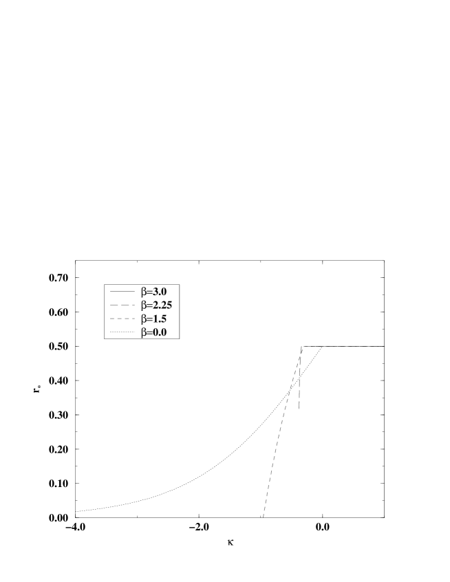
Figure 5: The dependence $r_{*}$ on $\kappa$ for various values of $\beta$ in presence of the artificial cut-off

This gives a new phase which is neither crumpled nor fluid. It has $\langle r\rangle>0$ but on the other hand there is a singular box in the system. We call this phase condensed, as it is analogous to the condensed phase of the canonical $Z(M,N,\beta)$ ensemble. We have marked the critical line separating the condensed phase from fluid one by the dotted line on the phase diagram in the figure 4.

Define the quantity :

$$\langle s\rangle=\frac{\langle q_{sing}\rangle}{N}\,,$$ (42)

which is the fraction of all balls which are in the singular box. The quantities $\langle r\rangle$ and $\langle s\rangle$ play the role of the order parameters. We have :

$$\begin{array}[]{lll}\mbox{crumpled~{}:}&\langle r\rangle=0\,,&\langle s\rangle=1\,,\\ \mbox{fluid~{}:}&\langle r\rangle>0\,,&\langle s\rangle=0\,,\\ \mbox{condensed~{}:}&\langle r\rangle>0\,,&\langle s\rangle>0\,.\\ \end{array}$$ (46)

The phase diagram is very similar to the one of simplicial gravity with the matter fields or the measure term [7, 8]. If one naively applies the mean field model to 4d simplicial gravity one would get the following constraint for the orders of vertices :

$$q_{1}+q_{2}+\dots+q_{N_{0}}=5N_{4}$$ (47)

where $N_{0}$ is the total number of vertices, $q_{i}$ the order of vertex $i$, and $N_{4}$ is the number of 4simplices. We thus have the correspondence $N_{0}\leftrightarrow M$, $\kappa_{0}\leftrightarrow-\kappa$ and $N_{4}\leftrightarrow N$. The minimal order of a vertex is $q_{min}=5$, so the natural limit $r_{max}=1/5$. This means that :

$$\frac{\langle N_{0}\rangle}{N_{4}}=1$$ (48)

is the natural upper limit for $\langle N_{0}\rangle/N_{4}$ from the point of view of the mean field model. As we know this limit is never reached since the simplicial structure imposes the limit $\langle N_{0}\rangle=1/4$ which in the language of the mean field model corresponds to the artificial upper limit[11]. The full 4d theory thus provides the structure which we have assumed in the discussion of the mean–field model. Of course, the cut off at $1/4$ is not as sharp as we have assumed. One expects a smooth cut off, which means that the entropy of configurations for $\langle N_{0}\rangle/N_{4}$ approaching $1/4$ gradually decreases in comparison with the mean field model, so that the upper limit $\langle N_{0}\rangle/N_{4}=1/4$ is not reached at finite $\kappa_{0}$ but rather asymptotically approached for large $\kappa_{0}$.

The source of the limit $\langle N_{0}\rangle/N_{4}=1/4$ in simplicial gravity is purely geometrical and results from the fact that $q_{i}$ is the number of 4-simplices. A consequence of this is that if we add a point with $q_{i}=5$, for example by a barycentric subdivision, we increase the numbers $q_{j}$ of neighbouring vertices[11]. In other words, $q_{i}$’s are not independent and in particular one cannot make all of them equal to $5$ as the natural limit would require.

The exponent $Y$ requires some comment. In the theory of random geometries one defines the string susceptibility exponent $\gamma$, which is the counterpart of $Y$. The exponents $Y$ is shifted by a constant with respect to the standard definition of $\gamma$ : $Y=\gamma-3$. If one followed these definitions in the fluid phase one would obtain $\gamma=3$ in the $(\kappa,\beta)$ ensemble since, as we have seen, $Y=0$. However, the mean field model neglects all the subtle effects and combinatorial factors coming from topological constraints imposed by the local geometry so one should treat this value with some caution.

Similarly, the crumpled phase of the ball in boxes model has $Y=-\beta$, but the following argument suggests that the corresponding value of $\gamma$ is not that which is naively expected. The balls in boxes model in the particular case of the $r=1/2$ ensemble can be mapped onto the branched polymer model with the topology of sphere [2, 9]. One can recognise the fluid phase of the balls in boxes model as the generic phase of the branched polymer model. For the former $y=-1/2$, whereas for the latter $\gamma=1/2$, from which one can conjecture $y=\gamma-1$. Switching back to the varying number of boxes ensemble we have $Y=y$ in the crumpled phase from equation (10), and $\gamma=1-\beta$.

To calculate $\gamma$ and hence $Y,y$ in the condensed phase we will use a heuristic argument. We know that $Y=y$ since the phase is again on the kinematic border (10), as for the crumpled phase, but $y$ is now the exponent of the fixed $r=r_{art}$ ensemble. As before, in the particular case $r=1/2$ we can take the value of $\gamma=2-\beta$ from the branched polymer model ([9]). If we assume that this relation holds independently of $r$, and that $y=\gamma-1$ as conjectured above for the crumpled phase, we obtain $Y=y=1-\beta$ which differs by one from the crumpled phase value.

We think that the main feature of the mean–field solution is that the exponent $\gamma$ properly reflects an universal behaviour, ie it is independent on the location in the phase diagram as long as the system is in the fluid phase. This is more important in the context of simplicial gravity than the particular predictions for the exponent $\gamma$ calculated for our choice of power law weights. Mean field theories will, in any case, generically predict critical exponents incorrectly.

In summary, we have seen that the mean field model of simplicial quantum gravity can account for many of the features seen in simulations of the full model. With the correct choice of ensemble (a varying number of boxes) we reproduce the first order nature of the transition for for $\beta\in(2,\infty)$, while for $\beta\in(1,2]$ it is continuous, disappearing altogether at $\beta=1$. We have also remarked that taking further account of the local geometrical constraints in the model can be implemented as a lowered limit on the region of integration in the saddle point equation, which we have denoted as the artificial upper limit. With the artificial limit in place we found the modified phase diagram of figure 4, which possesses a new condensed phase. This is similar to the crinkled phase of full simplicial gravity with matter fields or the (apparently equivalent) measure term [7, 8].

References

- [1] P. Bialas, Z. Burda, B. Petersson, J. Tabaczek Nucl. Phys. B495 (1997) 463.
- [2] P. Bialas, Z. Burda, D. Johnston Nucl. Phys. B493 (1997) 505.
- [3] P. Bialas, Z. Burda, Phys. Lett. B416 (1998) 281.
- [4] S. Catterall, J. Kogut, R. Renken Phys. Lett. B416 (1998) 274.
- [5] S. Catterall , J. Kogut, R. Renken Phase structure of dynamical triangulation models in three-dimensions. hep-lat/9712011 (To be published in NP)
- [6] Z. Burda, Acta Phys. Pol B29 (1998) 573.
- [7] S. Bilke, Z. Burda, A. Krzywicki, B. Petersson, J. Tabaczek, G. Thorleifsson, Phys. Lett. B418 (1998) 266.
- [8] S. Bilke, Z. Burda, A. Krzywicki, B. Petersson, J. Tabaczek, G. Thorleifsson, 4-d simplicial quantum gravity: matter fields and the corresponding effective action, hep-lat/9804011 to be published in Phys. Lett. B
- [9] P. Bialas, Z. Burda Phys. Lett. B384 (1996) 75.
- [10] J. Ambjorn, J. Jurkiewicz, Nucl. Phys. B451 (1995) 643.
- [11] D. Walkup, Acta Math. 125 75.