Gravitation Theory with Propagating Torsion

Abstract

We present a review of some recent models of gravitation theory with propagating torsion based on the use of a torsion-dilaton field and propose one more model of this type which promises to be more realistic. A proper universal self-consistent minimal action principle yields the properties of this model and predicts the interactions of torsion-dilaton field with the real matter. The new model may be compatible with the string models with dilaton field and gives a novel interpretation of the dilaton as a part of the space-time torsion. A relation with some recent models of dilatonic gravity is also possible.

1 Introduction

The affine geometry with torsion was invented by E. Cartan in 1922 [1]. He suggested, too the idea to enlarge the framework of general relativity using this geometry which is more general then Riemannian one. Today the affine geometry has got many applications in different physical theories. Here is a list of part of them:

1. Einstein-Cartan (EC) theories (See for example [2] – [7] and the references there in);

2. Gauge theories of gravity – Einstein-Cartan-Sciama-Kible (ECSK) theories (See for example [2] – [7] and the references there in);

3. Affine-metric theories of gravity (See for example the review article [7] and the huge amount of references there in);

4. Theory of supergravity (see for example [5], [8] and the references there in);

5. All kinds of modern superstring theories (See for example [9], [10], the recent review article [11] and the references therein).

6. Theory of ”strong gravity” (see for example [5], and the references there in);

7. Theory of the gravitational singularities [12], [13];

8. Theory of the plastic deformations in solid states (see for example [14] – [16], and the references there in);

9. Theory of space-time defects (See for example [17] – [21], and the references there in);

10. Theory of the Kustaanheimo-Stiefel transformation in celestial mechanics [22] and the corresponding extension in quantum mechanics, especially, the Duru-Kleinert transformation in calculation of the Feynman path integral for Colomb potential (see for example [16] and the references there in);

11. Recently proposed new formulation of the very general relativity in terms of teleparallel spaces [23] – [25];

12. Low energy limit of string theory (See for example [9], [10], [26] – [28]); and so on. There exist a huge amount of papers on these subjects and one may find the corresponding references in the literature, cited above. Unfortunately, no well established physical results which manifest the usefulness of the torsion in the fundamental physics were found up to now. Therefore a lot of people do not believe in torsion. Nevertheless at present a not very big scientific community still continue to propose new models of gravity with torsion and to hope to realize after all the fundamental Cartan idea as a part of modern development of physical theory.

The purpose of this article is to represent the recent investigations of the model of gravity with propagating torsion proposed by A. Saa in [29] – [33] which ware performed by the author and his collaborators, as far as some new models [34] – [37] which are aimed to overcome the theoretical and experimental inconsistencies of Saa’s model. Some of these new models are based on the previous researches on the action principle in spaces with torsion [38] – [43]. Finally we formulate one more new model of gravitation with propagating torsion-dilaton which promises to be more realistic.

2 The Self Consistent Minimal Coupling Principle Problem in Spaces with Torsion

We shell start remaining some well known basic notions and definition from differential geometry to adjust the terminology and notations we will use further. We denote as ${\cal M}^{(1,3)}\{g_{\alpha\beta}(x),\Gamma^{\gamma}_{\alpha\beta}(x)\}$   the affine connected space with connection coefficients $\Gamma^{\gamma}_{\alpha\beta}(x)$ and metric tensor $g_{\alpha\beta}$ with signature (+,-,-,-). This four-dimensional affine-metric space will be our model of the physical space-time in what follows. The connection and the metric in it further are supposed to be related in general only by the metricity condition: $\nabla_{\alpha}g_{\beta\gamma}\equiv 0$, $\nabla_{\alpha}$ being the covariant derivatives with respect to the affine connection with coefficients $\Gamma^{\gamma}_{\alpha\beta}$. This metricity condition yields the important relation $\Gamma^{\gamma}_{\alpha\beta}={\gamma\brace\alpha\beta}+{K_{\alpha\beta}}^{\gamma}$ where ${\gamma\brace\alpha\beta}={{\small\,\,\hbox{${\frac{1}{2}}$}}}g^{\gamma\mu}(\partial_{\alpha}g_{\mu\beta}+\partial_{\beta}g_{\mu\alpha}-\partial_{\mu}g_{\alpha\beta})$ are the Christoffel symbols, i.e. the coefficients of the Levi-Civita connection, ${K_{\alpha\beta}}^{\gamma}={S_{\alpha\beta}}^{\gamma}+{S^{\gamma}}_{\alpha\beta}+{S^{\gamma}}_{\beta\alpha}$ is the contorsion tensor, and ${S_{\alpha\beta}}^{\gamma}=\Gamma^{\gamma}_{[\alpha\beta]}$ is the torsion tensor (in coordinate basis). We shall need the torsion vector $S_{\alpha}={{\small\,\,\hbox{${\frac{2}{D-1}}$}}}{S_{\alpha\mu}}^{\mu}={\frac{2}{3}}{S_{\alpha\mu}}^{\mu}$ for dimension $D=1+3$ of the space-time . As we see, due to the metricity condition the torsion enters into the symmetric part of the connection coefficients, too: $\Gamma^{\gamma}_{\{\alpha\beta\}}={\gamma\brace\alpha\beta}+{S^{\gamma}}_{\alpha\beta}+{S^{\gamma}}_{\beta\alpha}$, nevertheless it was defined in a coordinate basis as an anti-symmetric part of these coefficients. As a result if the torsion tensor $S_{\alpha\beta\gamma}$ is not complete anti-symmetric in its three indexes the following specific problem (which we shell call ”the G-A problem”) appears in the affine-metric spaces:

Consider first the free motion of a relativistic particle with mass $m$ in a flat Minkowski space ${\cal E}^{(1,3)}\{\eta=(+1,-1,-1,-1),\Gamma=0\}$, $\eta$ being its metric. The action functional

$${\cal A}[x]=-mc\int\sqrt{\eta_{ij}dx^{i}dx^{j}}=-mc\int ds$$ (1)

under standard action principle

$$\delta{\cal A}[x]=0$$ (2)

leads to the dynamical equations:

$$mc^{2}{\frac{d^{2}x^{i}}{ds^{2}}}=0$$ (3)

solved by a straight lines with uniform velocity. These straightest lines are at the same time the shortest ones which connect the initial and the final position of the particle.

The standard minimal coupling principle (MCP) maps dynamical equations (3) onto the equations of motion:

$$mc^{2}\left({\frac{d^{2}x^{\gamma}}{ds^{2}}}+\Gamma_{\alpha\beta}^{\gamma}{\frac{dx^{\alpha}}{ds}}{\frac{dx^{\beta}}{ds}}\right)=mc^{2}{\frac{D}{ds}}{\frac{dx^{\gamma}}{ds}}=0,$$ (4)

which describe the straightest lines, i.e. the autoparallel lines (A-lines) in the space ${\cal M}^{(1,3)}\{g_{\alpha\beta}(x),\Gamma^{\gamma}_{\alpha\beta}(x)\}$,  ${\frac{D}{ds}}$ being the absolute derivative with respect to the affine connection, and the action (1) onto the action

$${\cal A}[x]=-mc\int\sqrt{g_{\mu\nu}(x))dx^{\mu}dx^{\nu}}=-mc\int ds.$$ (5)

But under standard action principle (2) this action functional yields the geodesic line (G-line) equations of motion which describe the lines with stationary length (sometimes called ”shortest lines”, nevertheless in general this may be not true) in the space ${\cal M}^{(1,3)}\{g_{\alpha\beta}(x),\Gamma^{\gamma}_{\alpha\beta}(x)\}$:

$$mc^{2}\left({\frac{d^{2}x^{\gamma}}{ds^{2}}}+{\gamma\brace\alpha\beta}{\frac{dx^{\alpha}}{ds}}{\frac{dx^{\beta}}{ds}}\right)=mc^{2}{\frac{D}{ds}}{\frac{dx^{\gamma}}{ds}}-2mc^{2}{S^{\gamma}}_{\alpha\beta}{\frac{dx^{\alpha}}{ds}}{\frac{dx^{\beta}}{ds}}=0.$$ (6)

Obviously the autoparallel equation (4) means a free motion of the test spinless particle in the space ${\cal M}^{(1,3)}\{g_{\alpha\beta}(x),\Gamma^{\gamma}_{\alpha\beta}(x)\}$ with zero absolute acceleration: $a^{\gamma}=c^{2}{\frac{D}{ds}}{\frac{dx^{\gamma}}{ds}}=0$. This is the most natural translation of the usual dynamics of test free particle and corresponds to the very physical notion of a ”free test particle”.

In contrast, the geodesic equations (6) imply in general the unnatural law of free motion:   $ma^{\gamma}={\cal F^{\gamma}}$. Hence, we actually have to introduce a specific ”torsion force” ${\cal F^{\gamma}}=2mc^{2}{S^{\gamma}}_{\alpha\beta}u^{\alpha}u^{\beta}$ ($u^{\alpha}={\frac{dx^{\alpha}}{ds}}$ being the particle’s four-velocity) to compensate the natural torsion dependence of the dynamics in the space ${\cal M}^{(1,3)}\{g_{\alpha\beta}(x),\Gamma^{\gamma}_{\alpha\beta}(x)\}$ and to allow the free test particle to follow the usual extreme of the classical action (5).

The same problem we observe in field dynamics of classical fields with different spin. In the simplest case of a massive spinless scalar field with mass $m$ the flat Minkowski equation of motion

$$\eta^{\mu\nu}\partial_{\mu}\partial_{\nu}\phi+m^{2}\phi=0$$ (7)

being derivable via standard action principle from the action integral

$${\cal A}[\phi(x)]=\int d^{4}x{{\small\,\,\hbox{${\frac{1}{2}}$}}}\!\left(\eta^{\mu\nu}\partial_{\mu}\phi\partial_{\nu}\phi-m^{2}\phi^{2}\right)$$ (8)

is mapped onto the autoparallel-type (A-type) equation

$$\Box\phi+m^{2}\phi=0$$ (9)

under the standard MCP which produces the action

$${\cal A}[\phi(x)]=\int d^{4}x\sqrt{|g(x)|}{{\small\,\,\hbox{${\frac{1}{2}}$}}}\!\left(g^{\mu\nu}\nabla_{\mu}\phi\nabla_{\nu}\phi-m^{2}\phi^{2}\right)$$ (10)

in the space ${\cal M}^{(1,3)}\{g_{\alpha\beta}(x),\Gamma^{\gamma}_{\alpha\beta}(x)\}$ (for scalar field $\nabla_{\mu}\phi\equiv\partial_{\mu}\phi$). Then the standard action principle yields the geodesic-type (G-type) equation of motion

$${\stackrel{{\scriptstyle{}^{\{\}}}}{{\Box}}}\phi+m^{2}\phi=\Box\phi+m^{2}\phi+3S^{\mu}\nabla_{\mu}\phi=0.$$ (11)

Here we use the laplasian $\Box=g^{\alpha\beta}\nabla_{\alpha}\nabla_{\beta}$ and Laplas-Beltrami operator ${\stackrel{{\scriptstyle{}^{\{\}}}}{{\Box}}}=g^{\alpha\beta}\stackrel{{\scriptstyle{\{\}}}}{{\nabla}}_{\alpha}\stackrel{{\scriptstyle{\{\}}}}{{\nabla}}_{\beta}={1\over\sqrt{|g|}}\partial_{\mu}\left(\sqrt{|g|}g^{\mu\nu}\partial_{\nu}\right)=\Box+3S^{\mu}\nabla_{\mu}$ in the space ${\cal M}^{(1,3)}\{g_{\alpha\beta}(x),\Gamma^{\gamma}_{\alpha\beta}(x)\}$, $\stackrel{{\scriptstyle{\{\}}}}{{\nabla}}_{\alpha}$ being the covariant derivative with respect to the Levi-Civita connection with coefficients ${\gamma\brace\alpha\beta}$.

The A-type equation (9) is essentially different from the G-type equation (11) if the torsion vector $S_{\alpha}$ does not vanish and this leads to the G-A problem in the case under consideration. If we consider the affine connection as a fundamental object which defines the very geometry of the space ${\cal M}^{(1,3)}\{g_{\alpha\beta}(x),\Gamma^{\gamma}_{\alpha\beta}(x)\}$ all equations of motion have to be written in terms of its absolute derivatives. Then the third term $3S^{\mu}\nabla_{\mu}\phi$ in the corresponding form of the equation (11) has to be considered as a density of an additional force ${\cal F}=-3S^{\mu}\nabla_{\mu}\phi$ caused by torsion. It has to be introduced to compensate the natural torsion dependence of the scalar field dynamics generated by the direct application of the MCP to the special relativistic equation of motion (7) of spinless field.

The above paradox in the description of the free motion of test particles and fields in affine connected spaces ${\cal M}^{(1,3)}\{g_{\alpha\beta}(x),\Gamma^{\gamma}_{\alpha\beta}(x)\}$ with nonzero torsion forces one to answer the following two basic questions:

1) What is more fundamental:

$\bullet$   the free motion as a motion without external forces of any nature, and hence, with zero absolute acceleration, according to Newton law of inertia; or

$\bullet$   the free motion as a motion governed by geodesic type of equations of motion in accordance with the standard action principle.

2) Do the self consistent minimal coupling principle (SCMCP) exist which will yield the same results when applied in action principle and directly in the equation of motion in flat Minkowski space.

Concerning the answer of the first question it is quite obvious that the Newton law of inertia has a more profound physical character.

In addition it is interesting to note that as early as in [45] a deep analysis of the origin of inertial forces, their relations with gravitation and the possibility of a geometric description of these two types of forces which look quite different at first glance brings Weyl to the conclusion that the inertia and the gravitation are to be determined by some affine connection. In Weyl’s analysis the free motion is just an autoparallel displacement of the particle velocity with respect to this affine connection. But after all without any physical motivation Weyl superimposes the ”usual” condition ${\Gamma_{\alpha\beta}}^{\gamma}={\Gamma_{\beta\alpha}}^{\gamma}$ and thus arrives to the standard Levi-Civita connection in general relativity.

The well known argument to chose the second alternative answering the first question is the fact, that the action principle follows from quantum mechanics as a fundamental principle for classical motion [46], [47]. But there is no guarantee that the quantum mechanics leads to the usual form of action principle in affine connected spaces with nonzero torsion. Moreover it is found that Feynman path integral leads to the Schrödinger equation of autoparallel type in such spaces [16], [48].

So, answering the first question it will be very hard to drop out from the physical theory one of the two well established principles which conflict in the presence of torsion. The best thing we can do will be to give a positive answer to the second question and this way to overcome the G-A problem. There exist two possibilities to do this: the first is to change the very variational principle, the second one is to change properly the action functional in spaces with torsion, i.e. to modify the minimal coupling principle in presence of torsion.

The autoparallel motion of test particle in affine connected spaces was proposed in [49] and derived from formally modified variational principle as early as in [38]. It was based on the following new postulate:

$$\biggl{(}\delta_{x}{\frac{d}{dt}}-{\frac{d}{dt}}\delta_{x}\biggr{)}x^{\alpha}=2{S_{\mu\nu}}^{\alpha}\dot{x}^{\mu}\delta x^{\nu}$$ (12)

for the commutation relation between variations of paths $\delta_{x}$ and time-derivative ${\frac{d}{dt}}$ in spaces with torsion.

One has to add that in Weitzenböck affine flat spaces with torsion a new variational principle for classical particle trajectories was derived recently [39], [40], [41]. It leads after all to autoparallel motion of the particles and gives a proper development of Kleinert’s ”quantum equivalence principle” [16], [50], [51]. Once more a formal modification of the variational principle in spaces with torsion based on the relation (12) was reinvented independently in [42]. Very recently the autoparallel motion of nonrelativistic particle was derived from proper generalization of Gauss’ principle of least constraint in [43].

Nevertheless the success of the Timan’s variational principle in reaching a SCMCP for classical particles and fluids we have to note that it yields some problems [40], [41], [44] which still are to be overcome.

The second possibility: the use of the usual variational principle after a proper modification of the action functional was successfully examined by A. Saa [29] – [33] for classical matter fields of of any kind: scalar field $\phi$, spinor field $\psi$, electromagnetic field $A_{\mu}$, Yang-Mills fields ${\bf A}_{\mu}$, e.t.c. but only in the special case when the torsion vector is potential:

$$S_{\alpha}=\nabla_{\alpha}\Theta\equiv\partial_{\alpha}\Theta.$$ (13)

We shall call the potential $\Theta$ of the torsion vector a torsion-dilaton field.

Saa’s model for relativistic fluids and particles and some of its modifications are considered in the articles [34] – [37]. Analogous to Saa’s solution of the G-A problem for classical relativistic particles was found in [52].

So, at present we have no complete solution of the G-A problem and one can’t exclude the possibility for geodesic motion. Therefore we have to take into account this type of motion, too. The reasonable goal is to develop both conceptual possibilities to the form which will admit a comparison with the experimental evidences, or will recover their theoretical (in)consistency.

For example, there exist the following consistency problem in the affine connected space ${\cal M}^{(1,3)}\{g_{\alpha\beta}(x),\Gamma^{\gamma}_{\alpha\beta}(x)\}$. In the Riemannian space the geodesic equation (6) for test particles with mass $m$ follows from the scalar field equation (11) with the same mass in a semiclassical limit, See for example [53]. One expects to see the same property in the case of nonzero torsion in the space ${\cal M}^{(1,3)}\{g_{\alpha\beta}(x),\Gamma^{\gamma}_{\alpha\beta}(x)\}$, too. But the naive generalization of the corresponding procedure does not lead to the expected result. Indeed, representing the field $\phi$ in a form $\phi=A\exp(i\varphi)$ with some real amplitude $A$ and real phase $\varphi$ we can write down $\Box\phi=\phi\left({\Box A\over A}-g^{\alpha\beta}\partial_{\alpha}\varphi\partial_{\beta}\varphi\right)+i{\phi\over A^{2}}\nabla_{\alpha}\left(A^{2}g^{\alpha\beta}\nabla_{\beta}\varphi\right)$. Now the autoparallel equation (9) in the semiclassical limit ${\Box A\over A}\approx 0$ yields the eikonal equation

$$g^{\alpha\beta}\partial_{\alpha}\varphi\partial_{\beta}\varphi=m^{2}$$ (14)

which seems to correspond to the Hamilton-Jacobi equation for classical action function $S=\hbar\varphi$ of the geodesic equation (6), not of the autoparallel one (4). In addition we reach the autoparallel type of conservation law $\nabla_{\alpha}j^{\alpha}=0$ for the current $j_{\alpha}=A^{2}\nabla_{\alpha}\varphi$.

It turns out that the solution of this consistency problem dictates a definite new type of interaction of the torsion-dilaton field $\Theta$ with the mass terms like ${\frac{1}{2}}m^{2}\phi^{2}$, $m\bar{\psi}\psi$,… in the corresponding field equations of the model [34]. This interaction has a form ${\frac{1}{2}}m^{2}\phi^{2}\,e^{p_{\phi}\Theta}$, $m\bar{\psi}\psi\,e^{p_{\psi}\Theta}$,…; $p_{\phi}$, $p_{\psi}$,… being proper model-dependent integers (See for details [34]). It ensures that the semiclassical limit of the A-type wave equations for fields yields an A-type equations of motion for the corresponding classical particles. Actually this is a new modification of the MCP needed to make it coherent with semiclassical physics and it gives a definite consequences which allow an experimental check.

3 The Theoretical Inconsistency of the Strict Saa’s Model for Matter Fields and Particles

The main idea of Saa’s model of gravity with propagating torsion is to replace the usual volume element $d^{4}V\!ol=\sqrt{|g|}d^{4}x$ in Einstein-Cartan manifold with a new one: $d^{4}V\!ol_{Saa}=e^{-3\Theta}\sqrt{|g|}d^{4}x$. It was pointed out in [34] that the Saa’s volume is covariantly constant with respect to the transposed connection in the space ${\cal M}^{(1,3)}\{g_{\alpha\beta}(x),\Gamma^{\gamma}_{\alpha\beta}(x)\}$ with coefficients $(\Gamma^{T})_{\alpha\beta}^{\gamma}=\Gamma_{\beta\alpha}^{\gamma}$, not with respect to the usual connection with coefficients $\Gamma_{\alpha\beta}^{\gamma}$. Therefore the Einstein-Cartan manifold with such volume was called transposed-equi-affine and the corresponding theory of gravity – transposed-equi-affine theory of gravity (TEATG). Then if we put the new volume element in the action integrals for all matter fields: $\phi,\psi,A_{\mu},{\bf A}_{\mu},...$ with standard lagrangian ${\cal L}_{\phi,\psi,A_{\mu},{\bf A}_{\mu},...}$:

$${\cal A}[\phi,\psi,A_{\mu},{\bf A}_{\mu},...]={\frac{1}{c}}\int{\cal L}_{\phi,\psi,A_{\mu},{\bf A}_{\mu},...}e^{-3\Theta}\sqrt{|g|}d^{4}x$$ (15)

we will have an A-type equations of motion for all these fields [29]-[33]. Hence, Saa’s modification of the volume element leads to a SCMCP for all matter fields.

In the strict Saa’s model $d^{4}V\!ol_{Saa}$ is the universal volume element in the space ${\cal M}^{(1,3)}\{g_{\alpha\beta}(x),\Gamma^{\gamma}_{\alpha\beta}(x)\}$ and we have to use it in all volume integrals. The use of this volume in the theory of relativistic fluids unfortunately is not complete successful [34]. Using the corresponding generalization of Gauss’ law for fluid we reach an A-type continuity equation:

$$\nabla_{\alpha}\left(\mu(x)u^{\alpha}(x)\right)=0,$$ (16)

$\mu(x)$ being the fluid mass density, $u^{\alpha}(x)$ being the components of the fluid’s four velocity. But the standard action principle for the fluid action with Saa’s volume:

$${\cal A}_{m}=-{\frac{1}{c}}\int\left({\mu c^{2}+\mu\Pi}\right)e^{-3\Theta}\sqrt{|g|}d^{4}x$$ (17)

where $\Pi$ is the elastic potential energy of the fluid, yields the following G-type equations of motion for relativistic fluid:

$$(\varepsilon+p)u^{\beta}{\stackrel{{\scriptstyle{\{\}}}}{{\nabla}}}_{\beta}u_{\alpha}=\left(\delta^{\beta}_{\alpha}-u_{\alpha}u^{\beta}\right){\stackrel{{\scriptstyle{\{\}}}}{{\nabla}}}_{\beta}p$$ (18)

which may be rewritten in a form

$$(\varepsilon+p)u^{\beta}\nabla_{\beta}u_{\alpha}=\left(\delta^{\beta}_{\alpha}-u_{\alpha}u^{\beta}\right)\biggl{(}\nabla_{\beta}p+(\varepsilon+p)\nabla_{\beta}\Theta\biggr{)}.$$ (19)

Here a torsion-force density ${\cal F}_{\alpha}=(\varepsilon+p)\left(\delta^{\beta}_{\alpha}-u_{\alpha}u^{\beta}\right)\partial_{\beta}\Theta$ appears. Hence, for relativistic fluid and particles Saa’s idea to reach SCMCP using the new volume element $d^{4}V\!ol_{Saa}$ fails. This forces us to re-evaluate the good and the bad features of Saa’s model and to look for its further modifications.

In addition Saa’s model leads to a definite action for geometric fields $g_{\alpha\beta}$ and ${S_{\alpha\beta}}^{\gamma}$. In the spirit of its general idea we have to put in the action integral the new volume element and to use Hilbert-Einstein-like lagrangian one uses in Einstein-Cartan theories of gravity with torsion [2] – [7]:

$${\cal A}[g_{\alpha\beta},{S_{\alpha\beta}}^{\gamma}]=-{\frac{c}{2\kappa}}\int\,R\,e^{-3\Theta}\sqrt{|g|}d^{4}x,$$ (20)

where $R$ is the Cartan scalar curvature, i.e. the scalar curvature with respect to the whole affine connection and $\kappa$ is the Einstein constant. This way we do not need to introduce some new interaction constants related with the torsion and the whole theory is determined by the usual properties of the matter, i.e. no new ”charges” appear, nevertheless we have new torsion field degrees of freedom. Moreover, the action (20) incorporates general relativity and gives definite action for the torsion field.

In the special case when only spinless matter presents the affine connection is semi-symmetric [14] with gradient torsion vector:

$${S_{\alpha\beta}}^{\gamma}=S_{[\alpha}\delta_{\beta]}^{\gamma}=\partial_{[\alpha}\Theta\,\delta_{\beta]}^{\gamma}.$$ (21)

Then the Cartan scalar curvature is

$$R=\stackrel{{\scriptstyle\{\}}}{{R}}+6\nabla_{\mu}S^{\mu}+12S_{\mu}S^{\mu}=\stackrel{{\scriptstyle\{\}}}{{R}}+6\left({\stackrel{{\scriptstyle{}^{\{\}}}}{{\Box}}}\Theta-g^{\mu\nu}\partial_{\mu}\Theta\partial_{\nu}\Theta\right),$$

$\stackrel{{\scriptstyle\{\}}}{{R}}$ being the Riemann scalar curvature (of the Levi-Civita connection) and the usual variation of the action (20) yields the equations for geometrical fields [33], [34]:

$$G_{\mu\nu}+\nabla_{\mu}\nabla_{\nu}\Theta-g_{\mu\nu}\Box\Theta={{\small\,\,\hbox{${\frac{\kappa}{c^{2}}}$}}}T_{\mu\nu},$$

$$\Box\Theta={{\small\,\,\hbox{${\frac{\kappa}{c^{2}}}$}}}\left({\cal L}_{M}-{{\small\,\,\hbox{${\frac{1}{3}}$}}}{\delta{\cal L}_{M}\over\delta\Theta}\right)-{{\small\,\,\hbox{${\frac{1}{2}}$}}}R.$$ (22)

where ${\cal L}_{M}$ is the lagrangian of the matter and matter fields.

4 The Model with Variable Planck “Constant”

The simplest modification of Saa’s model which preserves the SCMCP for matter fields may be reach if we will use the volume $d^{4}V\!ol_{Saa}=e^{-3\Theta}\sqrt{|g|}d^{4}x$ only in the action integrals and the usual volume $d^{4}V\!ol=\sqrt{|g|}d^{4}x$ in all other formulae with volume integrals. Then we will have the following total action for geometric fields, matter fields, fluids and particles:

$${\cal A}_{total}[g_{\alpha\beta},{S_{\alpha\beta}}^{\gamma};\phi,\psi,A_{\mu},{\bf A}_{\mu},...;\mu,m,...]=$$

$$-{\frac{c}{2\kappa}}\int\,e^{-3\Theta}\,R\sqrt{|g|}d^{4}x+{\frac{1}{c}}\int\,e^{-3\Theta}\,{\cal L}_{\phi,\psi,A_{\mu},{\bf A}_{\mu},...}\sqrt{|g|}d^{4}x$$

$$-{\frac{1}{c}}\int\,e^{-3\Theta}\,\left({\mu c^{2}+\mu\Pi}\right)\sqrt{|g|}d^{4}x-mc\int\,e^{-3\Theta}\,\sqrt{g_{\mu\nu}(x))dx^{\mu}dx^{\nu}}.$$ (23)

The presence of the factor $e^{-3\Theta}$ in all action integrals simply means that instead of the usual Planck constant we are introducing a Planck field

$$\hbar(x)=\hbar_{\infty}e^{3\Theta(x)},$$ (24)

$\hbar_{\infty}$ being the Planck constant in vacuum far from matter. Indeed, we actually need the classical action functionals just to calculate quantum transition amplitudes via the Feynman path integral:

$$\int{\cal D}\left(\vbox to12.0pt{}g_{\alpha\beta},{S_{\alpha\beta}}^{\gamma};\phi,\psi,A_{\mu},{\bf A}_{\mu},...;\mu,m,...\right)\times$$

$$\exp\left({\frac{i}{\hbar_{\infty}}}{\cal A}_{total}[g_{\alpha\beta},{S_{\alpha\beta}}^{\gamma};\phi,\psi,A_{\mu},{\bf A}_{\mu},...;\mu,m,...]\right).$$ (25)

Now it is obvious that the very Planck constant $\hbar_{\infty}$ may be included in the factor $e^{-3\Theta(x)}$, but more important is the observation that we must do this, because the presence of this uniform factor in the formula (25) means that we actually introduce a local Planck ”constant” at each point of the space-time. Indeed, if the geometric field $\Theta(x)$ changes slowly in a cosmic scales, then in the framework of the small domain of the laboratory we will see an effective ”constant”: $\hbar(x)\approx\hbar_{\infty}e^{3\Theta(x_{laboratory})}=const=\hbar$.

It can be easily seen that the Saa’s model for geometric fields $g_{\alpha\beta}$ and $\Theta(x)$ in vacuum is equivalent to the Brans-Dicke theory [54], [55] in vacuum with parameter $\omega=-{{\small\,\,\hbox{${\frac{4}{3}}$}}}$. The corresponding Brans-Dicke scalar field $\Phi=e^{-3\Theta(x)}$ in vacuum replaces the $\Theta$ field in Saa’s model. It is well known that the solutions for the scalar field in Brans-Dicke theory outside the matter go fast to a constant [54], [55]. Hence, the same property will have the $\Theta$ field in Saa’s model and the value of this field far from matter is some constant $\Theta_{\infty}$ which may be incorporated in a natural way into the value of Planck constant. If we do this, we may accept the value $\Theta_{\infty}\equiv 0$ as an universal asymptotic value of the $\Theta$ field outside the matter, and the standard experimental value of the Planck constant approximately as an asymptotic value $\hbar_{\infty}$ of the new field $\hbar(x)$.

This way we reach some new interpretation of the Saa’s model of gravity with propagating torsion as a theory with variable Planck ”constant” (VPC model) [34]. Unfortunately, in this simplest modification of the original Saa’s model we have no SCMCP for fluids and particles, too. The usual action principle for the action (23) yields a fluid’s equations of motion

$$(\varepsilon+p)u^{\beta}\nabla_{\beta}u_{\alpha}=\left(\delta^{\beta}_{\alpha}-u_{\alpha}u^{\beta}\right)\nabla_{\beta}p+{\cal F}_{\alpha}$$ (26)

which are not of A-type, nor of G-type and include an additional torsion force ${\cal F}_{\alpha}=-2(\varepsilon+p)\left(\delta^{\beta}_{\alpha}-u_{\alpha}u^{\beta}\right)\partial_{\beta}\Theta$.

5 The Models Based on Modified Variational Principle

Another possibility to modify the strict Saa’s model for fluids only is to use Timan’s variational principle for particles [34]. It is not hard to see that this leads precisely to the A-type equations of motion for relativistic fluid:

$$(\varepsilon+p)u^{\beta}\nabla_{\beta}u_{\alpha}=\left(\delta^{\beta}_{\alpha}-u_{\alpha}u^{\beta}\right)\nabla_{\beta}p.$$ (27)

Hence, in this modification we have SCMCP both for matter and for matter fields. But it turns out that the Bianchi identity in this case yields the constraint $\varepsilon^{\alpha\mu\nu\lambda}u_{\mu}\partial_{\nu}u_{\lambda}\equiv 0$ on the fluid motion. This constraint brings us to some interesting physical consequences [34] which are not studied in details at present.

There exist one more simple possibility to modify Saa’s model. The combination of the VPC model and the Timan’s variational principle leads to fluid’s equation of motion with torsion force ${\cal F}_{\alpha}=-3(\varepsilon+p)\left(\delta^{\beta}_{\alpha}-u_{\alpha}u^{\beta}\right)\partial_{\beta}\Theta$ [34].

6 Spherically Symmetric Solutions in Vacuum

Fortunately the form of the vacuum solutions for the geometric fields $g_{\alpha\beta}$ and $\Theta$ in Saa’s model does not depend of the model of matter we use. These solutions are simply the solutions of Brans-Dicke model with $\omega=-{\frac{4}{3}}$. In Schwarzshild’s coordinates the four-interval is $ds^{2}=e^{\nu}(c\,dt)^{2}-e^{\lambda}(dr)^{2}-r^{2}(d\Omega)^{2}$ and the asymptotic flat, static and spherically symmetric general vacuum solutions may be easily described as a functions of the variable $\nu$. They depend on two additional parameters – $\{K,a\}$:

$$r={{\small\,\,\hbox{${\frac{1}{2}}$}}}ae^{(3K-1)\nu\over 2}\sinh^{-1}\left({\small\,\,\hbox{${\frac{\rho\nu}{2}}$}}\right),$$

$$e^{\lambda}=\left({{\small\,\,\hbox{${\frac{1+\delta}{2}}$}}}e^{-\rho\nu\over 2}+{{\small\,\,\hbox{${\frac{1-\delta}{2}}$}}}e^{\rho\nu\over 2}\right)^{-2},$$

$$\Theta={{\small\,\,\hbox{${\frac{1}{2}}$}}}K\nu,$$ (28)

where $\rho=\sqrt{3\left(K-{{\small\,\,\hbox{${\frac{1}{2}}$}}}\right)^{2}+{{\small\,\,\hbox{${\frac{1}{4}}$}}}}$ and $\delta={{\small\,\,\hbox{${\frac{3K-1}{\rho}}$}}}$. This is the most convenient form of the vacuum solutions (See for details [35]).

The same solutions in isotropic coordinates yield the four-interval in a form

$$ds^{2}=\left(1-{{\bf r}_{0}\over{\bf r}}\over 1+{{\bf r}_{0}\over{\bf r}}\right)^{2\over\rho}(c\,dt)^{2}-\left(1-{{\bf r}_{0}^{2}\over{\bf r}^{2}}\right)^{2}\left(1-{{\bf r}_{0}\over{\bf r}}\over 1+{{\bf r}_{0}\over{\bf r}}\right)^{{2\over\rho}(3K-1)}\left(d{\bf r}^{2}+{\bf r}^{2}d\Omega^{2}\right)$$ (29)

where the parameter ${\bf r}_{0}$ instead of the parameter $a$ is used. (Note that ${\bf r}\neq r$.)

The parameter $K$ appears as an arbitrary integration constant and presents the ratio of the magnitude of the torsion force (as defined in [34]) and the gravitational one: $K={\Theta\,^{\prime}/({{\small\,\,\hbox{${\frac{1}{2}}$}}}\nu\,^{\prime})}$. Here and further on the prime denotes a differentiation with respect to the Schwarzshild’s variable $r$ (sometimes called ”an optical radius”). In the case when $K=0$ we have the usual torsionless Schwarzshild’s solution and $a={\frac{{\bf r}_{0}}{4}}\equiv r_{g}$ is the standard gravitational radius $r_{g}$. The parameter $a$ (or ${\bf r}_{0}$) may take arbitrary positive values.

7 The Spherically Symmetric Static Neutron Star in the Strict Saa’s Model

The main difficulty to get experimental consequences in the models under consideration is the appearance of the new fundamental parameter of the theory $K$ (which is constant in vacuum). Fortunately, it turns out that its value is determined by the properties of the usual matter. This was seen first in the model of stars [35] where the definite dependence of $K$ on the total mass $M$ of the star, or on its radius $R$, as far as on the equation of state of the star’s matter was shown via the solution of the full system of equation of the spherically symmetric static star’s state. The parameter $a$ (or $r_{0}$) turns to be related to the total mass $M$ of the star, too.

In the strict Saa’s model the basic system (22) for spherically symmetric solutions in Schwarzshild’s variables takes the following normal form

$${\nu\,^{\prime}}=2\xi,$$

$${\Theta^{\prime}}=S_{r},$$

$${\xi^{\prime}}=-{{\small\,\,\hbox{${\frac{\xi}{r}}$}}}+\left({{\small\,\,\hbox{${\frac{2\kappa}{c^{2}}}$}}}\varepsilon-{{\small\,\,\hbox{${\frac{\xi}{r}}$}}}-{{\small\,\,\hbox{${\frac{\kappa}{c^{2}}}$}}}(\varepsilon-p){r\xi}\right)e^{\lambda},$$

$${S_{r}^{\prime}}=-{{\small\,\,\hbox{${\frac{S_{r}}{r}}$}}}+\left({{\small\,\,\hbox{${\frac{\kappa}{c^{2}}}$}}}(\varepsilon-p)-{{\small\,\,\hbox{${\frac{S_{r}}{r}}$}}}-{{\small\,\,\hbox{${\frac{\kappa}{c^{2}}}$}}}(\varepsilon-p){rS_{r}}\right)e^{\lambda},$$

$$p^{\prime}=-(\varepsilon+p)\xi,$$

$$p=p(\varepsilon),$$

$$e^{\lambda}={{1+2r{\xi}-6rS_{r}-3r^{2}{\xi}S_{r}+6r^{2}{S_{r}}^{2}}\over{1+{{\small\,\,\hbox{${\frac{\kappa}{c^{2}}}$}}}pr^{2}}}.$$ (30)

From it we obtain [35] the following generalization of the well known from general relativity Oppenheimer-Volkoff [58] system for star’s equilibrium:

$$m_{\nu}^{\prime}=\left(1-\left(1+{{\small\,\,\hbox{${\frac{\kappa}{c^{2}}}$}}}(\varepsilon-p)r^{2}\right)e^{\lambda}\right){{\small\,\,\hbox{${\frac{m_{\nu}}{r}}$}}}+{{\small\,\,\hbox{${\frac{16\pi}{c^{2}}}$}}}r^{2}\varepsilon e^{\lambda},$$

$$m^{\prime}_{\theta}=\left(1-\left(1+{{\small\,\,\hbox{${\frac{\kappa}{c^{2}}}$}}}(\varepsilon-p)r^{2}\right)e^{\lambda}\right){{\small\,\,\hbox{${\frac{m_{\theta}}{r}}$}}}+{{\small\,\,\hbox{${\frac{24\pi}{c^{2}}}$}}}r^{2}(\varepsilon-p)e^{\lambda},$$

$$p^{\prime}=-{{\small\,\,\hbox{${\frac{G}{c^{2}}}$}}}(\varepsilon+p){{\small\,\,\hbox{${\frac{m_{\nu}(r)}{r^{2}}}$}}}$$

$$p=p(\varepsilon),$$

$$e^{\lambda}={{1+{2G\over c^{2}r}(m_{\nu}-m_{\theta})-{{G^{2}}\over c^{4}r^{2}}m_{\theta}(m_{\nu}-{2\over 3}m_{\theta})}\over{1+{\kappa\over c^{2}}pr^{2}}}$$ (31)

where $\varepsilon$ is the energy density of the star’s matter, $p$ is its pressure, and $p=p(\varepsilon)$ represents the equation of matter state. In addition we introduce the following two positive local masses: $m_{\nu}(r)={c^{2}\over 2G}r^{2}\nu\,^{\prime}(r)$ and $m_{\theta}(r)=3{c^{2}\over G}r^{2}\Theta\,^{\prime}(r)$, $G$ being Newton gravitational constant. For them we have $m_{\nu}(0)=0$ and $m_{\theta}(0)=0$, because of the proper initial conditions. After some algebra the system (31) supplied by these initial conditions yields the relation

$$m_{\nu}-m_{\theta}=-e^{A(r)}\int_{0}^{r}e^{-A(r)}(\varepsilon-3p)dr$$ (32)

where $A(r)=\int_{0}^{r}{{\small\,\,\hbox{${\frac{1-\left(1+{\kappa\over c^{2}}(\varepsilon-p)r^{2}\right)e^{\lambda}}{r}}$}}}dr$. The relation (32) shows that ${m_{\nu}-m_{\theta}}\leq 0$ inside and outside the matter if ${\varepsilon-3p}\geq 0$, i.e. in the case of normal matter. In other words we obtain for $k(r)={1\over 3}{m_{\theta}(r)\over m_{\nu}(r)}$ that $k\geq{1\over 3}$ and $k$ takes a value ${1\over 3}$ when the matter is ultrarelativistic ($\varepsilon=3p$). The parameter $K$ takes its maximum value ${1\over 2}$ in the case of nonrelativistic matter ($\varepsilon\gg p$). Hence for realistic equations of state we obtain $K\in[{1\over 3},{1\over 2}]$ .

In Figure 1 we present some results of numerical calculations in the strict Saa’s model of neutron star [35].

Our general considerations are valid for stars with arbitrary equation of matter state. We chose the neutron star equation of state because in this case the nonlinear features of the model become most transparent due to the huge matter densities, as we know from general relativity. The left figure correspond to the original Oppenheimer-Volkoff model of neutron star based on the equation of matter state of non-interacting neutron gas [58]. The right figure describe the same relations for the case of more realistic Tsuruta-Cameron equation of matter state [59]. It is seen that the M - R curves in both cases are fairly similar to these of general relativity, but there are significant differences, too. The maximum mass $M_{max}$ on the left figure is $\approx 1M_{\bigodot}$, while in general relativity the Oppenheimer-Volkoff’s mass is $M_{OV}\approx 0.7M_{\bigodot}$. The radius corresponding to the mass $M_{\bigodot}$ is $R\approx 4.2km$, while in the case of general relativity $R_{OV}\approx 9.6km$. Hence, in the model under consideration the neutron star is more compact and has a mass about $1.5$ - times greater than $M_{OV}$. We see from the right figure that the maximum mass in the case of Tsuruta-Cameron equation of state is about $4.5M_{\bigodot}$ and the corresponding radius is about $7.5km$ - the same quantities in general relativity are correspondingly $\approx 1.6M_{\bigodot}$ and $\approx 11.5km$. Hence, in Saa’s model the interaction between the nucleons leads to an increase in the maximum mass, as in general relativity.

Much more information about the neutron star structure and about the behavior of all quantities in the model under consideration may be found in [35]. Here we will note only the main fact that relative to the predictions of general relativity in the strict Saa’s model the torsion-dilaton field increases up to 5 – 6 times (depending on the equation of matter state) critical mass of the neutron star, because it decreases the role of the gravity in the star structure.

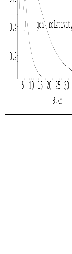
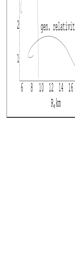
Figure 1: Total star mass $M$ versus star radius $R$. Left figure represents the Oppenheimer-Volkoff model. Right figure – the model with Tsuruta-Cameron equation of state.

This observation may be instructive for all models with dilaton fields of different kind, being under intensive investigations at present. For example, when the interaction of the dilaton field in string theories [10], [11] with the usual matter will be known, we will be able to consider a models of stars and to go to a real physics in string models.

8 The Solar System Gravitational Experiments and the Models with Torsion-Dilaton Field

Now we are ready to compare some of the models of gravity with propagating torsion under consideration with the basic gravitational experiments in solar system [36], [37]. The easiest way to do this is to use the post-Newtonian parameters [60], i.e. to obtain the asymptotic expansion of the spherically symmetric four-interval in a form:

$$ds^{2}=\left(1-{2M\over r}+2\beta{M^{2}\over r^{2}}+...\right)(c\,dt)^{2}-\left(1+2\gamma{M\over r}+...\right)\left(dr^{2}+r^{2}d\Omega^{2}\right)$$ (33)

and then to look at the coefficients $\beta$ and $\gamma$ for which at present we have tight experimental constrains [60]:

$$\mid\beta-1\mid<1*10^{-3},\mid\gamma-1\mid<2*10^{-3}.$$ (34)

8.1 The Strict Saa’s Model

In the strict Saa’s model from formula (29) we obtain the asymptotic expansion [36]:

$$ds^{2}\approx\left(1-{2M\over r}+2{M^{2}\over r^{2}}\right)(c\,dt)^{2}-\left(1+2(1-3K){M\over r}\right)\left(dr^{2}+r^{2}d\Omega^{2}\right).$$ (35)

This gives for the two post-Newtonian parameters: $\beta=1,\gamma=1-3K$. Hence, the experimental restriction on the coefficient $\beta$ is fulfilled, but the experimental restriction on the coefficient $\gamma$ leads to the requirement $\mid K\mid<{2\over 3}*10^{-3}$ which is not consistent with the theoretical prediction $K\in[{1\over 3},{1\over 2}]$ obtained for a star made from usual matter. Hence, the strict Saa’s model contradicts to the basic gravitational experiments in the solar system.

8.2 The VPC Model

Because of the different dependence of the test particles lagrangian on the torsion-dilaton field $\Theta$ [34], for a comparison of the VPC model with the solar system gravitational experiments it is convenient first to perform a conform transformation $ds^{2}\rightarrow d\!\stackrel{{\scriptstyle*}}{{s}}\!{}^{2}=e^{-6\Theta}ds^{2}$. Then the formula (29) gives the asymptotic expansion [37]:

$$d\!\stackrel{{\scriptstyle*}}{{s}}\!{}^{2}\approx\left(1-{2M\over r}+{2M^{2}\over r}\right)(c\,dt)^{2}-\left(1+{1\over 1-3K}{2M\over r}\right)\left(dr^{2}+r^{2}d\Omega^{2}\right).$$ (36)

Hence, the two post-Newtonian parameters corresponding to the effective metric $\stackrel{{\scriptstyle*}}{{g}}_{\mu\nu}$ are $\stackrel{{\scriptstyle*}}{{\beta}}=1,\,\stackrel{{\scriptstyle*}}{{\gamma}}={1\over 1-3K}$. Therefore to avoid contradictions with the basic experimental facts we must have $\left|{3K\over 1-3K}\right|<2*10^{-3}$. But the consideration of a spherically symmetric stationary star in the VPC model leads to the only possible value of the parameter $K=1$ [37]. This means that in this model the torsion part of gravitational force equals to the metric one in magnitude. As a consequence it is impossible to fulfill the second of the experimental restrictions (34). Hence, the VPC model is not consistent with the basic gravitational experiments in the solar system, too.

8.3 The Models Based on Modified Variational Principle

As we sow in the previous subsections of Section 8 both the strict Saa’s model and the VPC model have no SCMCP for fluids and particles and contradict to the experimental data. The problem with SCMCP may be solved formally making use of the Timan’s modification of the usual variational principle for particles and fluids, as explained in Section 5. Unfortunately, the simplest models described there are not studied in details at present. As we have mentioned, in these models some additional restrictions on the motion of the test particles and fluids exist. They may have an interesting physical consequences. For example, it turns out that these models do not allow a spherically symmetric stationary solutions for stars. At present it is not clear is this a good, or a bad property of these models. In principle such unusual situation may correspond to the reality: actually we do not see any star in a stationary state. All stars we know, at list radiate energy in different ways and are not in a true stationary state. It is interesting to clarify is it possible to connect this ultimate star’s radiation with the affine geometry of the space-time.

9 A Possible Realistic Model of Gravity with Propagating Torsion-Dilaton

The results we described in the previous Sections inspire further modification of the model with torsion-dilaton field.

9.1 The Action for Spinless Matter and Matter Fields.

The construction of the action for spinless matter and matter fields is based on the following facts:

1. The real success of Saa’s model with respect to the SCMCP is achieved thanks to the insertion of the factor $e^{-3\Theta}$ into the action integral for the matter fields (15). Actually for the same purpose it is enough to put this factor precisely into the corresponding kinetic part of the action integrals for matter fields.

2. The consistence requirement for the semiclassical limit dictates to put into the mass terms of the lagrangians of these fields factors of the form $e^{-p\Theta}$ with different constants $p$ for different massive fields [34] as was pointed out in the Section 2.

3. According to Kleinert and Pelster [52], the situation with SCMCP for the relativistic spinless test particles appears to be similar to the case of matter fields in Saa’s model: if the torsion is determined by torsion-dilaton field only, the A-type equation of motion (4) may be derived via the usual action principle from the modified action:

$${\cal A}_{m}[x]=-m\int e^{-\Theta}\sqrt{g_{\mu\nu}(x))dx^{\mu}dx^{\nu}}=-m\int e^{-\Theta}ds.$$ (37)

It is not hard to obtain that the action

$${\cal A}_{\mu}[x]=-\int d^{4}x\sqrt{|g|}\,e^{-\Theta}\left({\mu+\mu\Pi}\right)$$ (38)

via the usual variational principle yields precisely the A-type equations of motion (27). For this purpose one has to take into account that in Lagrange variables the fluid’s mass density is $\mu=\mu_{0}{\frac{\sqrt{g_{\mu\nu}{\dot{x}}^{\mu}{\dot{x}}^{\nu}}}{J(x)\sqrt{|g|}}}$, $J(x)$ being the Jacobian of the transition from Euler to Lagrange variables (See for details the similar calculations in [34] and the references there in).

Our SCMCP based on the combination of 1-3 gives a definite action for massive spinless matter fields when torsion is produced by torsion-dilaton field only:

$${\cal A}_{\phi}[\phi(x)]=\int d^{4}x\sqrt{|g|}\,e^{-3\Theta}\,{{\small\,\,\hbox{${\frac{1}{2}}$}}}\!\left(g^{\mu\nu}\partial_{\mu}\phi\partial_{\nu}\phi-m^{2}e^{-2\Theta}\phi^{2}\right)$$ (39)

and the A-type equation of motion:

$$\Box\phi+m^{2}e^{-2\Theta}\phi=0.$$ (40)

The semiclassical limit of this equation is

$$g^{\alpha\beta}\partial_{\alpha}\varphi\partial_{\beta}\varphi=m^{2}e^{-2\Theta}$$ (41)

and yields precisely to the Hamilton-Jacobi equation of the classical particle with action (37).

9.2 The Action for Geometric Fields.

The next problem is the construction of the action for geometric fields $g_{\alpha\beta}$ and $\Theta$. We can use the experience we gained working in the previous models of gravity with torsion-dilaton field after some important remarks.

1) It is not hard to see, that the torsion-dilaton field $\Theta$ is the only scalar field which enters in the total torsion tensor ${S_{\alpha\beta}}^{\gamma}$ of a general affine connection, being complete independent of the metric $g_{\alpha\beta}$.

2) If we wish to preserve general relativity as a right theory of the metric part of the space-time geometry we have not to destroy the metric dependence of the corresponding action. Then the only possibility is to write down this part of the action in a form

$${\cal A}_{G}[g_{\alpha\beta},{S_{\alpha\beta}}^{\gamma}]=-{\frac{1}{2\kappa}}\int\,F(\Theta)\,R\,\sqrt{|g|}d^{4}x,$$ (42)

with an arbitrary new function $F(\Theta)$. This way we worked out at the same time the action for the torsion-dilaton field $\Theta$, which enters in the Cartan curvature $R$ according to the formula $R=\stackrel{{\scriptstyle\{\}}}{{R}}+6\left({\stackrel{{\scriptstyle{}^{\{\}}}}{{\Box}}}\Theta-g^{\mu\nu}\partial_{\mu}\Theta\partial_{\nu}\Theta\right)$. In this unique situation we do not need to put by hands additional terms and coupling constants for the torsion-dilaton field $\Theta$, i.e. we have a specific form of SCMCP for the very torsion dilaton field. Hence, as in the previous models, the space-time geometry will be complete determined by the usual properties of the matter and the interaction of the matter with torsion-dilaton field is definitely determined by the geometry via SCMCP, possibly supplied by some additional requirements.

3) We know from previous considerations that the choice of the new function $F(\Theta)$ in a form $F(\Theta)=e^{-3\Theta}$ contradicts to the basic solar system gravitational experiments. Hence, a new choice of this function is needed. It cannot be derived via the SCMCP, because now we have to determine in a physically acceptable way the self-interaction of the geometrical fields $g_{\alpha\beta}$ and $\Theta$. The SCMCP gives no instructions in this direction.

a) There exists a simple choice $F(\Theta)=e^{-2\Theta}$ which yields a theory just in the spirit of string theories [10], [11]. It is very interesting to investigate such model in details. In it the string dilaton appears in the torsion, not in the Weyl’s nonmetricity as it was initially proposed in [9]. If we accept this idea then our approach has an important advantage: the geometry and the SCMCP will imply a definite interaction of the string-torsion-dilaton field with the usual matter. A nonminimal coupling of the torsion-dilaton with matter fields based on some additional principles is also possible. We have to remind the reader that the standard string theory is not able to make such predictions at present.

It is evident that if in this variant of theory we consider only geometric fields and usual matter, i.e. if the total action is ${\cal A}_{total}={\cal A}_{G}+{\cal A}_{\mu}+{\cal A}_{m}$ then in Einstein frame ($g^{\mu\nu}_{Einstein}=e^{-2\Theta}g^{\mu\nu}$) we will turn back to the usual general relativity. Hence, this variant of theory is consistent with all known gravitational experiments concerning usual matter [60]. But some new effects may emerge due to the new theory of matter fields in presence of torsion-dilaton.

b) Another very interesting possibility is to use a function $F(\Theta)\neq e^{-2\Theta}$ which is consistent with solar system experiments. One has to add that considering a pore dilatonic gravity with action (42) S. Kalyana Rama showed recently [62] that for a large class of functions $F(\Theta)$ we can reach cosmological models without singularities.

Maybe it will be possible to combine:
1) the requirement for the existence of an universal SCMCP, based on the interpretation of the dilaton field as a potential of the torsion vector;
2) the requirement for a right description of the solar system experiments which give quite strong test of any theory of gravity;
3) the conditions which lead to an absence of cosmological singularities;
and probably
4) some additional physical requirements;
and this way to obtain at the end some simple physically consistent model of gravity with propagating torsion. The results of the study of these intriguing new possibilities will be described in next papers.

Another obvious and necessary step will be the investigation of the physical relevance of other field degrees of freedom which enter in the Cartan torsion tensor and may be related with non-zero-spin matter. The corresponding considerations will be represented somewhere else.

Acknowledgments

This work has been partially supported by the Sofia University Foundation for Scientific Researches, Contract No. 245/98, and by the Bulgarian National Foundation for Scientific Researches, Contract F610/98.

The author is grateful to the leadership of the Bogoliubov Laboratory of Theoretical Physics, JINR, Dubna, Russia for hospitality and working conditions during his stay there in the summer of 1998, as far as to the organizers of the XI International Conference Problems in Quantum Field Theory, Dubna, Russia, July 13-17, 1998 for the possibility to join this Conference and to give this talk.

The author also wishes to express his thanks for the stimulating discussions of different parts of the present talk to S. Yazadjiev, T. Boyadjiev, B. M. Barbashov, V. V. Nesterenko, A. A. Zheltukhin, A. Pelster, V. de Alfaro and M. Cavaglia.

References

- [1] E. Cartan, CR Acad. Sci. 174, p. 437, 1922.
- [2] F. Hehl, P. von der Heyde, G. Kerlick, Rev. Mod. Phys. 48, p. 393, 1976.
- [3] V. Rodichev, Teoriia tiagoteniia v ortogonalnom repere, Nauka, Moskva, 1974 (in Russian).
- [4] F. Hehl, Four Lectures on Poincaré Gauge Field Theory, in Proceedings of the 6th Course of the School of Cosmology and Gravitation on Spin, Torsion, Rotation, and Supergravity, eds. P. Bergmann, V. de Sabbata, Plenum, New York, 1980.
- [5] V. de Sabbata, M. Gasperini, Introduction to Gravitation, World Scientific Publ. Co., Singapore, 1985.
- [6] D. Ivanenko, P. Pronin, G. Sardanashvili, Kalibrovochnaia teoriia gravitacii, MGU, Moskva, 1985 (in Russian).
- [7] F. Hehl, J. McCrea, E. Mielke, Y. Ne’eman, Phys. Rep. 258, p. 1, 1995.
- [8] P. West, Introduction to Supersymmetry and Supergravity, World Scientific Publ. Co., Singapore, 1986.
- [9] J. Scherk, J. H. Schwarz, Phys. Lett. B 52, p. 347, 1974.
- [10] M. Green, J. Schwarz, E. Witten, Superstring Theory, Vols. I and II, Cambridge University Press, 1987.
- [11] E. Kiritsis, Introduction to Superstring Theory, hep-th/9709062.
- [12] G. Esposito, Nuovo Cim. 105 B, p. 75, 1990.
- [13] G. Esposito, Fortsch. Phys. 40, p. 1, 1992.
- [14] Schouten J.A., Tensor Analysis for Physicists, Clarendon Press, Oxford, 1954; Ricci-Calculus, Springer, Berlin, 1954.
- [15] H. Kleinert, Gauge Fields in Condensed Matter II, Stresses and Defects, World Scientific Publ. Co., Singapore, 1989.
- [16] H. Kleinert, Path Integrals in Quantum Mechanics, Statistics, and Polymer Physics, World Scientific Publ. Co., Singapore, 1990. Second ed., 1994.
- [17] D. Gal’tsov, P. Letelier, Phys. Rev. D 47, p. 4273, 1993.
- [18] K. Tod, Clas. Quantum Grav. 11, p. 1331, 1994.
- [19] D. Edelen, Int. J. Theor. Phys. 35, p. 1315, 1994.
- [20] P. Letelier, Clas. Quantum Grav. 12, p. 471, 1995.
- [21] J. Anandan, Phys. Rev. D 53, p. 779, 1996.
- [22] E. Stiefel, G. Scheifele, Linear and Regular Celestial Mechanics, Springer, Berlin, 1971.
- [23] V. C. De Andare, J. G. Pereira, Phys. Rev. D 54, p. 4689, 1997.
- [24] V. C. De Andare, J. G. Pereira, Gen. Rel. and Grav. 30, p. 1, 1998.
- [25] V. C. De Andare, J. G. Pereira, Torsion and the Electromagnetic Field, gr-qc/9708051.
- [26] R. T. Hammond, Gen. Rel. and Grav. 26, p. 247, 1994.
- [27] R. T. Hammond, Gen. Rel. and Grav. 28, p. 749, 1996.
- [28] R. T. Hammond, Class. Quant. Grav. 13, p. 1691, 1996.
- [29] A. Saa, Mod. Phys. Lett. A8, p. 2565, 1993.
- [30] A. Saa, Mod. Phys. Lett. A9, p. 971, 1994.
- [31] A. Saa, Class. Quant. Grav. 12, L85, 1995.
- [32] A. Saa, J. Geom. and Phys. 15, p. 102, 1995.
- [33] A. Saa, Gen. Rel. and Grav. 29, p. 205, 1997.
- [34] P. Fiziev, Gen. Rel. Grav. 30, p. 1341, 1998; E-print gr-qc/9712004.
- [35] T. Boyadjiev, P. Fiziev, S. Yazadjiev Neutron star in presence of torsion-dilaton field, preprint JINR, Dubna E-98-218; E-print gr-qc/9803084.
- [36] P. Fiziev, S. Yazadjiev, Solar-system experiments and Saa’s model of gravity with propagating torsion, preprint JINR, Dubna E-98-219; E-print gr-qc/9806063.
- [37] P. Fiziev, S. Yazadjiev, Solar-system experiments and the interpretation of Saa’s model of gravity with propagating torsion as a theory with variable Planck “constant”, preprint JINR, Dubna E-98-220; E-print gr-qc/9807025.
- [38] H. Timan, Variational principle with torsion, Ingenier, 5, p. 82, 1970. Being not able to find the original of this reference we refer to it following the reference: V. G. Krechet, V. N. Ponomorev, Observable Effects of Torsion in Space-Time (Equations of Motion), in Problemi Teorii Gravitacii i Elementarnih Chastic, editor Staniukovich K.P., Atomizdat, Moskow, p. 174, 1976 (in Russian).
- [39] P. P. Fiziev, H. Kleinert, Variational Principle for Classical Particle Trajectories in Spaces with Torsion, Europhys. Lett., 35, p. 241, 1996; E-print hep-th/9503073.
- [40] P. P. Fiziev, H. Kleinert, Anholonomic Transformations in the Mechanical Variational Principle, in Proceedings of the Workshop on Variational and Local Methods in the Study of Hamiltonian Systems, editors A. Ambrosetti and G. F. Dell’Antonio, World Scientific Publ. Co., Singapore, p. 166, 1995; E-print: gr-qc/9605046.
- [41] P. P. Fiziev, On the Action Principle in Affine Flat Spaces with Torsion, in the Proceedings of the 2-nd Bulgarian Workshop ”New Trends in Quantum Field Theory”, Razlog, 1995, editors A. Ganchev, R. Kerner, I. Todorov, Heron Press Science Series, Sofia, p. 248, 1996, E-print: gr-qc/9712002.
- [42] H. Kleinert, A. Pelster, Lagrange Mechanics in Spaces with Curvature and Torsion, FU-preprint, gr-qc/9605028 .
- [43] H. Kleinert, S. V. Shabanov., Spaces with torsion from embedding and the special role of autoparallel trajectories, E-print: gr-qc/9709067.
- [44] Nuno Barros e Sá, Geodesics or autoparallels from a variational principle, preprint USTP 97-19; E-print: gr-qc/9712013.
- [45] H. Weyl, Space-Time-Matter, (fifth eddition) Springer, Berlin, 1923.
- [46] P. A. M. Dirac, The Lagrangian in Quantum mechanics, Phys. Zeit. der Sowietunion 3, p. 64, 1933.
- [47] R. P. Feynman, A. R. Hibbs, Quantum Mechanics and Path Integrals, McGrow-Hill Co., New York, 1965.
- [48] P. P. Fiziev, H. Kleinert, Comment on Path Integral Derivation of Schrödinger Equation in Spaces with Curvature and Torsion, Journal of Physics A 29, p. 7619, 1996; E-print: hep-th/9604172.
- [49] V. N. Ponomorev, Observable Effects of Torsion in Space-Time, Bull. Acad. Pol. Sci. (Math., astr., phys.) 19, p. 545, 1971.
- [50] H. Kleinert, Quantum Equivalence Principle, in Functional Integration, Basics and Applications, editors C. DeWitt-Morette, P. Cartier, A. Folacci, NATO ASI Series, Series B: Physics 361, Plenum Press, N. Y. and London, 1997.
- [51] H. Kleinert, Nonholonomic Mapping Principle for Classical Mechanics in Spaces with Curvature and Torsion. New Covariant Conservation Law for Energy-Momentum Tensor, Jadwisin Lecture Notes: APS preprint aps1997sep03_002; E-print: gr-qc/9801003.
- [52] H. Kleinert, A. Pelster, Novel Geometric Gauge Invariance of Autoparallels, gr-qc/9801030.
- [53] E. Schrödinger, Expanding Universe, Cambrige University Press, 1956.
- [54] C. Brans, R. H. Dicke, Phys. Rev. 124, p. 925, 1961.
- [55] C. Brans, Phys. Rev. 125, p. 2194, 1961.
- [56] Ya. B. Zel’dovich, Zh. Eksp. Teor. Fiz. 37, p. 569, 1961.
- [57] Ya. B. Zel’dovich, I. D. Novikov, Stars and Relativity, The University of Chicago Press, 1971.
- [58] J. R. Oppenheimer, G. M. Volkov, Phys. Rev. 55, p. 374, 1939.
- [59] S. Tsuruta, A. G. W. Cameron, Can. J. Phys. 44, p. 1895, 1966.
- [60] C. M. Will, Theory and Experiment in Gravitational Physics, Cambridge University Press, 1993.
- [61] J. D. Bekenstein, A. Meisels, Phys. Rev. D 22, p. 1313, 1980.
- [62] S. Kalyana Rama, Phys. Rev. D 56, p. 6230, 1997.