Abstract

The final fate of the spherically symmetric collapse of a perfect fluid which follows the $\gamma$-law equation of state and adiabatic condition is investigated. Full general relativistic hydrodynamics is solved numerically using a retarded time coordinate, the so-called observer time coordinate. Thanks to this coordinate, the causal structure of the resultant space-time is automatically constructed. Then, it is found that a globally naked, shell-focusing singularity can occur at the center from relativistically high-density, isentropic, and time symmetric initial data if $\gamma\lesssim 1.01$ within the numerical accuracy. The result is free from the assumption of self-similarity. The upper limit of $\gamma$ with which a naked singularity can occur from generic initial data is consistent with the result of Ori and Piran based on the assumption of self-similarity.

Department of Physics Kyoto University

KUNS 1518

Final fate of the spherically symmetric collapse of a perfect fluid

Tomohiro Harada

Department of Physics, Kyoto University, Kyoto 606-8502, Japan

I Introduction

The singularity theorem [1] predicts the existence of singularity in the generic gravitational collapse of a massive star. However it does not state whether or not the singularity is covered by a horizon. The naked singularity is considered to be harmful because it spoils the predictability of physics. Hence, Penrose [2, 3] presented a cosmic censorship hypothesis. The weak version says that all singularities are hidden in black holes. The strong version says that no singularity can be seen by any observer. We call a singularity censored by the weak version a globally naked singularity, and a singularity allowed by the weak version but censored by the strong version a locally naked singularity. Cosmic censorship has not yet been proved. In fact, we can easily find that some solutions of Einstein equation have a naked singularity. Therefore it is important to find out whether those solutions with a naked singularity are physically realizable or not. For example, we may consider that some energy condition should be imposed on physical matters. We should also give regular and generic initial data. In order to have insight into the physical reasonableness, it will be helpful to understand in what case a naked singularity appears. If a naked singularity is possible in the regime of classical gravity, we might catch a glimpse of Planck-scale high-energy physics or quantum gravity.

The spherically symmetric dust collapse is studied by many authors because of the existence of an exact solution. The collapse of a spherically symmetric and homogeneous dust ball is described by the Oppenheimer-Snyder solution. In this solution, a singularity is neither locally nor globally naked. Therefore any observer cannot see the singularity. With this solution, the usual picture of a black hole as a final fate of gravitational collapse has been generally accepted. However, once inhomogeneities of the density and velocity distributions are allowed, the above picture does not hold. In this case, the space-time is given by the Lemaître-Tolman-Bondi (LTB) solution, and it was proved that from very generic initial data the singularity can be either locally or globally naked [4, 5, 6, 7].

The assumption of pressureless matter would not be appropriate for high-density matter. It is obvious that the effect of pressure on the formation of a naked singularity should be taken into account because the formation of a naked singularity in the LTB solution results in the blow up of the density. Ori and Piran [8] investigated the collapse of a perfect fluid numerically under the assumption of self-similarity. By this assumption the equation of state of the matter is restricted to the form $p=k\rho$. They showed that a naked singularity forms if $k\lesssim 0.0105$. Analytic discussions [9] based on self-similarity followed it. An effort of getting rid of the assumption of self-similarity was made by Onozawa, Siino, and Watanabe [10]. They solved numerically the Misner-Sharp equations [11] from regular initial data and searched the formation of an apparent horizon until the density blows up and the numerical scheme breaks down. In fact, their method is not sufficient to detect naked singularities because the combination of the blow up of the density and the absence of an apparent horizon does not necessarily mean the naked singularity.

In this paper those difficulties in detection of naked singularities are avoided by constructing the null coordinate. Then, the causal structure of the space-time can be obtained automatically by solving the dynamics of the space-time and matter. Furthermore, by using the “observer time coordinates,” the coordinates never cross an event horizon and therefore the global nakedness is trivial.

We should note recent progress on the naked singularity formation in gravitational collapse. Shapiro and Teukolsky [12] showed numerically that a sufficiently prolate (even slowly rotating) spheroid of collisionless gas collapses with the blow up of the curvature invariant without the apparent horizon formation. The spherical symmetry of the LTB solution has been somewhat relaxed. It was shown that a central, shell-focusing singularity in nonspherical but quasispherical dust collapse (i.e., the Szekeres solution [13]) can be either locally or globally naked [14]. Recently the stability of the formation of the naked singularity in the LTB solution against nonspherical linear perturbations was investigated numerically, and it was suggested that the Cauchy horizon in the LTB solution is stable [15]. The restriction to matter has been relaxed to anisotropic pressure [16, 17, 18]. Harada, Iguchi, and Nakao [19] showed that the effect of rotation may induce the naked singularity formation by studying the collapse of a spherical cloud of counter-rotating particles. Choptuik [20] investigated numerically the spherically symmetric collapse of a scalar field and showed that a zero-mass black hole forms as a critical case for the black hole formation.

This paper is organized as follows. In Sec. II, the coordinate systems are presented. In Sec. III, we discuss an equation of state and initial data. In Sec. IV, the numerical results are shown. In Sec. V, we conclude the paper. We use geometrized units with $c=G=1$ throughout the paper. We follow Misner, Thorne, and Wheeler’s [21] sign conventions of the metric tensor and Riemann tensor.

II METHOD

Here we concentrate on validity of the weak cosmic censorship hypothesis, i.e., whether or not a singularity can be globally naked. The singularity is troublesome for numerical relativity because a numerical scheme breaks down at the singularity. If we choose the spacelike hypersurface as a time slice, we cannot know whether or not the singularity is naked because it depends on the further evolution of the space-time. To suggest the nakedness of the singularity, many researchers have displayed the absence of an apparent horizon. However the absence of an apparent horizon does not necessarily mean that the singularity is naked. In fact, the condition which should be imposed on time slicing in order to guarantee the singularity avoidance is not well known (for example, see Ref. [4]).

To avoid such difficulties, we adopt the time slicing more suited to determine the causal properties of the space-time. For this purpose, we use the outgoing null coordinate as a time coordinate. We determine the scaling of this null coordinate in accordance with the proper time of a distant stationary observer. This outgoing null coordinate $u$ is called the “observer time coordinate” [22]. This coordinate value corresponds to the time at which a distant observer would see the event. Hence, the observer time coordinates never cross an event horizon. The limit curve of the time slices $u=\mbox{const}$ in the limit $u\to\infty$ is, if it exists, an event horizon. Therefore, if the observer time coordinates hit a singularity, it turns out to be globally naked. The procedure to obtain a numerical solution for the space-time is as follows. First, we prepare initial data on a spacelike hypersurface $t=0$. Then, we solve the Misner-Sharp equations [11] from the initial data $t=0$ and store data on the first null ray which emanates from the center at $t=0$. When this ray reaches the stellar surface, we begin to solve the Hernandez-Misner equations [22] using the stored data on the first null ray as initial data $u=0$. See Ref. [11, 22, 23, 24] for basic equations, numerical schemes, and difference equations.

The code was tested by the collapse of a homogeneous dust ball and an inhomogeneous dust ball. A supercritical neutron star collapsed while a subcritical neutron star did not collapse within many dynamical time scales. The code was also tested by the Riemann shock tube problem and intensive explosion described by the Sedov solution. The conservation of the total mass is a good indicator of numerical errors. In all calculations presented in the next section, the total mass was conserved within the accuracy of $10^{-4}$. The artificial viscosity term may play a rather subtle role in the formation of a central singularity. To avoid such additive difficulties, this term was not included basically. Absence of this term did not spoil the results for most calculations because shock wave did not occur for most cases. Only for the cases in which the central region expanded, a shock wave occurred, and thereby the calculation suffered from serious numerical instabilities, was the artificial viscosity switched on. For those cases, the fluid did not collapse, and hence the center was regular. 2048 grid zones were prepared in most calculations.

For notational convenience, we give the expression for the line element in the coordinate systems used here. In the usual comoving coordinates, the line element is written as

$$ds^{2}=-e^{2\phi(t,A)}dt^{2}+e^{\lambda(t,A)}dA^{2}+R^{2}(t,A)d\Omega^{2},$$ (1)

while, in the observer time coordinates,

$$ds^{2}=-e^{2\psi(u,A)}du^{2}-2e^{\psi(u,A)}e^{\lambda(u,A)}dudA+R^{2}(u,A)d\Omega^{2},$$ (2)

where

$$d\Omega^{2}=d\theta^{2}+\sin^{2}\theta d\phi^{2},$$ (3)

and $A$ is chosen to be the rest-mass included within the radius $R$ in this article. In the observer time coordinates, the lapse function $e^{\psi}$ goes to zero when approaching to an event horizon. The stress-energy tensor for a perfect fluid is given as

$$T^{\mu\nu}=(\rho+p)u^{\mu}u^{\nu}+pg^{\mu\nu}.$$ (4)

III Initial Data and Equation of State

Initial data are prepared on the spacelike hypersurface in order to obtain a clear relation with physical situations. The initial data are given by the following three arbitrary functions:

$$\rho_{0}=\tilde{\rho}_{0}(R),~{}~{}e=\tilde{e}(R),~{}~{}U=\tilde{U}(R),$$ (5)

where $\rho_{0}$, $e$ are the rest-mass density and specific internal energy, respectively. $U$ is the coordinate velocity defined as

$$U\equiv e^{-\phi}\frac{\partial R}{\partial t}=e^{-\psi}\frac{\partial R}{\partial u}.$$ (6)

The total energy density is given by

$$\rho=\rho_{0}(1+e).$$ (7)

We choose the density distribution as

$$\tilde{\rho}_{0}(R) = \cases{\tilde{\rho}_{0c}\left[1-\left(\frac{R}{R_{s}}\right)^{2}\right]&($0\leq R\leq R_{s}$),\cr 0&($R_{s}<R$)\cr}.$$ (8)

The distribution of the specific internal energy and velocity is set as

$$\tilde{e}(R) = \tilde{e}_{c}\left(\frac{\tilde{\rho}_{0}}{\tilde{\rho}_{0c}}\right)^{\gamma-1},$$ (9)

$$\tilde{U}(R) = 0,$$ (10)

where $\tilde{\rho}_{0c}\equiv\tilde{\rho}_{0}(R=0)$. We use the following $\gamma$-law equation of state:

$$p=(\gamma-1)e\rho_{0}.$$ (11)

The combination of the initial data (9), equation of state (11), and adiabatic condition guarantees that pressure is in proportional to $\rho_{0}^{\gamma}$, i.e.,

$$p=K\rho_{0}^{\gamma},$$ (12)

where $K$ is constant all over the star. In this case, the initial distribution of the specific internal energy is parametrized only by the central specific internal energy $\tilde{e}_{c}$. If we take the extremely relativistic limit ($e\gg 1$), the above equation of state becomes

$$p=(\gamma-1)\rho,$$ (13)

which is the equation of state used by Ref. [8].

IV Results

In determining the final fate of collapse, here we adopt the following criteria. If the ratio of the rest-mass density of the innermost grid zone to that of the next grid zone excesses 2, we call it a central ‘singularity’ and stop the code. If the lapse function $e^{\psi}$ in the Hernandez-Misner code decreases to less than $10^{-3}$, we call it an ‘event horizon’. If a singularity occurs before an event horizon is detected, we call it a ‘naked singularity.’ The result is not so sensitive to the choice of the thresholds. Note that the blow up of the rest-mass density inevitably results in the blow up of the scalar $R^{\alpha}_{\beta}R^{\beta}_{\alpha}=64\pi^{2}(\rho^{2}+3p^{2})$. The scalar curvature $R=8\pi(\rho-3p)$ also blows up if $p\neq(1/3)\rho$.

Here, models for three values of $\tilde{e}_{c}$, $10^{2}$, $1$, and $10^{-2}$, were calculated. If $e\gtrsim 1$, then the fluid is relativistic, while, if $e\ll 1$, then the fluid is not relativistic. The results are summarized in Figs. 21–21 and Tables I–IV.

A naked singularity

First we pay attention to the naked-singular case, the model in which $\gamma-1=10^{-4}$, $\tilde{e}_{c}=10^{2}$, and $R_{s}=100M$, where $M$ is the total gravitational mass. Since the fluid is highly relativistic, the equation of state is approximately equivalent with the equation of state (13). Hence, it is expected that the feature of collapse is not sensitive to the value of $\tilde{e}_{c}$ if $\tilde{e}_{c}\gg 1$. In this calculation, the artificial viscosity was switched off. Figure 21 shows time slicing by the Misner-Sharp and Hernandez-Misner codes. The ordinate is the proper time $\tau$ of a comoving observer, and the abscissa is the circumferential radius. The Misner-Sharp slicing presented in Fig. 21 is a family of spacelike hypersurfaces $t/M=0,100,200,300,400,500,600,700,707$, where the rescaling freedom of $t$ is fixed so that $t$ agrees with the proper time at the stellar surface. On the last slice $t=707M$, the Misner-Sharp code detected a central singularity based on the criteria described above. The Hernandez-Misner slicing is a family of null hypersurfaces $u/M=0,100,200,300,400,500,600,700,728$. Also on the last slice $u=728M$, a central singularity was detected. In this figure, locations of some fluid elements are also marked. Figures 21–21 shows the Misner-Sharp time evolution of the rest-mass density $\rho_{0}$, the ratio $m/R$, and $dR/dt$ along outgoing null geodesics [which is hereafter denoted as $(dR/dt)_{ONG}$], where $m$ is the Misner-Sharp mass [11]. As seen in Fig. 21, the time evolution of the density profile in this model looks similar to the Penston’s dust collapse solution in Newtonian gravity [25] and also the LTB solution in Einstein gravity. It is remarkable that the density distribution in the central region approaches a power-law profile and therefore loses any characteristic scale. From Fig. 21, the divergent behavior of the density at the center with respect to $R$ changes at the occurrence of the singularity as

$$\rho_{0}\propto\mbox{const}\Longrightarrow\rho_{0}\propto R^{-\alpha},$$ (14)

where $\alpha\simeq 1.7$. Penston [25] showed that $\alpha=12/7$ for the dust collapse in Newtonian gravity. In the Appendix, we will show that $\alpha=12/7$ is also valid for the LTB solution on the spacelike hypersurface $t=\mbox{const}$ of the occurrence of the central singularity. As seen in Fig. 21, the ratio $m/R$ is much less than unity. This suggests that this collapse is well approximated by that in Newton gravity. The behavior of the ratio changes at the occurrence of the singularity

$$\frac{m}{R}\propto R^{2}\Longrightarrow\frac{m}{R}\propto R^{\beta},$$ (15)

where $\beta\simeq 0.3$. It should be also noted that $\beta=2/7$ in the Penston’s dust collapse solution. In the Appendix, we will show that $\beta=2/7$ for the LTB solution. Figure 21 shows that the expansion of outgoing null geodesics are always positive until the central singularity is detected. In other words, the Misner-Sharp code does not find the apparent horizon before the occurrence of the singularity. Figures 21–21 shows Hernandez-Misner time evolution of $\rho_{0}$, $m/R$, and the lapse function $e^{\psi}$. From Figs. 21 and 21, it is found that there is little difference in the divergence property of the density profile in the central region in both codes. In the Appendix, we will show that $\alpha=12/7$ and $\beta=2/7$ for the LTB solution also on the earliest null ray which emanates from the central naked singularity. Figure 21 shows that the ratio $m/R$ is much less than unity also on that null ray. In Fig. 21, it is found that $e^{\psi}$ does not vanish but remains of the order of unity until the central singularity is detected. Since $e^{\psi}$ remains of the order of unity, an event horizon has not yet formed. Figure 21 shows the growth of the central rest-mass density $\rho_{0c}$ in this model. The simulation was repeated with various radial grid resolutions. Each curve is labeled by the number of spatial grid zones used. The value of the central rest-mass density grows unboundedly. The blow up of the central rest-mass density becomes more rapid and the maximum value of it that can be attained becomes larger as the resolution becomes higher. Then, in summary, the collapse is well approximated by dust collapse both in Newton gravity and in Einstein gravity, and a central naked singularity forms in this model based on the present criteria.

B black hole

Next we take the model in which $\gamma-1=10^{-4}$, $\tilde{e}_{c}=10^{2}$, and $R_{s}=10M$ as an example of black hole formation. Also in this calculation, the artificial viscosity was switched off. Figure 21 shows time slicing by the Misner-Sharp and the Hernandez-Misner codes. The former slicing is $t/M=0,10,20,22.3$ and the latter is $u/M=0,10,20,30,40,50,60,70,72.3$. The former code was stopped because of the steepness of the density profile around the center, while the latter code was stopped because $e^{\psi}$ became less than $10^{-3}$ all over the star. The sequence of the outgoing null geodesics $u=\mbox{const}$ converges, and its limit curve is an event horizon. Figures 21–21 shows the Misner-Sharp time evolution of $\rho_{0}$, $m/R$, and $(dR/dt)_{ONG}$. The behavior of $\rho_{0}$ and $m/R$ in the central region seen in Figs. 21 and 21 is quite similar to that seen in the naked-singular case. From Fig. 21, the ratio $m/R$ is not so small although it remains less than $1/2$ which corresponds to the apparent horizon in the spherically symmetric space-time. Figure 21 shows that the Misner-Sharp code does not detect the apparent horizon until the occurrence of the central singularity although the singularity is covered by the event horizon. Figures 21–21 shows the Hernandez-Misner time evolution of $\rho_{0}$, $m/R$, and $e^{\psi}$. It is seen in Fig. 21 that the density profile around the center is not so steep even at the event horizon. The ratio $m/R$ is increased and reaches $1/2$ at the surface. Therefore the Newtonian approximation is not valid. In Fig. 21, it is shown that $e^{\psi}$ approaches zero as $u$ increases, which indicates approach to the event horizon. Figure 21 shows growth of the rest-mass density at the center for this case. The simulation was repeated with various radial grid resolutions. From this figure it would be sure that the resolution is sufficient for the following conclusion. Since the Hernandez-Misner code detects an event horizon before the occurrence of a central singularity, the singularity is covered by the event horizon. Moreover, it can be expected that this collapse would result in the locally naked singularity because the Misner-Sharp time evolution in the central region is very similar to that of the globally naked singular case.

C stable star

The final fate of collapse for $\gamma=5/3$, $\tilde{e}_{c}=10^{-2}$, and $R_{s}=100M$ is a stable star. In this calculation, the artificial viscosity was switched on in order to suppress numerical instabilities around the shock front. Figure 21 shows time slicing by both codes. The Misner-Sharp slicing is $t/M=0,2.00\times 10^{4}$, $4.00\times 10^{4}$, $6.00\times 10^{4}$, $8.00\times 10^{4}$, $1.00\times 10^{5}$, $1.20\times 10^{5}$, $1.22\times 10^{5}$. The Hernandez-Misner slicing is $u/M=0$, $2.00\times 10^{4}$, $4.00\times 10^{4}$, $6.00\times 10^{4}$, $8.00\times 10^{4}$, $1.00\times 10^{5}$, $1.18\times 10^{5}$. In this figure, it is seen that the motion of the fluid is much slower than the speed of light. Hence, the time evolutions both in the Misner-Sharp and Hernandez-Misner time slicings are basically the same. From this reason, we present here only the Misner-Sharp time evolution. Figures 21–21 show the time evolution of $\rho_{0}$, $m/R$, and $(dR/dt)_{ONG}$ respectively. In Fig. 21, it is found that the stable star has the core-envelope structure. The surface of the envelope keeps expanding, while the core is accreting the envelope. The core does not collapse but settles its density profile after many dynamical time scales. As seen in Figs. 21 and 21, the resultant core radius is about $200M$, consistent with initial total internal energy. Figure 21 shows that the Newtonian approximation is valid because the ratio $m/R$ is much less than unity. The fact that $m/R$ is proportional to $R^{-1}$ in the envelope indicates that the mass contained in the envelope is negligibly small compared to the core mass. Of course, the expansion of the outgoing null geodesics is always positive, as seen in Fig. 21. Figure 21 shows that the central region settles down after several oscillations. The simulation was repeated with various radial grid resolutions.

D parameter search

Tables I–IV summarize the final fate of collapse for $\tilde{e}_{c}=10^{2},1,10^{-2}$. Table II is the detailed search of the critical parameter region of Table I. B, N, E, BE, and SE, mean a black hole, a naked singularity, an expansion, a black hole with an envelope, and a star with an envelope, respectively. X and Y indicate some technical difficulties. X means that the present method does not work since a central singularity occurs before the first ray from the center reaches the stellar surface in the Misner-Sharp code. Y means that the stellar surface goes outward so rapidly that some numerical difficulty occurs.

From Tables I and II, we find that the final fate of collapse from less compact ($R_{s}/M\gtrsim 20$) density distribution is, in general, not a black hole but a naked singularity if the fluid is highly relativistic and $\gamma\lesssim 1.01$. The final fate of collapse from compact ($R_{s}/M\lesssim 10$) density distribution is a black hole even if the fluid is highly relativistic and $\gamma\lesssim 1.01$. If the fluid is highly relativistic and $\gamma\gtrsim 1.01$, the fluid begins to expand from less compact density distribution. It was confirmed that the above statements do not depend on details of initial density profile. From Table IV, we find that, if the fluid is not relativistic and its profile is less compact, the usual picture of collapse in Newton gravity is true. If $\gamma<4/3$, the pressure gradient cannot sustain the gravitational collapse. If $\gamma>4/3$, the final fate of collapse is a black hole, a naked singularity or a stable star depending on energetics, i.e., the total internal energy and the gravitational energy. It should be understood that, in Table IV, an N, i.e., a naked singularity means not $e\gg 1$ but only the steep density profile at the center. In fact, in the present calculation, $e$ did not become much larger than the initial value until the central singularity breaks down our numerical code because of the finite resolution. This suggests that the dynamical range of the code used here is not sufficient to recognize an N in Table IV as a genuine naked singularity. From Tables I–IV, based on the criteria described above, a naked singularity can occur from generic initial data for a relativistic perfect fluid with $\gamma\lesssim 1.01$.

V Summary and Discussions

The final fate of the spherically symmetric gravitational collapse of a perfect fluid from time-symmetric initial data has been investigated numerically. The $\gamma$-law equation of state with an adiabatic energy condition was considered. If $\gamma-1$ is small and the initial density distribution is not so compact, the collapse of a relativistic fluid results in a central, shell-focusing naked singularity. The initial data from which a naked singularity occurs is not zero-measure and therefore sufficiently generic as long as only time-symmetric and spherically symmetric initial data are considered. The final fate of a relativistic fluid is not a stable star but either a black hole or a naked singularity. This is because the total internal energy of a highly relativistic fluid dominates the gravitational energy and therefore the fluid cannot be bound. We define the critical adiabatic index $\gamma_{c}$ as an upper limit of $\gamma$ such that the collapse of highly relativistic fluid with $\gamma$ can result in the naked singularity formation from generic, time-symmetric and spherically symmetric initial data. The present numerical study shows $\gamma_{c}\simeq 1.01$.

If we consider the collapse of an unrelativistic fluid, the usual picture of the Newtonian gravity is valid. The collapse of an unrelativistic fluid with $\gamma<4/3$ does not end up with a stable star, while, for $\gamma>4/3$, a stable star is possible. The final fate of an unrelativistic fluid with $\gamma>4/3$ is basically determined by energetics. The numerical code used here cannot say whether the final fate of the collapse of an unrelativistic fluid is a black hole or a naked singularity because it needs an extremely large dynamical range.

Here we compare the results obtained here on the highly relativistic fluid with the results under the assumption of self-similarity by Ori and Piran [8]. The equations of state of both analyses are approximately common, and hence the only difference will be the genericity of initial data. The value $\gamma_{c}\simeq 1.01$ which we have obtained here agrees with the value $\gamma_{c}\simeq 1.0105$ by Ori and Piran [8] within a numerical accuracy. Note that the initial data prepared here are time symmetric while those of Ori and Piran are imploding due to the assumption of self-similarity. We should emphasize that, even with $\gamma<\gamma_{c}$, the collapse can result in either a naked singularity or a black hole and that it depends on the choice of initial data.

There is a question about whether the results obtained here support the violation of cosmic censorship. Is it possible that the adiabatic index $\gamma$ (if the adiabatic condition is a good approximation) for high-density matter is as small as $\gamma\lesssim 1.01$ ? We do not know the reason why the equation of state becomes so soft for relativistically compressed matter although we know the adiabatic index $\gamma$ may become very small and even less than unity in some unrelativistic density range [26]. For example, the radiation fluid, which is generally considered as a good approximation for relativistic matter $e\gg 1$, is given by $e=\infty$ and $\gamma=4/3$. This might be strong evidence for the validity of cosmic censorship. However, we are currently not sure of the equation of state for highly condensed matter and hence it remains an open question.

Since a space-time singularity breaks down the smoothness of physical quantities, numerical simulations cannot give a rigorous answer about the validity of cosmic censorship. Nevertheless numerical simulations give physically important possibilities about the maximum density which we can observe in principle in gravitational collapse, i.e., outside an event horizon. From this point of view, our results show that we can observe high-energy physics in gravitational collapse if the equation of state of the high-density matter is rather soft. If it is, the gravitational collapse might be a good laboratory to obtain clues about high-energy physics.

Divergent behavior at the center in the LTB solution

Here we derive the divergent behavior of a central naked singularity in the marginally bound dust collapse, which is described by the LTB solution, both on the synchronous comoving slice on which the naked singularity occurs and on the earliest null ray which emanates from the central naked singularity. For dust, the total energy density coincides with the rest-mass density identically, i.e., $\rho=\rho_{0}$. In synchronous comoving coordinates, the LTB solution of marginally bound collapse is given as

$$ds^{2} = -dt^{2}+B^{2}dr^{2}+R^{2}d\Omega^{2},$$ (16)

$$R(t,r) = \left(\frac{9F}{4}\right)^{1/3}(t_{0}(r)-t)^{2/3},$$ (17)

$$B(t,r) = R^{\prime}$$ (18)

$$\rho = \frac{1}{8\pi}\frac{F^{\prime}}{R^{2}R^{\prime}},$$ (19)

$$t_{0}(r) = \frac{2}{3\sqrt{F}}r^{3/2},$$ (20)

where the prime denotes the derivative with respect to $r$ and we set $r=R$ at $t=0$ using the rescaling freedom of $r$ in the last equation, in deriving the last equation. $F(r)$ is an arbitrary function, a half of which is the conserved Misner-Sharp mass $m(r)$. At $t=t_{0}(r)$, a singularity occurs at a mass shell labeled by $r$. Here we set $t=t_{0}(0)$ and assume analytic and generic initial data at $t=0$, i.e.,

$$\rho(t=0,r)=\rho_{0}+\rho_{2}r^{2}+\cdots,$$ (21)

where we assume that the density is a decreasing function of $r$ and therefore $\rho_{2}<0$. Then, from Eq. (19),

$$F(r)=F_{3}r^{3}+F_{5}r^{5}+\cdots,$$ (22)

where $F_{3}>0$ and $F_{5}<0$. Then, from Eqs. (17), (18), and (20) the following behavior is easily derived at $t=t_{0}(0)$ for sufficiently small $r$:

$$R \propto r^{7/3},$$ (23)

$$R^{\prime} \propto r^{4/3},$$ (24)

$$F^{\prime} \propto r^{2}.$$ (25)

From Eq. (19), we find that

$$\rho\propto r^{-4}.$$ (26)

From Eqs. (22), (23), and (26), we conclude that, at $t=t_{0}(0)$,

$$\rho \propto R^{-12/7},$$ (27)

$$\frac{m}{R} \propto R^{2/7}.$$ (28)

on the synchronous comoving slice $t=t_{0}(0)$. This behavior around the naked singularity is the same for the nonmarginally bound collapse. The blow up of the central density is given from Eqs. (17), (19), and (20) as

$$\rho(t,r=0)\propto[t_{0}(0)-t]^{-2},$$ (29)

while

$$\rho(t,r>0)\propto[t_{0}(r)-t]^{-1}.$$ (30)

Then we determine the exponents on the earliest outgoing null geodesic from the central naked singularity which results from the marginally bound dust collapse. On this null geodesic, $R$ and $R^{\prime}$ are (see, e.g. Ref. [6])

$$R \propto r^{7/3},$$ (31)

$$R^{\prime} \propto r^{4/3},$$ (32)

for $\rho(t=0,r)$ as seen in Fig. (21). Therefore, we conclude that

$$\rho \propto R^{-12/7},$$ (33)

$$\frac{m}{R} \propto R^{2/7}.$$ (34)

This behavior seen around the central naked singularity is also the same for nonmarginally bound collapse.

TABLE I.: $\tilde{e}_{c}=10^{2}$

	$\gamma-1=0$	$10^{-5}$	$10^{-4}$	$10^{-3}$	$10^{-2}$	$10^{-1}$	$1$
$R_{s}/M=10$	B	B	B	B	X	Y	Y
$50$	N	N	N	N	E	Y	Y
$100$	N	N	N	N	E	Y	Y
$1000$	N	N	N	E	E	Y	Y

TABLE II.: $\tilde{e}_{c}=10^{2}$

	$\gamma-1=2\times 10^{-3}$	$4\times 10^{-3}$	$6\times 10^{-3}$	$8\times 10^{-3}$	$10^{-2}$	$2\times 10^{-2}$
$R_{s}/M=10$	B	B	BE	X	X	X
$20$	N	N	N	N	N	BE
$30$	N	N	N	N	N	E
$40$	N	N	N	N	E	E
$50$	N	N	N	E	E	E
$60$	N	N	N	E	E	E
$70$	N	N	E	E	E	E
$80$	N	N	E	E	E	E
$90$	N	N	E	E	E	E
$100$	N	E	E	E	E	E

TABLE III.: $\tilde{e}_{c}=1$

	$\gamma-1=0$	$10^{-5}$	$10^{-4}$	$10^{-3}$	$10^{-2}$	$10^{-1}$	$1$
$R_{s}/M=10$	B	B	B	B	BE	E	E
$50$	N	N	N	N	N	E	E
$100$	N	N	N	N	E	E	E
$1000$	N	N	N	E	E	E	E

TABLE IV.: $\tilde{e}_{c}=10^{-2}$

	$\gamma-1=0$	$10^{-3}$	$10^{-2}$	$10^{-1}$	$1/3$	$2/3$	$1$
$R_{s}/M=10$	B	B	B	B	B	B	B
$50$	N	N	N	N	B	SE	SE
$100$	N	N	N	N	E	SE	SE
$1000$	N	N	N	E	E	E	E

FIGURE CAPTION

• Naked-singular model in which $\gamma-1=10^{-4}$, $\tilde{e}_{c}=10^{2}$, and $R_{s}=100M$. The slicing is by the Misner-Sharp and Hernandez-Misner codes. The ordinate is the proper time of a comoving observer, and the abscissa is the circumferential radius. The Misner-Sharp slicing is $t/M=0,100,200,300,400,500,600,700,707$ and the Hernandez-Misner slicing is $u/M=0,100,200,300,400,500,600,700,728$. The Hernandez-Misner slicing is a set of outgoing null geodesics. We stopped the calculation in both codes when we detected a central singularity. Locations of some fluid elements are marked.

• Evolution of the rest-mass density $\rho_{0}$ in the Misner-Sharp code. The density distribution in the central region at $t=707M$ becomes so steep that we call it a singularity.

• Evolution of $m/R$, the ratio of the Misner-Sharp mass to the circumferential radius, in the Misner-Sharp code.

• Evolution of $(dR/dt)_{ONG}$, $dR/dt$ along outgoing null geodesics, in the Misner-Sharp code.

• Evolution of $\rho_{0}$ in the Hernandez-Misner code. The density distribution in the central region at $u=728M$ becomes so steep that we call it a singularity.

• Evolution of $m/R$ in the Hernandez-Misner code.

• Evolution of the lapse function $e^{\psi}$ in the Hernandez-Misner code.

• Blow up of the central rest-mass density $\rho_{0c}$. The simulation was repeated with various radial grid resolutions. Each curve is labeled by the number of spatial zones used.

• Black-hole model in which $\gamma-1=10^{-4}$, $\tilde{e}_{c}=10^{2}$, and $R_{s}=10M$. The Misner-Sharp slicing is $t/M=0,10.0,20.0,22.3$. On the last slice, a singularity was detected. The Hernandez-Misner slicing is $u/M=0,10.0,20.0,30.0,40.0,50.0,60.0,70.0,72.3$. On the last slice, an event horizon was detected. The limit curve is the event horizon.

• Evolution of $\rho_{0}$ in the Misner-Sharp code. The density distribution in the central region at $t=22.3M$ becomes so steep that we call it a singularity.

• Evolution of $m/R$ in the Misner-Sharp code.

• Evolution of $(dR/dt)_{ONG}$ in the Misner-Sharp code.

• Evolution of $\rho_{0}$ in the Hernandez-Misner code. The density distribution in the central region remains not so steep even at the event horizon.

• Evolution of $m/R$ in the Hernandez-Misner code.

• Evolution of $e^{\psi}$ in the Hernandez-Misner code. The $e^{\psi}$ converges to zero as $u$ increases.

• Evolution of $\rho_{0c}$. The simulation was repeated with various radial grid resolutions. Each curve is labeled by the number of spatial zones used.

• Stable-star model in which $\gamma-1=2/3$, $\tilde{e}_{c}=10^{-2}$, and $R_{s}=100M$. The Misner-Sharp slicing is $t/M=0$, $2.00\times 10^{4}$, $4.00\times 10^{4}$, $6.00\times 10^{4}$, $8.00\times 10^{4}$, $1.00\times 10^{5}$, $1.20\times 10^{5}$, $1.22\times 10^{5}$. The Hernandez-Misner slicing is $u/M=0$, $2.00\times 10^{4}$, $4.00\times 10^{4}$, $6.00\times 10^{4}$, $8.00\times 10^{4}$, $1.00\times 10^{5}$, $1.18\times 10^{5}$.

• Evolution of $\rho_{0}$ in the Misner-Sharp code. The density distribution of the core settles down after $t\simeq 6.00\times 10^{4}$.

• Evolution of $m/R$ in the Misner-Sharp code.

• Evolution of $(dR/dt)_{ONG}$ in the Misner-Sharp code.

• Evolution of $\rho_{0c}$. The simulation was repeated with various radial grid resolutions. Each curve is labeled by the number of spatial zones used.

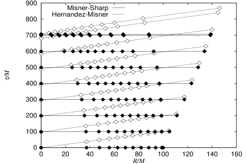
FIG. 1.:

FIG. 2.:

FIG. 3.:

FIG. 4.:

FIG. 5.:

FIG. 6.:

FIG. 7.:

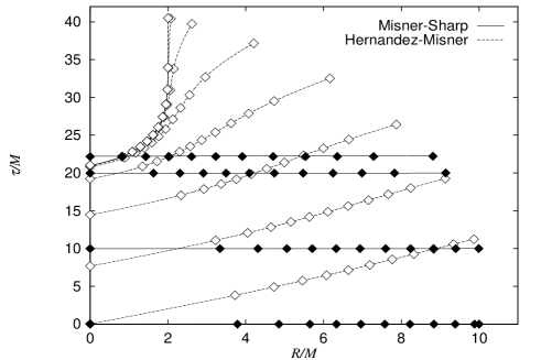
FIG. 8.:

FIG. 9.:

FIG. 10.:

FIG. 11.:

FIG. 12.:

FIG. 13.:

FIG. 14.:

FIG. 15.:

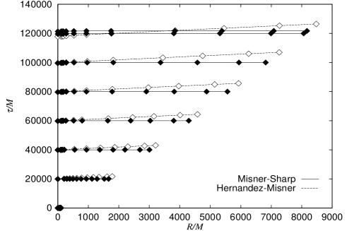
FIG. 16.:

FIG. 17.:

FIG. 18.:

FIG. 19.:

FIG. 20.:

FIG. 21.:

REFERENCES

- [1] S.W. Hawking and R. Penrose, Proc. R. Soc. Lond. A 314, 529.
- [2] R. Penrose, Riv. Nuovo Cimento I 1, 252 (1969).
- [3] R. Penrose, in General Relativity, an Einstein Centenary Survey, edited by S.W. Hawking and W. Israel (Cambridge University Press, Cambridge, England, 1979), p.581.
- [4] D.M. Eardley and L. Smarr, Phys. Rev. D 19, 2239 (1979).
- [5] D. Christodoulou, Commun. Math. Phys. 93, 171 (1984).
- [6] P.S. Joshi and I.H. Dwivedi, Phys. Rev. D 47, 5357 (1993).
- [7] T.P. Singh and P.S. Joshi, Class. Quantum Grav. 13, 559 (1996); S. Jhingan, P.S. Joshi, and T.P. Singh, ibid. 13, 3057 (1996).
- [8] A. Ori and T. Piran, Phys. Rev. Lett. 59, 2137 (1987); Gen. Relativ. Gravit. 20, 7 (1988); Phys. Rev. D 42, 1068 (1990).
- [9] P.S. Joshi and I.H. Dwivedi, Commun. Math. Phys. 146, 333 (1992); Lett. Math. Phys. 27, 235 (1993).
- [10] H. Onozawa, M. Siino, and K. Watanabe, Report No. TIT/HEP-226/COSMO-34, 1994 (unpublished).
- [11] C.W. Misner and D.H. Sharp, Phys. Rev. 136, B571 (1964).
- [12] S.L. Shapiro and S.A. Teukolsky, Phys. Rev. Lett. 66, 994 (1991); Phys. Rev. D 45, 2006 (1992).
- [13] P. Szekeres, Phys. Rev. D 12, 2941 (1975).
- [14] P.S. Joshi and A. Królak, Class. Quantum Grav. 13, 3069 (1996).
- [15] H. Iguchi, K. Nakao, and T. Harada, Phys. Rev. D 57, 7262 (1998); H. Iguchi, T. Harada, and K. Nakao, (submitted to Phys. Rev. D).
- [16] I.H. Dwivedi and P.S. Joshi, Commun. Math. Phys. 166, 117 (1994).
- [17] T.P. Singh and L. Witten, Class. Quantum Grav. 14, 3489 (1997).
- [18] G. Magli, gr-qc/9711082.
- [19] T. Harada, H. Iguchi, and K. Nakao, Phys. Rev. D 58, 041502 (1998).
- [20] M.W. Choptuik, Phys. Rev. Lett. 70, 9 (1993).
- [21] C.W. Misner, K.S. Thorne, and J.A. Wheeler, Gravitation (Freeman, New York, 1973).
- [22] W.C. Hernandez and C.W. Misner, Astrophys. J. 143, 452 (1966).
- [23] K.A. Van Riper, Astrophys. J. 232, 558 (1979).
- [24] T.W. Baumgarte, S.L. Shapiro, and S.A. Teukolsky, Astrophys. J. 443, 717 (1995).
- [25] M.V. Penston, Mon. Not. R. Astron. Soc. 144, 425 (1969).
- [26] S.L. Shapiro and S.A. Teukolsky, Black Holes, White Dwarfs, and Neutron Stars, (Wiley, New York, 1983).