Black Holes with Yang-Mills Hair

Abstract

In Einstein-Maxwell theory black holes are uniquely determined by their mass, their charge and their angular momentum. This is no longer true in Einstein-Yang-Mills theory. We discuss sequences of neutral and charged $SU(N)$ Einstein-Yang-Mills black holes, which are static spherically symmetric and asymptotically flat, and which carry Yang-Mills hair. Furthermore, in Einstein-Maxwell theory static black holes are spherically symmetric. We demonstrate that, in contrast, $SU(2)$ Einstein-Yang-Mills theory possesses a sequence of black holes, which are static and only axially symmetric.

I Introduction

The “no hair” conjecture for black holes states, that black holes are uniquely characterized by their mass, their charge and their angular momentum. This conjecture presents a generalization of rigorous results obtained for scalar fields coupled to gravity as well as for Einstein-Maxwell (EM) theory. Notably, the static black hole solutions in EM theory are spherically symmetric, and the stationary black holes are axially symmetric.

In recent years, counterexamples to the “no hair” conjecture were established in various theories with non-abelian fields, including Einstein-Yang-Mills (EYM) theory, Einstein-Yang-Mills-dilaton (EYMD) theory, Einstein-Yang-Mills-Higgs (EYMH) theory, and Einstein-Skyrme (ES) theory. These non-abelian black holes are asymptotically flat and possess a regular event horizon with non-trivial matter fields outside the event horizon.

In $SU(2)$ EYM theory, there exists a sequence of neutral static spherically symmetric non-abelian black hole solutions, labelled by the node number $n$ of the gauge field function eym . Existing for arbitrary horizon radius $x_{\rm H}$, these black hole solutions with Yang-Mills hair approach globally regular solutions bm in the limit $x_{\rm H}\rightarrow 0$. In contrast, all static spherically symmetric $SU(2)$ EYM black hole solutions with non-zero charge are embedded Reissner-Nordstrøm (RN) solutions ersh . However, this “non-abelian baldness theorem” no longer holds for $SU(3)$ EYM theory gv .

Non-abelian static spherically symmetric solutions of $SU(N)$ EYM theory are obtained by embedding the $N$-dimensional representation of $su(2)$ in $su(N)$. The gauge field ansatz then involves $N-1$ gauge field functions, and the solutions are labelled by the corresponding node numbers $(n_{1},\ldots,n_{N-1})$ kuenzle ; kks2 ; kksw ; sun . When all gauge field functions are non-trivial, neutral globally regular and black hole solutions are obtained. But when one or more of these functions are identically zero, magnetically charged black hole solutions emerge, whose charge resides in the $su(N)$ Cartan subalgebra (CSA). All these solutions possess EYMD counterparts eymd ; kks2 ; kksw ; sun .

We here first consider static spherically symmetric $SU(N)$ EYM and EYMD solutions, presenting examples of neutral globally regular $SU(4)$ solutions and charged $SU(5)$ black hole solutions, and consider also the interior of the black hole solutions.

Then we discuss globally regular and black hole solutions of $SU(2)$ EYM and EYMD theory, which are asymptotically flat, static and only axially symmetric but not spherically symmetric kk3 . These solutions are characterized by two integers, the winding number $k>1$ and the node number $n$ of the gauge field functions. The black hole solutions possess a regular event horizon and a constant surface gravity. We argue, that non-abelian theories even possess static black hole solutions with only discrete symmetries.

II $SU(N)$ EYMD action

We here consider the action of $SU(N)$ EYMD theory

$$S=\int\left(\frac{R}{16\pi G}+L_{M}\right)\sqrt{-g}d^{4}x\$$ (1)

with matter Lagrangian

$$L_{M}=-\frac{1}{2}\partial_{\mu}\Phi\partial^{\mu}\Phi-e^{2\kappa\Phi}\frac{1}{2}{\rm Tr}(F_{\mu\nu}F^{\mu\nu})\ ,$$ (2)

field strength tensor $F_{\mu\nu}=\partial_{\mu}A_{\nu}-\partial_{\nu}A_{\mu}+ie\left[A_{\mu},A_{\nu}\right]$, gauge field $A_{\mu}=\frac{1}{2}\lambda^{a}A_{\mu}^{a}$, dilaton field $\Phi$, and $e$ and $\kappa$ are the Yang-Mills and dilaton coupling constants, respectively.

III Static spherical black holes

As shown by Bartnik and McKinnon bm , $SU(2)$ EYM theory possesses a sequence of neutral globally regular solutions. These have black hole counterparts with a regular horizon eym . $SU(N)$ EYM theory possesses a with $N$ increasing number of sequences of neutral globally regular and black hole solutions kks2 ; kksw as well as of charged black hole solutions gv ; sun , which all have EYMD counterparts.

III.1 Ansätze

To construct static spherically symmetric $SU(N)$ EYM and EYMD solutions we employ Schwarzschild-like coordinates and adopt the spherically symmetric metric

$$ds^{2}=g_{\mu\nu}dx^{\mu}dx^{\nu}=-{\cal A}^{2}{\cal N}dt^{2}+{\cal N}^{-1}dr^{2}+r^{2}(d\theta^{2}+\sin^{2}\theta d\phi^{2})\ ,$$ (3)

with the metric functions ${\cal A}(r)$ and ${\cal N}(r)=1-({2m(r)}/{r})$.

The static spherically symmetric ansätze for the gauge field of $SU(N)$ EYM theory are based on the $su(2)$ subalgebras of $su(N)$. Considering the $N$-dimensional representation of $su(2)$, the ansatz is kuenzle

$$A_{\mu}^{(N)}dx^{\mu}=\frac{1}{2e}\left(\begin{array}[]{ccccc}(N-1)\cos\theta d\phi&\omega_{1}\Theta&0&\ldots&0\\ \omega_{1}\bar{\Theta}&(N-3)\cos\theta d\phi&\omega_{2}\Theta&\ldots&0\\ \vdots&&\ddots&&\vdots\\ 0&\ldots&0&\omega_{N-1}\bar{\Theta}&(1-N)\cos\theta d\phi\end{array}\right)$$ (4)

with $\Theta=id\theta+\sin\theta d\phi$, and $A_{0}=A_{r}=0$. The ansatz contains $N-1$ matter field functions $\omega_{j}(r)$. The field strength tensor component $F_{\theta\phi}$ is diagonal,

$$F_{\theta\phi}=(1/2e){\rm diag}(f_{1},...,f_{N})\sin\theta\$$ (5)

with $f_{j}=\omega_{j}^{2}-\omega^{2}_{j-1}+\delta_{j}$, $\delta_{j}=2j-N-1$ ($\omega_{0}=\omega_{N}=0$). In EYMD theory this is supplemented with the ansatz for the dilaton field, $\Phi=\Phi(r)$.

We employ the dimensionless coordinate $x=er/{\sqrt{4\pi G}}$, the dimensionless mass function $\mu=em/{\sqrt{4\pi G}}$, and the scaled matter field functions kuenzle

$$u_{j}=\frac{\omega_{j}}{\sqrt{\gamma_{j}}}\ ,\ \ \ \gamma_{j}={j(N-j)}\ ,$$ (6)

and, in EYMD theory, the dimensionless dilaton function $\varphi=\sqrt{4\pi G}\Phi$ and the dimensionless dilaton coupling constant $\gamma=\kappa/\sqrt{4\pi G}$. ($\gamma=1$ corresponds to string theory, $\gamma=0$ to EYM theory.)

III.2 Neutral solutions

When all $N-1$ gauge field functions are non-trivial, neutral solutions are obtained. The boundary conditions are chosen to have asymptotically flat solutions with a regular origin for the globally regular solutions and a regular horizon for the black hole solutions.

As an example, we consider static spherically symmetric globally regular solutions of $SU(4)$ EYM theory kksw . The $SU(4)$ EYM solutions are labelled by the node numbers $(n_{1},n_{2},n_{3})$ of the three gauge field functions $u_{1}$, $u_{2}$ and $u_{3}$, and can be classified into sequences. In Fig. 1 we present the globally regular solutions of the sequence with node structure $(n,0,0)$, $n=1-7$, with odd $n$. With increasing $n$, the solutions approach a limiting solution.

Figure 1: The matter functions $u_{1}(x)$, $u_{2}(x)$ and $u_{3}(x)$ (left) and the metric function ${\cal N}(x)$ (right) for the globally regular $SU(4)$ EYM solutions with node structure $(n,0,0)$.

To all regular solutions black hole counterparts exist. When all node numbers differ, these black hole solutions exist for arbitrary horizon radius. When two or more node numbers are the same, bifurcation phenomena occur at critical horizon radii kks2 ; kksw .

III.3 Charged solutions

When one or more of the $N-1$ gauge field functions are identically zero, magnetically charged solutions are obtained.

III.3.1 Decomposition of the ansatz

When one gauge field function is identically zero ($\omega_{j_{1}}\equiv 0$), the ansatz for the gauge field splits into two parts

$$\begin{array}[]{ccc}A_{\mu}^{(N)}dx^{\mu}&=&\left(\begin{array}[]{cc}{\rm\framebox{$A_{\mu}^{(j_{1})}dx^{\mu}$}}&\\ &{\rm\framebox{$A_{\mu}^{(N-j_{1})}dx^{\mu}$}}\\ \end{array}\right)+{\cal H}_{j_{1}}\end{array}\vspace{1.cm}\$$ (7)

with ${\cal H}_{j_{1}}=\frac{\cos\theta d\phi}{2e}h_{j_{1}}$ and

$$\begin{array}[]{ccc}{h}_{j_{1}}&=&\left(\begin{array}[]{cc}{\rm\framebox{$(N-j_{1}){\bf 1}_{(j_{1})}$}}&\\ &{\rm\framebox{$-j_{1}{\bf 1}_{(N-j_{1})}$}}\\ \end{array}\right)\\ \end{array}\vspace{1.cm}\ .$$ (8)

$A_{\mu}^{(j_{1})}$ and $A_{\mu}^{(N-j_{1})}$ denote the non-abelian spherically symmetric ansätze for the $su(j_{1})$ and $su(N-j_{1})$ subalgebras of $su(N)$ (based on the $j_{1}$ and $(N-j_{1})$-dimensional embeddings of $su(2)$, respectively), referred to by $su(\bar{N})$ in the following. ${\cal H}_{j_{1}}$ represents the ansatz for the element ${h}_{j_{1}}$ of the CSA of $su(N)$. The field strength tensor splits accordingly with

$$F^{({\cal H}_{j_{1}})}=-\frac{\sin\theta}{2e}d\theta\wedge d\phi\ h_{j_{1}}\ .$$ (9)

Considering the charge of the solution, the $su(\bar{N})$ parts of the solutions are neutral, because their field strength tensor decays at least like $O(r^{-1})$. In contrast, $F^{({\cal H}_{j_{1}})}$ does not depend on $r$. A solution based on the element $h_{j_{1}}$ of the CSA then carries charge of norm $P$,

$$P^{2}=\frac{1}{2}{\rm Tr}\ {h}_{j_{1}}^{2}\ .$$ (10)

By applying these considerations again to the subalgebras $su(\bar{N})$ of eq. (7), one obtains the general case for $SU(N)$ EYM theory sun .

RN black hole solutions exist only for horizon radius $x_{\rm H}\geq P$, and the extremal RN solution has $x_{\rm H}=P$. As first observed for $SU(3)$ EYM theory gv , the same is true for charged EYM black holes. In contrast, charged EYMD black holes exist for arbitrary $x_{\rm H}>0$, like their Einstein-Maxwell-dilaton (EMD) counterparts.

III.3.2 Extremal black hole solutions

We now apply the above general analysis to $SU(5)$ EYM theory, presenting numerical examples for the case $u_{4}\equiv 0$ sun . In that case the non-abelian part of the gauge field corresponds to an $su(4)$ part, and the solutions carry charge $P=\sqrt{10}$. In Fig. 2 and Fig. 3 (left) we present the black hole solutions of the sequence with node structure $(n,0,0)$, $n=1-7$, with odd $n$, and extremal horizon $x_{\rm H}=\sqrt{10}$, also in the interior of the black hole (for $x<x_{\rm H}$). Beside the matter function $\bar{u}_{1}$ we exhibit the charge function $P(x)$, $P^{2}(x)=2x\left(\mu(\infty)-\mu(x)\right)$ bm ; gv , and the metric function ${\cal N}(x)$.

Figure 2: The matter function $\bar{u}_{1}(x)$ (left) and the charge function $P(x)$ (right) for the $SU(4)$ EYM black hole solutions with node structure $(n,0,0)$ and extremal event horizon $x_{\rm H}=\sqrt{10}$.

Figure 3: The metric function ${\cal N}(x)$ for the $SU(4)$ EYM black hole solutions with node structure $(n,0,0)$ and extremal event horizon $x_{\rm H}=\sqrt{10}$ (left) and non-extremal event horizon $x_{\rm H}=4.5$ (right). Also shown (right) are the corresponding functions of the RN solutions with charges $P=\sqrt{10}$ and $P=4$.

III.3.3 Non-extremal black hole solutions

As seen from Fig. 2 and Fig. 3 (left), extremal EYM black hole solutions vary smoothly inside the horizon. In contrast, non-extremal EYM black hole solutions exhibit the phenomenon of mass inflation inside the horizon, analogously to neutral EYM black hole solutions massi . In Fig. 3 (right) we demonstrate this phenomenon for the metric function ${\cal N}$ for the same sequence with node structure $(n,0,0)$, $n=1-7$, $n$ odd, and non-extremal horizon $x_{\rm H}=4.5$. In contrast, for EYMD solutions with $\gamma=1$ no mass inflation occurs.

IV Static axial black holes

IV.1 Ansätze

To obtain static axially symmetric solutions, we now employ isotropic coordinates for the metric kk3 ; kk2

$$ds^{2}=-fdt^{2}+\frac{m}{f}dr^{2}+\frac{mr^{2}}{f}d\theta^{2}+\frac{lr^{2}\sin^{2}\theta}{f}d\phi^{2}\ ,$$ (11)

where $f$, $m$ and $l$ are only functions of $r$ and $\theta$. We parametrize the purely magnetic gauge field ($A_{0}=0$) by kk3 ; kk2 ; rr

$$A_{\mu}dx^{\mu}=\frac{1}{2er}\left[\tau^{k}_{\phi}\left(H_{1}dr+\left(1-H_{2}\right)rd\theta\right)-k\left(\tau^{k}_{r}H_{3}+\tau^{k}_{\theta}\left(1-H_{4}\right)\right)r\sin\theta d\phi\right]\ ,$$ (12)

with the Pauli matrices $\vec{\tau}=(\tau_{x},\tau_{y},\tau_{z})$ and $\tau^{k}_{r}=\vec{\tau}\cdot(\sin\theta\cos k\phi,\sin\theta\sin k\phi,\cos\theta)$, $\tau^{k}_{\theta}=\vec{\tau}\cdot(\cos\theta\cos k\phi,\cos\theta\sin k\phi,-\sin\theta)$, $\tau^{k}_{\phi}=\vec{\tau}\cdot(-\sin k\phi,\cos k\phi,0)$. We refer to $k$ as the winding number of the solutions. Again, the four gauge field functions $H_{i}$ and the dilaton function $\Phi$ depend only on $r$ and $\theta$. For $k=1$ the spherically symmetric ansatz of ref. eymd is recovered with $H_{1}=H_{3}=0$, $H_{2}=H_{4}=w(r)$ and $\Phi=\Phi(r)$.

Denoting the stress-energy tensor of the matter fields by $T_{\mu}^{\nu}$, with this ansatz the energy density $\epsilon=-T_{0}^{0}=-L_{M}$ becomes

$$-T_{0}^{0}= \frac{f}{2m}\left[(\partial_{r}\Phi)^{2}+\frac{1}{r^{2}}(\partial_{\theta}\Phi)^{2}\right]+e^{2\kappa\Phi}\frac{f^{2}}{2e^{2}r^{4}m}\left\{\frac{1}{m}\left(r\partial_{r}H_{2}+\partial_{\theta}H_{1}\right)^{2}\right.$$ (13)

$$+\left.\frac{k^{2}}{l}\left[\left(r\partial_{r}H_{3}-H_{1}H_{4}\right)^{2}+\left(r\partial_{r}H_{4}+H_{1}\left(H_{3}+{\rm ctg}\theta\right)\right)^{2}\right.\right.$$

$$+\left.\left.\left(\partial_{\theta}H_{3}-1+{\rm ctg}\theta H_{3}+H_{2}H_{4}\right)^{2}+\left(\partial_{\theta}H_{4}+{\rm ctg}\theta\left(H_{4}-H_{2}\right)-H_{2}H_{3}\right)^{2}\right]\right\}\ .$$

With respect to $U=e^{i\Gamma(r,\theta)\tau^{k}_{\phi}}$ the system possesses a residual abelian gauge invariance. To fix the gauge we choose the gauge condition $r\partial_{r}H_{1}-\partial_{\theta}H_{2}=0$.

IV.2 Regular solutions

We first briefly consider static axially symmetric solutions of the field equations, which have a finite mass and are globally regular and asymptotically flat.

We change to dimensionless quantities again. The dimensionless mass $\mu=(e/\sqrt{4\pi G})GM$ is determined by the derivative of the metric function $f$ at infinity, $\mu=\frac{1}{2}x^{2}\partial_{x}f|_{\infty}$. Similarly, the derivative of the dilaton function at infinity determines the dilaton charge $D=x^{2}\partial_{x}\varphi|_{\infty}$.

As for the spherically symmetric solutions, the following relations between the metric and the dilaton field hold kks2

$$\varphi(x)=\frac{1}{2}\gamma\ln(-g_{tt})\ ,$$ (14)

$$D=\gamma\mu\ .$$ (15)

For the globally regular EYM solution with $k=2$ and $n=1$ the energy density of the matter fields is shown in Fig. 4, together with a surface of constant energy density, which is toruslike.

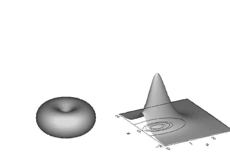
Figure 4: A surface of constant energy density (left) and the energy density (right) of the globally regular EYM solution with $k=2$ and $n=1$.

IV.3 Black hole solutions

Now we consider static axially symmetric black hole solutions with a regular event horizon. The event horizon of static black hole solutions is characterized by $g_{tt}=-f=0$. We impose that the regular horizon resides at a surface of constant $r$.

According to the zeroth law of black hole physics, the surface gravity $\kappa_{\rm sg}$ wald ; ewein ,

$$\kappa^{2}_{\rm sg}=-(1/4)g^{tt}g^{ij}(\partial_{i}g_{tt})(\partial_{j}g_{tt})\ ,$$ (16)

is constant at the horizon of the black hole solutions. It is proportional to the temperature $T=\kappa_{\rm sg}/(2\pi)$. The dimensionless area $A$ of the event horizon of the black hole solutions is proportional to the entropy $S=A/4$ wald . The black hole solutions satisfy the general mass relation

$$\mu=\mu_{\rm o}+2TS\ ,$$ (17)

with $\mu_{\rm o}=-(e/\sqrt{4\pi G})G\int_{0}^{2\pi}\int_{0}^{\pi}\int_{r_{\rm H}}^{\infty}d\phi d\theta dr\sqrt{-g}\left(2T_{0}^{\ 0}-T_{\mu}^{\ \mu}\right)$ wald , and the relation (compare (15))

$$D=\gamma(\mu-2TS)\ .$$ (18)

In Fig. 5 we exhibit surfaces of constant energy density and in Fig. 6 the energy density for the EYM black hole solution with $k=2$ and $n=1$. Also the event horizon of the black hole solutions is not spherically symmetric, but only axially symmetric kk3 .

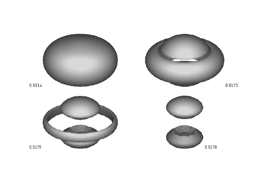
Figure 5: Surfaces of constant energy density for four values of the dimensionless energy density of the EYM black hole solution with $k=2$ and $n=1$.

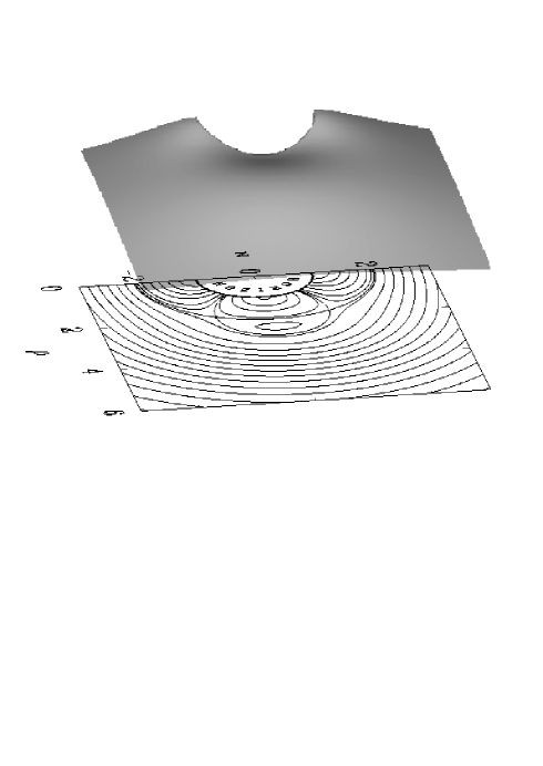
Figure 6: The energy density of the EYM black hole solution with $k=2$ and $n=1$.

V Conclusions

In EYM and EYMD theory black hole solutions are not uniquely specified by their mass, charge and angular momentum. Here we have considered static EYM and EYMD black hole solutions with non-abelian hair. The spherically symmetric solutions are unstable strau , and there is all reason to believe, that the axially symmetric black hole solutions are unstable as well. However, we expect analogous solutions in EYMH theory ewein and in ES theory, and for $n=2$ these axially symmetric black hole solutions should be stable ewein . In contrast, the stable black hole solutions with higher magnetic charges (EYMH) or higher baryon numbers (ES) should not correspond to such axially symmetric solutions with $n>2$. Instead these stable solutions should have much more complex shapes, exhibiting discrete crystal-like symmetries ewein . Analogous but unstable black hole solutions of this kind should also exist in EYM and EYMD theory.

References

- (1) Volkov, M.S., and Gal’tsov, D.V., Sov. J. Nucl. Phys. 51 747 (1990); Bizon, P., Phys. Rev. Lett. 64 2844 (1990); Künzle, H.P., and Masoud-ul-Alam, A.K.M., J. Math. Phys. 31 928 (1990).
- (2) Bartnik, R., and McKinnon, J., Phys. Rev. Lett. 61 141 (1988).
- (3) Gal’tsov, D.V., and Ershov, A.A., Phys. Lett. A138 160 (1989); Bizon, P., and Popp, O.T., Class. Quantum Grav. 9 193 (1992).
- (4) Gal’tsov, D.V., and Volkov, M.S., Phys. Lett. B274 173 (1992).
- (5) Künzle, H.P., Comm. Math. Phys. 162 371 (1994).
- (6) Kleihaus, B., Kunz, J., and Sood, A., Phys. Lett. B354 240 (1995); Phys. Lett. B374 289 (1996); Phys. Rev. D54 5070 (1996).
- (7) Kleihaus, B., Kunz, J., Sood, A., and Wirschins, M., Phys. Rev. D in press.
- (8) Kleihaus, B., Kunz, J., and Sood, A., Phys. Lett. B418 284 (1998).
- (9) Donets, E.E., and Gal’tsov, D.V., Phys. Lett. B302 411 (1993); Lavrelashvili, G., and Maison, D., Nucl. Phys. B410 407 (1993).
- (10) Kleihaus, B., and Kunz, J., Phys. Rev. Lett. 79 1595 (1997); Phys. Rev. D57 6138 (1998).
- (11) Gal’tsov, D.V., Donets, E.E., and Zotov, M.Yu., Phys. Rev. D56 3459 (1997); JETP Lett. 65 895 (1997); Breitenlohner, P., Lavrelashvili, G., and Maison, D., Nucl. Phys. B524 427 (1998); gr-qc/9708036; Sarbach, O., Straumann, N., and Volkov, M.S., gr-qc/9709081.
- (12) Kleihaus, B., and Kunz, J., Phys. Rev. Lett. 78 2527 (1997); Phys. Rev. D57 6138 (1998).
- (13) Rebbi, C., and Rossi, P., Phys. Rev. D22 2010 (1980).
- (14) Wald, R.M., General Relativity, Chicago: University of Chicago Press, 1984.
- (15) Ridgway, S.A., and Weinberg, E.J., Phys. Rev. D52 3440 (1995).
- (16) Straumann, N., and Zhou, Z.H., Phys. Lett. B243 33 (1990).