Global Structure of Evaporating Black Holes

Abstract

By extending the charged Vaidya metric to cover all of spacetime, we obtain a Penrose diagram for the formation and evaporation of a charged black hole. In this construction, the singularity is time-like. The entire spacetime can be predicted from initial conditions if boundary conditions at the singularity are known.

PACS: 04.70.Dy, 04.20.Gz, 04.60.-m, 04.40.Nr

I Introduction

It is challenging to envision a plausible global structure for a spacetime containing a decaying black hole. If information is not lost in the process of black hole decay, then the final state must be uniquely determined by the initial state, and vice versa. Thus a post-evaporation space-like hypersurface must lie within the future domain of dependence of a pre-evaporation Cauchy surface. One would like to have models with this property that support approximate (apparent) horizons.

In addition, within the framework of general relativity, one expects that singularities will form inside black holes [1]. If the singularities are time-like, one can imagine that they will go over into the world-lines of additional degrees of freedom occurring in a quantum theory of gravity. Ignorance of the nature of these degrees of freedom is reflected in the need to apply boundary conditions at such singularities. (On the other hand, boundary conditions at future space-like singularities represent constraints on the initial conditions; it is not obvious how a more complete dynamical theory could replace them with something more natural.)

In this paper, we use the charged Vaidya metric to obtain a candidate macroscopic Penrose diagram for the formation and subsequent evaporation of a charged black hole, thereby illustrating how predictability might be retained. We do this by first extending the charged Vaidya metric past its coordinate singularities, and then joining together patches of spacetime that describe different stages of the evolution.

II Extending the Charged Vaidya Metric

The Vaidya metric [2] and its charged generalization [3, 4] describe the spacetime geometry of unpolarized radiation, represented by a null fluid, emerging from a spherically symmetric source. In most applications, the physical relevance of the Vaidya metric is limited to the spacetime outside a star, with a different metric describing the star’s internal structure. But black hole radiance [5] suggests use of the Vaidya metric to model back-reaction effects for evaporating black holes [6, 7] all the way upto the singularity.

The line element of the charged Vaidya solution is

$$ds^{2}=-\left(1-{2M(u)\over r}+{Q^{2}(u)\over r^{2}}\right)du^{2}-2\,du\,dr+r^{2}\left(d\theta^{2}+\sin^{2}\theta d\phi^{2}\right)\;.$$ (1)

The mass function $M(u)$ is the mass measured at future null infinity (the Bondi mass) and is in general a decreasing function of the outgoing null coordinate, $u$. Similarly, the function $Q(u)$ describes the charge, measured again at future null infinity. When $M(u)$ and $Q(u)$ are constant, the metric reduces to the stationary Reissner-Nordström metric. The corresponding stress tensor describes a purely electric Coulomb field,

$$F_{ru}=+{Q(u)\over r^{2}}\;,$$ (2)

and a null fluid with current

$$k_{a}=k\nabla_{a}u\;,\;\;k^{2}=+{1\over 4\pi r^{2}}{\partial\over\partial u}\left(-M+{Q^{2}\over 2r}\right)\;.$$ (3)

In particular,

$$T_{uu}={1\over 8\pi r^{2}}\left[\left(1-{2M(u)\over r}+{Q^{2}(u)\over r^{2}}\right){Q^{2}(u)\over r^{2}}+{1\over r}{\partial Q^{2}(u)\over\partial u}-2{\partial M(u)\over\partial u}\right]\;.$$ (4)

Like the Reissner-Nordström metric, the charged Vaidya metric is beset by coordinate singularities. It is not known how to remove these spurious singularities for arbitrary mass and charge functions (for example, see [9]). We shall simply choose functions for which the relevant integrations can be done and continuation past the spurious singularities can be carried out, expecting that the qualitative structure we find is robust.

Specifically, we choose the mass to be a decreasing linear function of $u$, and the charge to be proportional to the mass:

$$M(u)\equiv au+b\equiv\tilde{u}\;,\;\;Q(u)\equiv\eta\tilde{u}\;,$$ (5)

where $a<0$ and $|\eta|\leq 1$, with $|\eta|=1$ at extremality. We always have $\tilde{u}\geq 0$. With these choices, we can find an ingoing (advanced time) null coordinate, $v$, with which the line element can be written in a “double-null” form:

$$ds^{2}=-{g(\tilde{u},r)\over a}d\tilde{u}\,dv+r^{2}\left(d\theta^{2}+\sin^{2}\theta d\phi^{2}\right)\;.$$ (6)

Thus

$$dv={1\over g(\tilde{u},r)}\left[\left(1-{2\tilde{u}\over r}+{\eta^{2}\tilde{u}^{2}\over r^{2}}\right){d\tilde{u}\over a}+2\,dr\right]\;.$$ (7)

The term in brackets is of the form $X(\tilde{u},r)\,d\tilde{u}+Y(\tilde{u},r)\,dr$. Since $X(\tilde{u},r)$ and $Y(\tilde{u},r)$ are both homogeneous functions, Euler’s relation provides the integrating factor: $g(\tilde{u},r)=X(\tilde{u},r)\tilde{u}+Y(\tilde{u},r)r$. Hence

$${\partial v\over\partial r}=\frac{r^{2}}{r^{3}+{\tilde{u}\over 2a}(r^{2}-2\tilde{u}r+\eta^{2}\tilde{u}^{2})}$$ (8)

$${\partial v\over\partial\tilde{u}}=\frac{{1\over 2a}(r^{2}-2\tilde{u}r+\eta^{2}\tilde{u}^{2})}{r^{3}+{\tilde{u}\over 2a}(r^{2}-2\tilde{u}r+\eta^{2}\tilde{u}^{2})}\;.$$ (9)

From the sign of the constant term of the cubic, we know that there is at least one positive zero. Then, calling the largest positive zero $r^{\prime}$, we may factorize the cubic as $(r-r^{\prime})(r^{2}+\beta r+\gamma)$. Hence

$$\gamma=-{\eta^{2}\tilde{u}^{3}\over 2ar^{\prime}}>0\;,\;\;\gamma-\beta r^{\prime}=-{\tilde{u}^{2}\over 2a}>0\;,\;\;\beta-r^{\prime}={\tilde{u}\over 2a}<0\;.$$ (10)

Consequently, the cubic can have either three positive roots, with possibly a double root but not a triple root, or one positive and two complex (conjugate) roots. We consider these in turn.

i) Three positive roots

When there are three distinct positive roots, the solution to Eq. (8) is

$$v=A\ln(r-r^{\prime})+B\ln(r-r_{2})+C\ln(r-r_{1})\;,$$ (11)

where $r^{\prime}>r_{2}>r_{1}>0$, and

$$A={+{r^{\prime}}^{2}\over(r^{\prime}-r_{2})(r^{\prime}-r_{1})}>0\;,\;\;B={-{r_{2}}^{2}\over(r^{\prime}-r_{2})(r_{2}-r_{1})}<0\;,\;\;C={+{r_{1}}^{2}\over(r^{\prime}-r_{1})(r_{2}-r_{1})}>0\;.$$ (12)

We can push through the $r^{\prime}$ singularity by defining a new coordinate,

$$V_{2}(v)\equiv e^{v/A}=(r-r^{\prime})(r-r_{2})^{B/A}(r-r_{1})^{C/A}\;,$$ (13)

which is regular for $r>r_{2}$. To extend the coordinates beyond $r_{2}$ we define

$$V_{1}(v)\equiv k_{2}+(-V_{2})^{A/B}=k_{2}+(r^{\prime}-r)^{A/B}(r_{2}-r)(r-r_{1})^{C/B}\;,$$ (14)

where $k_{2}$ is some constant chosen to match $V_{2}$ and $V_{1}$ at some $r^{\prime}>r>r_{2}$. $V_{1}(r)$ is now regular for $r_{2}>r>r_{1}$. Finally, we define yet another coordinate,

$$V(v)\equiv k_{1}+(-(V_{1}-k_{2}))^{B/C}=k_{1}+(r^{\prime}-r)^{A/C}(r_{2}-r)^{B/C}(r-r_{1})\;,$$ (15)

which is now free of coordinate singularities for $r<r_{2}$. A similar procedure can be applied if the cubic has a double root.

ii) One positive root

When there is only one positive root, $v$ is singular only at $r=r^{\prime}$:

$$v=A\ln(r-r^{\prime})+{1\over 2}B\ln(r^{2}+\beta r+\gamma)+\frac{2C-B\beta}{\sqrt{4\gamma-\beta^{2}}}\arctan\left(\frac{2r+\beta}{\sqrt{4\gamma-\beta^{2}}}\right)\;.$$ (16)

We can eliminate this coordinate singularity by introducing a new coordinate

$$V(v)\equiv e^{v/A}=(r-r^{\prime})(r^{2}+\beta r+\gamma)^{B/2A}\exp\left[+{2C-B\beta\over A\sqrt{4\gamma-\beta^{2}}}\arctan\left(\frac{2r+\beta}{\sqrt{4\gamma-\beta^{2}}}\right)\right]\;,$$ (17)

which is well-behaved everywhere. The metric now reads

$$ds^{2}=-g(\tilde{u},r){A\over V(\tilde{u},r)}\,{d\tilde{u}\over a}\,dV+r^{2}d\Omega^{2}\;.$$ (18)

In all cases, to determine the causal structure of the curvature singularity we express $dV$ in terms of $du$ with $r$ held constant. Now we note that, since $\tilde{u}$ is the only dimensionful parameter, all derived dimensionful constants such as $r^{\prime}$ must be proportional to powers of $\tilde{u}$. For example, when there is only positive zero, Eq. (17) yields

$$\left.dV\right|_{r}=d\tilde{u}\,{V\over\tilde{u}}\left[{-r^{\prime}\over r-r^{\prime}}+{B\over 2A}{\beta r+2\gamma\over r^{2}+\beta r+\gamma}+{2C-B\beta\over A\sqrt{4\gamma-\beta^{2}}}{1\over 1+\left(\frac{2r+\beta}{\sqrt{4\gamma-\beta^{2}}}\right)^{2}}{-2r\over{\sqrt{4\gamma-\beta^{2}}}}\right]\;.$$ (19)

Thus, as $r\rightarrow 0$, and using the fact that $A+B=1$, we have

$$ds^{2}\rightarrow-{Q^{2}(u)\over r^{2}}\,du^{2}\;,$$ (20)

so that the curvature singularity is time-like.

III Patches of Spacetime

Our working hypothesis is that the Vaidya spacetime, since it incorporates radiation from the shrinking black hole, offers a more realistic background than the static Reissner spacetime, where all back-reaction is ignored. In this spirit, we can model the black hole’s evolution by joining patches of the collapse and post-evaporation (Minkowski) phases onto the Vaidya geometry.

To ensure that adjacent patches of spacetime match along their common boundaries, we can calculate the stress-tensor at their (light-like) junction. The absence of a stress-tensor intrinsic to the boundary indicates a smooth match when there is no explicit source there. Surface stress tensors are ordinarily computed by applying junction conditions relating discontinuities in the extrinsic curvature; the appropriate conditions for light-like shells were obtained in [8]. However, we can avoid computing most of the extrinsic curvature tensors by using the Vaidya metric to describe the geometry on both sides of a given boundary, because the Reissner-Nordström and Minkowski spacetimes are both special cases of the Vaidya solution.

Initially then, we have a collapsing charged spherically symmetric light-like shell. Inside the shell, region I, the metric must be that of flat Minkowski space; outside, region II, it must be the Reissner-Nordström metric, at least initially. In fact, we can describe both regions together by a time-reversed charged Vaidya metric,

$$ds^{2}=-\left(1-{2M(v)\over r}+{Q^{2}(v)\over r^{2}}\right)dv^{2}+2\,dv\,dr+r^{2}d\Omega^{2}\;,$$ (21)

where the mass and charge functions are step functions of the ingoing null coordinate:

$$M(v)=M_{0}\Theta(v-v_{0})\;,\;\;Q(v)=\eta M(v)\;.$$ (22)

The surface stress tensor, $t^{s}_{vv}$, follows from Eq. (4). Thus

$$t^{s}_{vv}={1\over 4\pi r^{2}}\left(M_{0}-{Q^{2}_{0}\over 2r}\right)\;.$$ (23)

The shell, being light-like, is constrained to move at 45 degrees on a conformal diagram until it has collapsed completely. Inside the shell, the spacetime is guaranteed by Birkhoff’s theorem to remain flat until the shell hits $r=0$, at which point a singularity forms.

Meanwhile, outside the shell, we must have the Reissner-Nordström metric. This is appropriate for all $r>r_{+}$. Once the shell nears $r_{+}$, however, one expects that quantum effects start to play a role. For non-extremal ($|\eta|<1$) shells, the Killing vector changes character – time-like to space-like – as the apparent horizon is traversed, outside the shell. This permits a virtual pair, created by a vacuum fluctuation just outside or just inside the apparent horizon, to materialize by having one member of the pair tunnel across the apparent horizon. Thus, Hawking radiation begins, and charge and energy will stream out from the black hole.

We shall model this patch of spacetime, region III, by the Vaidya metric. This must be attached to the Reissner metric, region II, infinitesimally outside $r=r_{+}$. A smooth match requires that there be no surface stress tensor intrinsic to the boundary of the two regions. The Reissner metric can be smoothly matched to the radiating solution along the $u=0$ boundary if $b=M_{0}$ in Eq. (5).

Now, using Eqs. (7) and (17), one can write the Vaidya metric as

$$ds^{2}=-{g^{2}(\tilde{u},r)A\over\left(1-{2M(u)\over r}+{Q^{2}(u)\over r^{2}}\right)V^{2}}\,dV^{2}+2{g(\tilde{u},r)A\over\left(1-{2M(u)\over r}+{Q^{2}(u)\over r^{2}}\right)V}\,dV\,dr\;.$$ (24)

We shall assume for convenience that $g(r)$ has only one positive real root, which we call $r^{\prime}$. Then, since $V$ and $g$ both contain a factor $(r-r^{\prime})$, Eq. (17), the above line element and the coordinates are both well-defined for $r>r_{+}(\tilde{u})$. In particular, $r=\infty$ is part of the Vaidya spacetime patch. Moreover, the only solution with $ds^{2}=dr=0$ also has $dV=0$, so that there are no light-like marginally trapped surfaces analogous to the Reissner $r_{\pm}$. In other words, the Vaidya metric extends to future null infinity, ${\cal I}^{+}$, and hence there is neither an event horizon, nor a second time-like singularity on the right of the conformal diagram.

The singularity on the left exists until the radiation stops, at which point one has to join the Vaidya solution to Minkowski space. This is easy: both spacetimes are at once encompassed by a Vaidya solution with mass and charge functions

$$M(u)=(au+b)\Theta(u_{0}-u)\;,\;\;Q(u)=\eta M(u)\;.$$ (25)

As before, the stress tensor intrinsic to the boundary at $u_{0}$ can be read off Eq. (4):

$$t^{s}_{uu}={1\over 4\pi r^{2}}\left[(au+b)-{(au+b)^{2}\over 2r}\right]\;,$$ (26)

which is zero if $u_{0}=-b/a$, i.e., if $\tilde{u}=0$. This says simply that the black hole must have evaporated completely before one can return to flat space.

Collecting all the constraints from the preceding paragraphs, we can put together a possible conformal diagram, as in Fig. 1. (We say “possible” because a similar analysis for an uncharged hole leads to a space-like singularity; thus our analysis demonstrates the possibility, but not the inevitability, of the behaviour displayed in Fig. 1.) Fig. 1 is a Penrose diagram showing the global structure of a spacetime in which a charged imploding null shock wave collapses catastrophically to a point and subsequently evaporates completely. Here regions I and IV are flat Minkowski space, region II is the stationary Reissner-Nordström spacetime, and region III is our extended charged Vaidya solution. The zigzag line on the left represents the singularity, and the straight line separating region I from regions II and III is the shell. The curve connecting the start of the Hawking radiation to the end of the singularity is $r_{+}(\tilde{u})$, which can be thought of as a surface of pair creation. The part of region III interior to this line might perhaps be better approximated by an ingoing negative energy Vaidya metric.

From this cut-and-paste picture we see that, given some initial data set, only regions I and II and part of region III can be determined entirely; an outgoing ray starting at the bottom of the singularity marks the Cauchy horizon for these regions. Note also that there is no true horizon; the singularity is naked. However, because the singularity is time-like, Fig. 1 has the attractive feature that predictability for the entire spacetime is restored if conditions at the singularity are known. It is tempting to speculate that, with higher resolution, the time-like singularity might be resolvable into some dynamical Planck-scale object such as a D-brane.

Acknowledgement

F.W. is supported in part by DOE grant DE-FG02-90ER-40542.

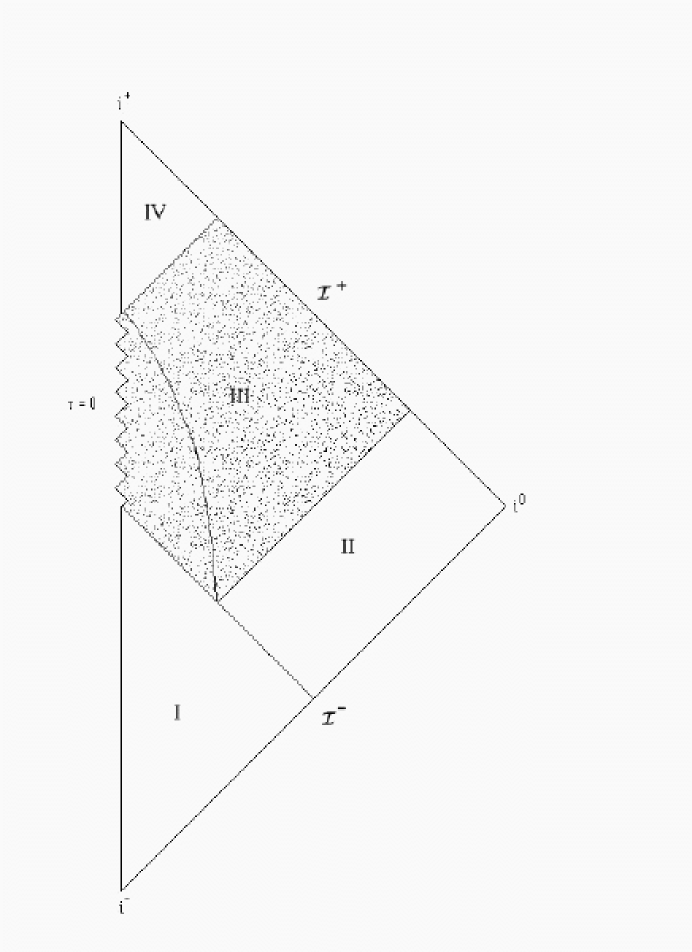
Fig. 1.: Penrose diagram for the formation and evaporation of a charged black hole.

REFERENCES

- [1] R. Penrose, Phys. Rev. Letts. 14 (1965) 57.
- [2] P.C. Vaidya, Proc. Indian Acad. Sci. A 33 (1951) 264.
- [3] J. Plebanski, J. Stachel, J. Math. Phys. 9 (1967) 269.
- [4] W.B. Bonnor, P.C. Vaidya, Gen. Rel. and Grav. 1 (1970) 127.
- [5] S.W. Hawking, Commun. Math. Phys. 43 (1975) 199.
- [6] W.A. Hiscock, Phys. Rev. D 23 (1981) 2823.
- [7] R. Balbinot, in: R. Ruffini (Ed.), Proceedings of the Fourth Marcel Grossmann Meeting on General Relativity, 1988, North-Holland, Amsterdam, p. 713.
- [8] C. Barrabès, W. Israel, Phys. Rev. D 43 (1991) 1129.
- [9] F. Fayos, M.M. Martin-Prats, J.M.M. Senovilla, Class. Quant. Grav. 12 (1995) 2565.