Numerical evolution of matter in dynamical axisymmetric black hole spacetimes. I. Methods and tests

Abstract

We have developed a numerical code to study the evolution of self-gravitating matter in dynamic black hole axisymmetric spacetimes in general relativity. The matter fields are evolved with a high-resolution shock-capturing scheme that uses the characteristic information of the general relativistic hydrodynamic equations to build up a linearized Riemann solver. The spacetime is evolved with an axisymmetric ADM code designed to evolve a wormhole in full general relativity. We discuss the numerical and algorithmic issues related to the effective coupling of the hydrodynamical and spacetime pieces of the code, as well as the numerical methods and gauge conditions we use to evolve such spacetimes. The code has been put through a series of tests that verify that it functions correctly. Particularly, we develop and describe a new set of testbed calculations and techniques designed to handle dynamically sliced, self-gravitating matter flows on black holes, and subject the code to these tests. We make some studies of the spherical and axisymmetric accretion onto a dynamic black hole, the fully dynamical evolution of imploding shells of dust with a black hole, the evolution of matter in rotating spacetimes, the gravitational radiation induced by the presence of the matter fields and the behavior of apparent horizons through the evolution.

I Introduction

A Overview

An accurate description of the evolution of matter in a fully dynamical spacetime in complete generality is a longstanding and still unresolved problem in numerical relativistic astrophysics. With many important problems in urgent need of study, such as multidimensional core collapse, neutron star collisions or black hole formation, this outstanding problem represents a major gap in our ability to understand some of the most highly energetic processes in relativistic astrophysics. Numerous attempts have been made to develop such capabilities over the years, but only the spherical case can be considered essentially solved [1, 2, 3, 4, 5, 6, 7, 8], and even there it has not yet been widely applied. In higher dimensions, most of the studies have been restricted to the axisymmetric two dimensional (2D) case, and there much of the work has been devoted to hydrodynamical integrations on fixed general relativistic backgrounds[9, 10, 11, 12, 13]. Even in axisymmetry, only a few attempts have been made to consider a fully self-gravitating, dynamic background [14, 15, 16, 17]. The three-dimensional case is also being studied, but the number of fully relativistic simulations is even smaller, with only a handful of fixed background hydrodynamical codes [18, 19] and fully self-gravitating codes [20] developed to date. In view of the difficulty of a fully relativistic treatment, approximations to a complete general relativistic approach are also being developed recently [21, 22].

The reasons for the reduced number of multidimensional (2D and 3D) computations are diverse, but we can enumerate the two most obvious ones: first, the inherent difficulties and complexities of the system of equations to integrate, the Einstein field equations coupled to the general relativistic hydrodynamic equations, which make this computation one of the most challenging ones in physics. Second, the immense computational resources needed to integrate the equations for 3D evolutions were not available in the past and are only starting to be achieved at present.

B Axisymmetric General Relativistic Hydrodynamics

In the axisymmetric case there exist a number of interesting astrophysical applications that can be addressed numerically, such as the rotational collapse of stellar cores in the supernova explosion scenario, the implosion of matter shells onto a black hole, the dynamics and stability of accretion disks or the fully dynamical spacetime version of the so-called relativistic Bondi-Hoyle accretion onto a moving black hole. Some of these problems have already tentatively been studied in the past within the framework of general relativity (see references below) although many scenarios still await for first (and detailed) computations. In this paper we take some early steps on that direction focusing on the methodology we will be using in the future for the study of those systems.

In addition to the aforementioned scenarios, one of the most interesting systems to consider is the head-on collision of a neutron star with a black hole. The correct understanding of this simplified head-on model will undoubtedly serve as an important testbed for future three-dimensional codes. Hence, it is an important step that will aid in development of simulations of more complex scenarios, such as the coalescence and merging of spiral compact binaries. These catastrophic events are believed to be among the most promising sources of gravitational radiation to be detected by the gravitational wave interferometers to be operating around the turn of the century (LIGO, VIRGO, TAMA, GEO600).

The use of general relativistic axisymmetric codes in numerical relativity has been largely devoted to the study of the gravitational collapse and bounce of a rotating stellar core and the subsequent emission of gravitational radiation. These investigations started with the work of Nakamura  [14], who was the first to calculate a general relativistic rotating stellar collapse. In his calculation, he was able to track the evolution of matter and the formation of a black hole but the scheme was not accurate enough to compute the emitted gravitational radiation. Later, Stark and Piran [15] revisited this problem studying the collapse of rotating relativistic polytropic stars to black holes and succeeded in computing the gravitational radiation emission. Their code used the radial gauge and a mixture of polar and maximal slicing. The hydrodynamic equations were solved with standard finite difference methods with artificial viscosity [23, 24]. Evans [16] also studied the gravitational collapse problem but for non-rotating matter configurations. His numerical scheme to treat the matter fields was more sophisticated than previous approaches as it included monotonic upwind reconstruction procedures and flux limiters. Evans [16] was able to show that Newtonian gravity and the quadrupole formula for gravitational radiation were inadequate to study the problem. More recently, Abrahams et al. [17] have solved the Einstein equations numerically for rotating spacetimes where the source of the gravitational field is a configuration of collisionless (dust) particles. They used the code to evaluate the stability of polytropic and toroidal star clusters. Because they did not have to take pressure forces into account, they could reduce the hydrodynamic computation to a straightforward integration of the geodesic equations.

On the other hand, a few groups have concentrated on building codes to handle dynamical, axisymmetric gravitational fields in vacuum, without the complications of the matter fields. These have been applied notably to the collapse of gravitational waves to form a black hole [25, 26] and to the evolution of distorted, rotating, and colliding black holes [27, 28, 29, 30]. But, even without the presence of matter fields, these calculations have proven very difficult for a number of reasons, not the least of which are the choice of appropriate gauge conditions and the presence of numerical instabilities encountered near the axis of symmetry. These are among the reasons that work in this area has been fairly limited.

C Our proposal

We have embarked on a program to develop a series of fully relativistic codes to solve the coupled set of equations in multiple dimensions. This work builds on some years of experience in dynamic vacuum relativity (see, for example [31, 32, 33, 34, 35]) and in fixed background general relativistic hydrodynamics (see [36, 12, 13, 37]). In spherical symmetry, we have developed a code[38, 39] exploiting advances in hyperbolic treatments of both general relativistic hydrodynamics [12] and the Einstein equations themselves [40, 41]. In the 3D case, a code is under development specifically for the study of neutron star collisions [35, 42, 43].

In the present paper we report first results obtained with a 2D axisymmetric numerical code designed to evolve rotating black hole spacetimes with self-gravitating matter. We believe that this code can have a number of interesting applications in the numerical modeling of accretion processes in black hole astrophysics. In addition, it will provide important testbeds for fully 3D codes now under development. This axisymmetric code is the result of the coupling of two previously developed production codes: an advanced general relativistic hydrodynamical code for stationary spacetimes and an axisymmetric black hole code to solve the dynamic Einstein field equations in vacuum. The integration of the different variables, spacetime and hydrodynamical quantities, is, hence, performed with a unique code. The two basic building blocks of the new code are extensively described in previous work [12, 44, 31, 32].

The equations of general relativistic hydrodynamics are integrated with a modern high-resolution shock-capturing numerical scheme which relies on the knowledge of the characteristic information of the system of equations in order to build up a Riemann solver. These equations have been recently written as a hyperbolic system of conservation laws (with sources) for a general $\{3+1\}$ metric [12]. The characteristic information of the system has been explicitly obtained. The Jacobian matrices are found to have real eigenvalues and a complete set of right-eigenvectors, therefore satisfying the definition of hyperbolicity [45]. The use of these methods, also referred to as Godunov-type methods (after the seminal idea by Godunov [46]) is becoming more important in recent years, due to a number of nice properties that other finite difference methods do not share (e.g., artificial viscosity methods). Those include a consistent treatment of discontinuous solutions (shock-capturing property) combined with being high-order methods in regions where the numerical solution is smooth. Recently, the use of these methods in relativistic hydrodynamics has permitted, for the first time, an accurate description of ultrarelativistic flows in different astrophysical scenarios (see, e.g., [13],[47] and references therein).

The black hole piece of the code was originally developed by Brandt and Seidel [31, 32] and is based on the standard Arnowitt-Deser-Misner (ADM) [48] formulation of the Einstein equations as an initial value (or Cauchy) problem. The metric and extrinsic curvature components are evolved for the full set of the Einstein equations using a $\{3+1\}$ explicit second order Runge-Kutta scheme with centered differencing. This code has a black hole built into the initial hypersurface of the spacetime. This avoids possible coordinate problems at the origin of the spherical coordinate system, since the black hole is constructed with an isometry that maps its interior, which contains a singularity at the origin, to the exterior, across a sphere at a finite radius. Hence, no reference need be made to the origin (as discussed in more detail below). This code can evolve a variety of spacetimes including rotating, distorted black holes. It also has a number of utilities built-in, such as routines to extract the various gravitational radiation modes and to track the motion of apparent and event horizons.

The effective coupling of the two systems is through the source terms of the Einstein field equations. This allows us to integrate the whole system in a straightforward way – the metric and matter codes can simply take turns updating the variables. First, the hydrodynamical code takes a step, treating the spacetime metric as fixed and then the black hole code takes a step treating the matter fields as fixed. We regard this coupling of two mature codes as a starting point for algorithm development and forthcoming work in numerical relativistic astrophysics that will be explored in the near future.

The organization of the paper is as follows: In section II we briefly review the ADM formulation of the spacetime, discuss our particular choice of spacetime and hydrodynamical variables and describe the equations of general relativistic hydrodynamics. The initial value (Cauchy) problem with the presence of matter fields is discussed in section III. We describe the details of the numerical code in section IV, where we address the specific issues concerning the coupling of the hydrodynamic equations and Einstein equations, as well as the gauge conditions used. Results and convergence tests of the simulations are presented in section VI. These include the spherical (Bondi) accretion of matter and the implosion (accretion) of a dust shell with the black hole. In the latter case, we also extract the waveforms of the gravitational waves induced by the presence of matter. Although in the present paper we mainly focus on the non-rotating case we will also present some results for rotating black hole spacetimes at the end of section VI. Finally, section VII summarizes our main conclusions and outlines future directions of this work.

II Preliminaries

A ADM formulation of spacetime

We use the standard ADM [48] formulation of the Einstein equations as the basis for our numerical code. Pertinent details of the formalism are summarized here, but we refer the reader to Ref. [49] for a general treatment. A separate description of the theoretical details of both parts of the code can be found in Refs. [31] and [12]. Although for the sake of completeness we outline the most important points here, we refer the interested reader to these references as they will be extensively used throughout the present paper.

In the ADM formulation, spacetime is foliated into a set of non-intersecting spacelike hypersurfaces. There are two kinematic variables which describe the evolution between these surfaces: the lapse function $\alpha$, which describes the rate of advance of time along a timelike unit vector $n^{\mu}$ normal to a surface, and the spacelike shift vector $\beta^{i}$ that describes the motion of coordinates within a surface (throughout the paper Greek (Latin) indices run from $0$ to $3$ ($1$ to $3$)). The choice of the lapse function and shift vector is essentially arbitrary (i.e., four degrees of freedom embodying the coordinate freedom of general relativity), and our choices will be described in section II E below.

The line element is written as

$$ds^{2}=-(\alpha^{2}-\beta_{i}\beta^{i})dt^{2}+2\beta_{i}dx^{i}dt+\gamma_{ij}dx^{i}dx^{j},$$ (1)

where $\gamma_{ij}$ is the 3–metric induced on each spacelike slice. Given a choice of lapse $\alpha$ and shift vector $\beta^{i}$, the Einstein equations in the $\{3+1\}$ formalism split into evolution equations for the 3–metric $\gamma_{ij}$ and constraint equations that must be satisfied on any time slice. The evolution equations are

$$\partial_{t}\gamma_{ij} = -2\alpha K_{ij}+\nabla_{i}\beta_{j}+\nabla_{j}\beta_{i}$$ (2)

$$\partial_{t}K_{ij} = -\nabla_{i}\nabla_{j}\alpha+\alpha\left(R_{ij}+K\ K_{ij}-2K_{im}K^{m}_{j}\right)$$ (3)

$$+ \beta^{m}\nabla_{m}K_{ij}+K_{im}\nabla_{j}\beta^{m}+K_{mj}\nabla_{i}\beta^{m}$$ (4)

$$- 8\pi\alpha\left(T_{ij}-\frac{1}{2}\gamma_{ij}T_{m}^{m}+\frac{1}{2}\rho_{E}\gamma_{ij}\right)$$ (5)

where $K_{ij}$ is the extrinsic curvature of the 3–dimensional time slice, $R_{ij}$ is the Ricci tensor of the induced 3–metric and $\nabla_{i}$ is the covariant three-space derivative. The matter terms involving $T_{ij}$ and $\rho_{E}$ are defined below.

The Hamiltonian constraint equation is

$$R+K^{2}-K^{ij}K_{ij}=16\pi\rho_{E}$$ (6)

with $R$ being the Ricci scalar. The three momentum constraint equations are

$$\nabla_{i}\left(K^{ij}-\gamma^{ij}K\right)=8\pi S^{j}.$$ (7)

In the above equations, the quantities $T^{ij}$, $S^{i}$ and $\rho_{E}$, the spatial components of the stress-energy tensor, the momenta and the total energy, respectively, are obtained by projecting the four stress-energy tensor using $n_{\mu}$, the normal to the slice:

$$\perp^{i}{}_{\mu} = g^{i}{}_{\mu}+n^{i}n_{\mu}$$ (8)

$$T^{ij} = \perp^{i}{}_{\mu}\perp^{j}{}_{\nu}{}^{4}T^{\mu\nu}$$ (9)

$$S^{i} = -\perp^{i}{}_{\mu}{}^{4}T^{\mu\nu}n_{\nu}$$ (10)

$$\rho_{E} = \,\,\,{}^{4}T^{\mu\nu}n_{\mu}n_{\nu}.$$ (11)

Note that Latin indices are raised and lowered with the induced 3–metric, e.g., $K=K_{ij}\gamma^{ij}$, $\beta_{i}=\beta^{j}\gamma_{ij}$. As we discuss in section III, the constraint equations are used to obtain the initial data, and the evolution equations are used to advance the solution in time.

B Hydrodynamic Equations and Variables

The matter fields appearing in the constraint and extrinsic curvature equations are computed via the local conservation laws of baryon number and energy-momentum,

$$\nabla_{\mu}J^{\mu}=0$$ (12)

$$\nabla_{\mu}T^{\mu\nu}=0.$$ (13)

The rest-mass current and the perfect fluid stress-energy tensor of Eqs. (12) and (13) have the following definitions

$$J^{\mu}=\rho u^{\mu}$$ (14)

and

$$T^{\mu\nu}=\rho hu^{\mu}u^{\nu}+pg^{\mu\nu}.$$ (15)

Here, $\rho$ is the rest-mass density, $p$ is the pressure, $u^{\mu}$ is the four-velocity of the fluid and $h$ is the specific enthalpy, defined by $h=1+\varepsilon+p/\rho$, where $\varepsilon$ is the specific internal energy. The spatial part of the fluid velocity is defined according to

$$u^{\mu}=W\left(v^{\mu}+n^{\mu}\right)$$ (16)

such that $v^{\mu}n_{\mu}=0$. Given this condition, it follows that $W$ is the Lorentz factor, $W=-u^{\mu}n_{\mu}=1/\sqrt{1-v_{\mu}v^{\mu}}$ and

$$\perp^{i}{}_{\mu}u^{\mu} = Wv^{i},$$ (17)

$$\perp^{i}{}_{\mu}\perp_{\nu}u^{\mu}u^{\nu} = W^{2}v^{i}v^{j}.$$ (18)

In Ref. [12] the general relativistic hydrodynamical equations are written, explicitly, as a hyperbolic system of balance laws in the framework of the ADM formulation. Starting from Eqs. (12) and (13) and choosing an appropriate basis vectors for the spacetime $e^{(i)}_{\mu}$, adapted to the Eulerian observers it is possible to cast the conservation equations into a more useful form [12]:

$$\nabla_{\mu}\left[J^{\mu},T^{\mu\nu}e^{(i)}_{\nu},T^{\mu\nu}n_{\mu}-J^{\nu}\right]=\left[0,T^{\mu\nu}\nabla_{\mu}e^{(i)}_{\nu},T^{\mu\nu}\nabla_{\mu}n_{\nu}\right]$$ (19)

We can adopt a more compact notation as follows:

$$\nabla_{\mu}{\bf f}^{\mu} = {\bf s}$$ (20)

$${\bf f}^{\mu} = \left[J^{\mu},T^{\mu\nu}e^{(i)}_{\nu},T^{\mu\nu}n_{\mu}-J^{\nu}\right]$$ (21)

$${\bf s} = \left[0,T^{\mu\nu}\nabla_{\mu}e^{(i)}_{\nu},T^{\mu\nu}\nabla_{\mu}n_{\nu}\right].$$ (22)

Finally, this may be written in flux form by defining

$${\bf u}=-{\bf f}^{\mu}n_{\mu}/\alpha$$ (23)

giving us

$$\frac{1}{\sqrt{-g}}\left(\frac{\partial\sqrt{\gamma}{\bf u}}{\partial x^{0}}+\frac{\partial\sqrt{-g}{\bf f}^{i}}{\partial x^{i}}\right)={\bf s}.$$ (24)

In the above equation $\gamma$ stands for the determinant of the 3-metric and $\sqrt{-g}=\alpha\sqrt{\gamma}$. Thus, the matter variables that are actually evolved in time are

$${\bf u} = \left[D,S^{i},\tau\right]$$ (25)

$$= \left[J^{\mu}n_{\mu},-\perp^{i}{}_{\nu}T^{\nu\mu}n_{\mu},T^{\mu\nu}n_{\mu}n_{\nu}-J^{\mu}n_{\mu}\right]$$ (26)

$$= \left[\rho W,\rho hW^{2}v^{i},\rho hW^{2}-\rho W-P\right].$$ (27)

For numerical applications we give the equations the form of a canonical balance law. Hence, we move quantities related to the spacetime metric to the RHS of Eq. (24). Explicitly, we have

$$\frac{\partial{\bf u}}{\partial t}+\frac{\partial(\alpha{\bf f}^{i})}{\partial x^{i}}={\tilde{\bf s}}$$ (28)

with

$${\tilde{\bf s}}=\alpha{\bf s}-\frac{{\bf u}}{\sqrt{\gamma}}\frac{\partial\sqrt{\gamma}}{\partial t}-\frac{\alpha{\bf f}^{i}}{\sqrt{\gamma}}\frac{\partial\sqrt{\gamma}}{\partial x^{i}}.$$ (29)

C Axisymmetric Coordinate System and Spacetime Variables

Let us here introduce the notation for the spacetime variables, writing down the particular expressions used in axisymmetry from the general case considered in section IIA. Explicit details about this axisymmetric coordinate choice can be found in [31]. The metric variables are given by:

$$\gamma_{ij} = \left(\begin{array}[]{ccc}\gamma_{\eta\eta}&\gamma_{\eta\theta}&\gamma_{\eta\phi}\\ \gamma_{\eta\theta}&\gamma_{\theta\theta}&\gamma_{\theta\phi}\\ \gamma_{\eta\phi}&\gamma_{\theta\phi}&\gamma_{\phi\phi}\end{array}\right)$$ (34)

$$= \Psi^{4}\left(\begin{array}[]{ccc}A&C&E\sin^{2}\theta\\ C&B&F\sin\theta\\ E\sin^{2}\theta&F\sin\theta&D\sin^{2}\theta\end{array}\right)$$ (38)

and

$$K_{ij} = \Psi^{4}H_{ij}$$ (39)

$$= \Psi^{4}\left(\begin{array}[]{ccc}H_{A}&H_{C}&H_{E}\sin^{2}\theta\\ H_{C}&H_{B}&H_{F}\sin\theta\\ H_{E}\sin^{2}\theta&H_{F}\sin\theta&H_{D}\sin^{2}\theta\end{array}\right).$$ (43)

In these expressions $\eta$ is a logarithmic radial coordinate, and ($\theta$,$\phi$) are the usual spherical angular coordinates. The relation between $\eta$ and the standard radial coordinates used for Schwarzschild and Kerr black holes is given by

$$\hat{r}=\frac{\sqrt{M^{2}-a^{2}}}{2}e^{\eta}$$ (44)

and

$$r=\hat{r}\left(1+\frac{M+a}{2\hat{r}}\right)\left(1+\frac{M-a}{2\hat{r}}\right)$$ (45)

where $M$ is the mass of the black hole, $a$ its angular momentum per unit mass, $\hat{r}$ a generalization of the Schwarzschild isotropic radius and $r$ is the usual Boyer-Lindquist radial coordinate. This logarithmic coordinate allows one to impose outer boundary conditions at very large values of the standard radial coordinate. The conformal factor $\Psi$ is determined on the initial slice, as explained in section III below. Since we do not use it as a dynamical variable, it remains fixed in time afterwards.

D Boundary Conditions

Conceptually, the computational domain consists of the region between two nested spheres, the throat of a black hole and a constant radius that is very far away (several hundred ADM masses). At the throat there is an isometry condition, which says that all variables (the metric and gauge variables, the matter fields, etc) at the interior of the throat can be calculated from their exterior values.

Across the throat of the black hole, labeled by $\eta=0$, we can demand the condition that the spacetime has the same geometry for positive $\eta$ as for negative $\eta$. This condition will build a wormhole into our spacetime. If we formulate the symmetry correctly, we will obtain simple boundary conditions for the throat that apply not only initially, but throughout the evolution. This boundary condition may be stated in one of two ways (in axisymmetry) to allow for different slicing conditions. Each choice must result in a symmetric $K_{\eta\phi}$ and an anti-symmetric $K_{\eta\theta}$ to be consistent with the Kerr solution. Thus, the form of the isometry condition must be different for spacetimes sliced with a symmetric or an anti-symmetric lapse. For an anti-symmetric lapse the condition is $\eta\rightarrow-\eta$ while for a symmetric lapse the condition reads $(\eta,\phi)\rightarrow(-\eta,-\phi)$.

If a lapse that is anti-symmetric across the throat is desired, the metric elements with a single $\eta$ index are anti-symmetric across the throat, while those with zero or two indices are symmetric. The extrinsic curvature components have the opposite symmetry of their corresponding metric elements. The shift $\beta^{\eta}$ is anti-symmetric across the throat, while all other shifts are symmetric.

The scalar matter fields, e.g., density or pressure, are simply symmetric across the throat, producing the same value at $-\eta$ as at $+\eta$. The momentum fields, $S^{i}$ are proportional to the shift divided by the lapse ($\beta^{i}/\alpha$) and therefore have the same symmetry as this quantity.

If a symmetric lapse is desired, the metric elements with a single $\eta$ index or single $\phi$ index (but not both) will be anti-symmetric at the throat and all others will be symmetric. The extrinsic curvature components will have the same symmetries as their corresponding metric elements. The $\beta^{\eta}$ and $\beta^{\phi}$ shifts will be anti-symmetric, and the $\beta^{\theta}$ shift will be symmetric. With these symmetries enforced, the initial data and all subsequent time slices will be isometric across the throat. One can verify that all Einstein equations respect these symmetries during the evolution if they are satisfied initially.

In the $\theta$-direction we can either evolve the whole region from $\theta=0$ to $\theta=\pi$ or we can use an equatorial plane symmetry to increase the effective resolution of our simulation.

All metric elements, extrinsic curvature components, shift components, and the $S^{i}$ momentum components, with a single $\theta$ index are anti-symmetric across the symmetry axis. The remainder fields are symmetric. If we are not using an equatorial plane symmetry this condition applies both at the axis $\theta=0$ and at $\theta=\pi$.

At the equator ($\theta=\pi/2$) there are two possible symmetries, the Kerr symmetry and the “cosmic screw” symmetry. For the Kerr symmetry, $\theta\rightarrow\pi-\theta$, all metric components, extrinsic curvature components or shifts with a single $\theta$ index are anti-symmetric. The remainder fields are symmetric. For the cosmic-screw type boundary conditions the symmetry at the equator is $(\theta,\phi)\rightarrow(\pi-\theta,-\phi)$ and those metric elements, extrinsic curvature components, or shift components that contain one $\theta$ or one $\phi$ index (but not both) are anti-symmetric. The remainder are symmetric.

Finally, at the outer boundary a Robin condition is used for $\Psi$ [44]. This condition gives the correct asymptotic behavior in the conformal factor to order $r^{-2}$. For the metric given in the form (38) $\Psi$ has the form

$$\Psi=e^{\eta/2}+(m/2)e^{-\eta/2}+...$$ (46)

and therefore obeys the differential equation $\Psi+2\partial_{\eta}\Psi=2e^{\eta/2}$. The conformal factor is always symmetric at the throat, axis, and equator.

E Gauge Conditions

Following Ref. [31], we will utilize the gauge freedom provided by the shift vector to reduce the number of spacetime variables that are evolved. Two of the shift components are used to eliminate the off-diagonal metric variable $C$ and one shift component is used to eliminate the off-diagonal metric element$E$. We note that this leaves one degree of gauge freedom unexploited. Also, due to the presence of both even- and odd-parity gravitational wave modes (or in other language, the “plus” and “cross” modes), the metric cannot be made completely diagonal. The $\gamma_{\theta\phi}$ component $F$ carries information about the odd-parity wave modes that must be accounted for when rotational effects are included.

As for the lapse choice, the code uses the time honored maximal slicing [50](that is, one of most commonly used slicing conditions in evolutions of black holes to date). The singularity avoiding properties of this slicing are characterized by the appearance of a limit surface at a distance from the black hole singularity that is dependent on the angular momentum [51, 52], and, to a minor extent, on the form of gravity waves contained within the spacetime [44].

Maximal slicing is derived from the freely imposable condition that the trace of the extrinsic curvature should vanish throughout the evolution. We note that the Kerr solution in standard form is already maximally sliced with antisymmetric lapse, i.e. one which has the negative isometry sign across the isometry surface going into the black hole. Setting tr$K=0$ in the evolution for tr$K$ gives

$$-\nabla^{a}\nabla_{a}\alpha+\alpha\left(K_{ab}K^{ab}+4\pi\left(\rho_{E}+S\right)\right)=0.$$ (47)

This elliptic equation is solved numerically on each time slice during the evolution using a multigrid solver. This elliptic equation solver [53] is a semi-coarsening multigrid solver which does tridiagonal solves along the radial direction. It has proved quite robust and reliable in our numerical work to date.

For the purposes of our numerical evolution, the previous considerations leave the metric variables $A$, $B$, $D$, $F$, and all six $H$’s as dynamical variables to be evolved. The various factors of sin$\theta$ are included in the definitions to explicitly account for some of the behavior of the metric variables near the axis of symmetry and the equator.

The condition on the shift used in our evolutions is, as in previous work on vacuum black hole spacetimes, $\gamma_{\eta\theta}=0$ and $\gamma_{\eta\phi}=0$. This choice simplifies the numerical equations and stabilizes the code. Since the Kerr shift allows the stationary rotating black hole metric to be manifestly time independent, one expects that for the dynamical case a similar shift will be helpful, and our procedure recovers the Kerr shift given the Kerr lapse, metric, and extrinsic curvature.

We construct the shift condition by means of the evolution equations for the two metric variables we are setting to zero. Let us now consider how to implement the condition $\gamma_{\eta\theta}=0$, $\gamma_{\eta\phi}=0$ – or, in terms of our variables, $C=0$ and $E=0$. The relevant metric evolution equations are:

$$\partial_{t}C= 0 =-2\alpha H_{C}+A\partial_{\eta}\beta^{\theta}+B\partial_{\theta}\beta^{\eta}+F\sin\theta\partial_{\eta}\beta^{\phi}$$ (49)

$$\partial_{t}E= 0 =-2\alpha H_{E}+D\partial_{\eta}\beta^{\phi}+F\partial_{\eta}\beta^{\theta}/\sin\theta.$$ (50)

These equations can be combined to produce a single equation involving $\beta^{\eta}$ and $\beta^{\theta}$:

$$2\alpha\left(H_{C}-\frac{F\sin\theta}{D}H_{E}\right)=A\partial_{\eta}\beta^{\theta}+\left(B-\frac{F^{2}}{D}\right)\partial_{\theta}\beta^{\eta}.$$ (51)

We can solve this equation by introducing an auxiliary function $\Omega$ through the definitions:

$$\beta^{\eta} = \partial_{\theta}\Omega,$$ (53)

$$\beta^{\theta} = \partial_{\eta}\Omega,$$ (54)

(following Ref. [28]), producing an elliptic equation for the function $\Omega$:

$$2\alpha\left(H_{C}-\frac{F\sin\theta}{D}H_{E}\right)=A\partial_{\eta}^{2}\Omega+\left(B-\frac{F^{2}}{D}\right)\partial_{\theta}^{2}\Omega.$$ (55)

This equation is then solved by finite differencing using a numerical elliptic equation solver. The solution $\Omega$ is then differentiated by centered derivatives to recover the shift components $\beta^{\eta}$ and $\beta^{\theta}$ according to Eqs. (II E). In practice, these shifts remain fairly small during the evolution. Their main function is to suppress the axis instability, as noted in Ref. [28] where a similar shift was used.

Once $\Omega$ is known, $\beta^{\phi}$ can be calculated by integrating Eq. (50):

$$\beta^{\phi}=\beta^{\phi}_{(Kerr)}+\int_{\eta_{max}}^{\eta}d\eta\left(2\alpha H_{E}-F\partial_{\eta}\beta^{\theta}/\sin\theta\right)/D.$$ (56)

Only one boundary condition needs to be set (the outer boundary condition is most convenient), and it is generally set equal to the Kerr value. The inner boundary condition, that $\beta^{\phi}$ must be symmetric across the throat, is guaranteed by Eq. (50). This shift component is needed to keep the coordinates from becoming “tangled up” as they are dragged around by the rotating hole. Without such a shift the coordinates would rotate, leading to metric shear [54]. This shift component, $\beta^{\phi}$, is typically larger than $\beta^{\eta}$ or $\beta^{\theta}$.

F ADM Mass

Within the axisymmetric coordinate system defined before, the ADM mass and angular momentum about the $z$-axis are defined to be [55]

$$M_{ADM} = -\frac{1}{2\pi}\oint_{S}\nabla_{a}(\Psi e^{-\eta/2})dS^{a}$$ (58)

$$P_{a} = \frac{1}{8\pi}\oint_{S}\left(H_{a}^{b}-\gamma_{a}^{b}H\right)dS_{b}.$$ (59)

In terms of the variables defined in this paper these expressions yield

$$M_{ADM} = -\int_{0}^{\pi}e^{\eta/2}\left(\partial_{\eta}\Psi-\Psi/2\right)\sin\theta d\theta,$$ (61)

$$J = P_{\phi}=\frac{1}{4}\int_{0}^{\pi}\Psi^{6}H_{E}\sqrt{\frac{B\,D}{A}}\sin^{3}\theta d\theta$$ (62)

Because of this, the variable $H_{E}$ is extremely important. It determines whether or not angular momentum is present in the spacetime.

Although the ADM mass is defined strictly only at spatial infinity $I^{0}$, in practice we evaluate it at the edge of the spatial grid. As we use a logarithmic radial coordinate $\eta$, this is in the asymptotic regime. While the angular momentum is, in principle, also measured at $I^{0}$, the presence of the azimuthal Killing vector makes it possible to evaluate $J$ at any radius. However, unlike the vacuum case, the presence of matter does make it possible to transfer angular momentum through the motion of matter if there is angular momentum present in the matter initially. In all simulations in this paper, however, the angular momentum of the matter field is initially zero (i.e. $S_{\phi}=0$ by choice; note that this does not mean that $v_{\phi}$ is zero, because that may include rotation of the coordinates). Therefore we expect that integration at any radius will yield $J$. We monitor this quantity during our simulations and use it as a test of the accuracy of our code.

III Initial value problem with matter fields

Because the Einstein equations require initial values of the metric and extrinsic curvature which satisfy constraints (see Eqs. (6) and (7)), and because these constraints consist of four coupled non-linear partial differential equations, obtaining a good starting point for an evolution requires a special technique – a conformal decomposition of the hydrodynamic and spacetime variables.

The basics of this conformal decomposition of the initial data problem was first given by Lichnerowicz [56] and later elaborated by Bowen and York [57]. Essentially, if one makes the following ansatz

$$\gamma_{ij} = \Psi^{4}\hat{\gamma}_{ij}$$ (64)

$$\rho_{E} = \Psi^{-8}\hat{\rho}_{E}$$ (65)

$$S_{i} = \Psi^{-6}\hat{S}_{i}$$ (66)

$$K_{ij} = \Psi^{-2}\hat{H}_{ij}$$ (67)

and if a trace-free extrinsic curvature is used, then the Hamiltonian constraint decouples from the momentum constraints, greatly simplifying the problem.

Next, one normally assumes a form for the conformal metric, typically that it is flat, and then constructs a solution to the extrinsic curvature. Since this amounts to solving three equations for six unknowns it is customary to decompose the extrinsic curvature into a vector potential, $w_{j}$, (see [49]) thereby reducing the number of unknowns to three:

$$\hat{H}_{ij} = 2\nabla_{(i}w_{j)}-2/3\nabla_{m}w^{m}\gamma_{ij}.$$ (68)

Standard solutions to this equation with appropriate asymptotic behavior for linear or angular momentum have been obtained. See [57] where solutions for single boosted or rotating black holes are described.

Another simple solution to the momentum constraints can be found by simply inventing a form for $w^{i}$, plugging it into the extrinsic curvature solution and then solving for the matter current term

$$\hat{S}_{i} = \frac{1}{8\pi}\nabla^{j}\hat{H}_{ij}.$$ (69)

Because the momentum constraint equations are linear in $\hat{H}_{ij}$ it is possible to combine them with the matter current solution obtained by inventing a $w^{i}$ simply by adding them together. One can add the form of the extrinsic curvature for a rotating black hole to the simple method described above, for example, to obtain a solution for initially flowing matter surrounding a rotating black hole.

At this point we have nearly solved the problem. We have only two quantities left to determine: the conformal factor $\Psi$ and the conformal mass energy density $\hat{\rho}_{E}$. We shall consider $\hat{\rho}_{E}$ first. Our primary consideration in choosing $\hat{\rho}_{E}$ will be to avoid unrealistic configurations of matter, i.e., matter which does not obey the energy condition

$$S_{a}S^{a}\leq\rho_{E}^{2}$$ (70)

and secondarily to find a solution which has matter flowing with a certain desired speed and along a chosen direction.

For dust, the total velocity of the system can be calculated (thanks to the choice of the conformal factor made above) by the formula,

$$\frac{S_{i}S^{i}}{\rho_{E}^{2}}=\frac{\hat{S}_{i}\hat{S}^{i}}{\hat{\rho}_{E}^{2}}=v_{i}v^{i}.$$ (71)

This is guaranteed to be less than one if we specify the conformal energy density in the following manner:

$$\hat{\rho}_{E}=\sqrt{\hat{S}_{i}\hat{S}^{j}}+f_{E}.$$ (72)

Here $f_{E}$ is an arbitrarily chosen function that respects the boundary conditions of our problem, and is everywhere greater than zero. The larger the value of $f_{E}$ the slower the matter will move.

The situation is slightly different for the case of a perfect fluid. In this case we cannot know the precise value of the velocity until we have completely solved the problem. At this point the only unsolved quantity that remains is the conformal factor, $\Psi$, and the only unsolved equation is the Hamiltonian constraint. We will solve the Hamiltonian constraint (a non-linear elliptic equation) for the conformal factor numerically using the multigrid solver mentioned above. Once this is done we can use Eq. (11) and Eq. (15) to obtain the following relations:

$$S^{i}S_{i} = \left(\rho hW\right)^{2}\left(W^{2}-1\right)$$ (73)

$$\rho_{E} = \rho hW^{2}-P.$$ (74)

We can then solve numerically these equations for $\rho$ and $W$ assuming a polytropic equation of state (i.e., constant spatial entropy condition)

$$P = k\rho^{\Gamma}$$ (75)

$$\rho h = \rho(1+\varepsilon)+P$$ (76)

$$P = (\Gamma-1)\rho\varepsilon,$$ (77)

with $\Gamma$ being the (constant) adiabatic index of the fluid. It is assured by Eq. (73) that if a solution is found, $v_{i}v^{i}<1$ as in the case of dust considered above.

IV The Evolution Code

Now we turn to the description of the numerical code with which we solve the coupled set of equations presented in section II. As already mentioned in the introduction, this code is the result of the merging of two previously existing independent codes. Each of these two matching pieces was originally developed to solve only one part of the problem. The final merged code is therefore capable of evolving either a vacuum spacetime, matter flows in a fixed background or a fully dynamic spacetime with evolving matter fields. Due to the ADM formulation of the Einstein equations, which we are adopting here for our numerical evolutions, the equations are a mixture of hyperbolic and elliptic equations. In consequence, it is not possible to write the full system as a single, unique system. Hence, the code evolves both fields in an alternate, almost independent, way. However, as we shall show below, we can still get second order convergence to the real solution using this approach. On the other hand, the alternate integration in time of both systems of equations allows one to use different numerical techniques for each one of them, choosing the best method for each piece. This is in fact what we do as we will explain later in this section.

As stated previously, the hydrodynamical piece of the code makes use of a state-of-the-art modern high-resolution shock-capturing scheme. These methods are able to handle discontinuous solutions (e.g., shock waves) that could, eventually, develop in the flow, without using artificial viscosity to damp post-shock oscillations. To this aim they rely on the so-called approximate Riemann solvers. The code is capable of using either Roe’s [58] or Marquina’s [59, 60] methods. In addition, the code can employ one of several different cell-reconstruction algorithms to increase the spatial accuracy of the hydrodynamic evolutions. Mathematically, these numerical schemes are built upon the characteristic information of the general relativistic hydrodynamics equations. Hence, the equations have to be written, explicitly, as a hyperbolic system of balance laws (as Eqs. (24) or (28)).

In the hydrodynamic integration of Eq. (28) the solution is updated in time, from time $t^{n}$ to time $t^{n+1}$, according to the following canonical conservative algorithm (written in 1D for simplicity)

$${\mathbf{u}}_{j}^{n+1}={\mathbf{u}}_{j}^{n}-\frac{\Delta t}{\Delta x}(\widehat{{\mathbf{f}}}_{j+1/2}-\widehat{{\mathbf{f}}}_{j-1/2})+\Delta t{\mathbf{s}}_{j},$$ (78)

where index $j$ indicates cell centers and indices $j\pm 1/2$ indicate cell interfaces. In particular, and in order to increase the temporal order of the scheme, a high-order (typically second or third) monotonicity preserving Runge-Kutta method [61] is used to update the solution in time. For a third-order scheme the algorithm looks like this:

$${\mathbf{u}}_{j}^{1} = {\mathbf{u}}_{j}^{n}+\Delta tL({\mathbf{u}}_{j}^{n})$$ (80)

$${\mathbf{u}}_{j}^{2} = {\mathbf{u}}_{j}^{n}+\frac{1}{4}\Delta tL({\mathbf{u}}_{j}^{n})+\frac{1}{4}\Delta tL({\mathbf{u}}_{j}^{1})$$ (81)

$${\mathbf{u}}_{j}^{n+1} = {\mathbf{u}}_{j}^{n}+\frac{1}{6}\Delta tL({\mathbf{u}}_{j}^{n})+\frac{1}{6}\Delta tL({\mathbf{u}}_{j}^{1})+\frac{2}{3}\Delta tL({\mathbf{u}}_{j}^{2}),$$ (82)

with

$$L=-\frac{(\widehat{{\mathbf{f}}}_{j+1/2}-\widehat{{\mathbf{f}}}_{j-1/2})}{\Delta x}+{\mathbf{s}}_{j}.$$ (83)

A monotonic linear reconstruction of the cell centered values of the primitive variables provides second-order accuracy in space [62]. Finally, the numerical fluxes across interfaces, $\hat{\mathbf{f}}_{j\pm 1/2}$, are calculated, in the frame of the local characteristic approach, according to

$$\hat{\bf f}_{j\pm 1/2} = \frac{1}{2}({\bf f}_{j\pm 1/2}({\bf w}_{\rm R})+{\bf f}_{j\pm 1/2}({\bf w}_{\rm L})$$ (84)

$$- \sum_{n=1}^{5}|\widetilde{\lambda}_{(n)}|\Delta\widetilde{\omega}_{(n)}\widetilde{\bf r}_{(n),{j\pm 1/2}})$$ (85)

where ${\bf w}_{\rm L}$ and ${\bf w}_{\rm R}$ represent the values of the primitive variables at the left and right sides, respectively, of the corresponding interface. This state vector is defined as ${\bf w}=(\rho,v_{i},\varepsilon)$. In addition, $\{\widetilde{\lambda}_{n},\widetilde{\bf r}_{n}\}_{n=1,..5}$ are, respectively, the eigenvalues and right-eigenvectors of the Jacobian matrix of the system calculated at the interfaces from ${\bf w}_{\rm L}$ and ${\bf w}_{\rm R}$. Explicit general expressions can be found in [12]. Finally, the quantities $\{\Delta\widetilde{\omega}_{n}\}_{n=1,..5}$, the jumps of the characteristic variables across each characteristic field, are obtained from

$${\bf u}({\bf w}_{\rm R})-{\bf u}({\bf w}_{\rm L})=\sum_{n=1}^{5}\Delta\widetilde{\omega}_{n}\widetilde{\bf r}_{n}.$$ (86)

The tilde in some of the previous quantities indicates averaged quantities at the cell interfaces, algebraically computed from ${\bf w}_{\rm L}$ and ${\bf w}_{\rm R}$. Further information can be obtained in [12] and [63].

For the spacetime part of the code we do not use a shock-capturing scheme. In our studies to date the metric variables are generally smooth so this presents no problem. However, in principle, any hydrodynamical shock can affect the spacetime part in terms containing first (time) derivatives of the extrinsic curvature components, as shown by Eq. (5). Hence, a shock-capturing scheme could still be a good choice. In addition, due to the slicing conditions and as an attempt to avoid any singularity appearing on the spacetime, the metric quantities can (and in fact do) develop large gradients (see, e.g., [31]). In practice, these closely resemble the steep ones which characterize any real hydrodynamical shock. The use of shock-capturing schemes for the spacetime is, however, restricted to the recently developed hyperbolic formulations of the Einstein equations (see [64, 65, 35] and references therein). We are also presently exploring the use of such advanced methods on the fully coupled equations in hyperbolic form [38], [39], [42].

The spacetime variables are evolved for the full set of Einstein equations using an explicit second order Runge-Kutta scheme. Schematically the evolution looks like this:

$$\tilde{\gamma}^{n+1/2} = \gamma^{n}+\frac{1}{2}\Delta t\dot{\gamma}\left(K^{n},\gamma^{n}\right)$$ (88)

$$\tilde{K}^{n+1/2} = K^{n}+\frac{1}{2}\Delta t\dot{K}\left(K^{n},\gamma^{n}\right)$$ (89)

$$\gamma^{n+1} = \gamma^{n}+\Delta t\dot{\gamma}\left(\tilde{K}^{n+1/2},\tilde{\gamma}^{n+1/2}\right)$$ (90)

$$K^{n+1} = K^{n}+\Delta t\dot{K}\left(\tilde{K}^{n+1/2},\tilde{\gamma}^{n+1/2}\right)$$ (91)

Spatial derivatives needed in the above equations are calculated using centered, second order finite differencing. This is a different scheme than we have employed in the past [31]. We switched the procedure in order to simplify the alignment of time levels. This different evolution procedure has proved to be as stable and reliable in our simulations as our previous scheme.

V Analysis Tools

Now we discuss the use of several tools we have developed to extract the physics from a fully relativistic simulation of dynamic spacetimes involving black holes. Unlike the standard cases involving hydrodynamics, where density, pressure and fluid velocities have well defined meanings, in a dynamic spacetime, the metric functions themselves, which are the functions actually evolved, do not carry direct physical or geometric meaning. Rather, they are related to the coordinate system and gauge in which the simulations are carried out. Therefore, physically relevant information about important quantities such as gravitational radiation or the mass of the black hole must be derived from the metric functions.

A Waveform extraction

The gravitational radiation emitted is one of the most important quantities of interest in many astrophysical processes. However, the radiation is generated in regions of strong and dynamic gravitational fields, and then propagated to regions far away where it can be detected. We take the approach of computing the evolution of the fields in a fully nonlinear way, while analyzing the radiation emitted in the regions where the system can be considered as a perturbation propagating on a fixed background.

Under these conditions, one can appeal to the well developed theory of black hole perturbations. In this case one identifies certain perturbed metric quantities that evolve according to wave equations on the black hole background. However, the perturbed metric functions are also dependent of the gauge in which they are computed. Fortunately, there is a gauge-invariant prescription for isolating wave modes on black hole backgrounds, developed first by Moncrief [66]. The basic idea is that although the first order perturbed metric functions transform under first order coordinate transformations (gauge transformations), one can identify certain linear combinations of these functions that are invariant under such transformations. These gauge-invariant functions are clearly more directly related to true physics (which does not depend on coordinate systems), and in fact these functions obey the wave equations describing gravitational wave modes in linear theory. There are two independent wave modes, even- and odd-parity, corresponding to the two degrees of freedom, or polarization modes, of the waves. The metric used in this work allows both modes, as discussed in Sec. II E above.

In principle, one can consider a full set of gauge-invariants including both matter and gravitational wave fields, but our interest here is in evolving the hydrodynamics and spacetime within the fully nonlinear theory, and simply extracting the gravitational wave information assuming a vacuum region away from the black hole. A waveform extraction procedure has been developed that allows one to process the metric and to identify the wave modes. The gravitational wave function (often called the “Zerilli function” for even-parity or the “Regge-Wheeler function” for odd-parity) can be computed by writing the metric as the sum of a background black hole part and a perturbation: $g_{\alpha\beta}=\stackrel{{\scriptstyle o}}{{g}}_{\alpha\beta}+h_{\alpha\beta}$, where the perturbation $h_{\alpha\beta}$ is expanded in spherical harmonics and their tensor generalizations. To compute the elements of $h_{\alpha\beta}$ in a numerical simulation, one integrates the numerically evolved metric components $g_{\alpha\beta}$ against appropriate spherical harmonics over a coordinate 2–sphere surrounding the black hole. The resulting functions can then be combined in a gauge-invariant way, following the prescription given by Moncrief[66], leading to the gravitational wave functions denoted by $\psi$. Then for each $\ell-m$ mode, one can extract the waveforms of gravitational waves as they pass a “detector” at some fixed radius. This procedure has been described in detail for the case in this paper in [44, 31, 32], and more generally in Refs. [67, 68].

B Horizon tools

We now turn to the topic of black hole horizons in numerical relativity and their application to the spacetimes considered in this paper. Horizons can be used in various ways to analyze the physics of a black hole system, and also as a check on the accuracy of the spacetime. We briefly discuss these issues below, and then apply horizon finders in testbed simulations below.

There are two definitions of black hole horizons of interest to us: (a) The event horizon (EH) is the most commonly encountered term, defined loosely as the (closed, 2D) surface that separates those light rays that can escape the black hole’s gravitational pull from those light rays that cannot. Exactly on this critical surface are light rays that never fall in to the black hole, and never escape to infinity. This surface is impossible to find on a given time slice, as photons that appear to be propagating (expanding) away from the black hole at one time may later find themselves falling back into the black hole if more mass-energy falls in, increasing its gravitational pull. Thus, the EH is generally an expanding surface composed of photons that will eventually find themselves trapped. Hence, locating the event horizon requires an entire evolution of a black hole spacetime. Methods do exist for finding event horizons [69, 70, 71, 72] and can be applied to spacetimes like those considered here, but we shall employ that application in future work. (b) The apparent horizon (AH) is defined loosely as the (outermost, closed, 2D) surface on which all outgoing photons normal to the surface are not instantaneously expanding away or converging towards each other: they have zero expansion. In stationary black hole systems, where no mass-energy will fall into the black hole, the AH and EH coincide, but generally the AH lies inside the EH. It is a convenient surface to locate on a given time slice, since one only needs to find a closed surface such that the expansion of all outgoing photon bundles have zero expansion.

The expansion $\Theta$ of a congruence of null rays moving in the outward normal direction to a closed surface can be shown to be [73]

$$\Theta=\nabla_{i}s^{i}+K_{ij}s^{i}s^{j}-{\rm tr}K,$$ (92)

where $\nabla_{i}$ is the covariant derivative associated with the 3-metric $\gamma_{ij}$, $s^{i}$ is the normal vector to the surface, $K_{ij}$ is the extrinsic curvature of the time slice, and ${\rm tr}K$ is its trace. An AH is then the outermost surface such that

$$\Theta=0.$$ (93)

This equation is not affected by the presence of matter, since it is purely geometric in nature, and so we can use standard horizon finders without modification for our current non-vacuum spacetimes.

The key is to find a surface with normal vector $s^{i}$ satisfying this equation. There are many methods designed by now to locate apparent horizons in 2D, and we shall use the horizon finder developed for the black hole code used in this work, described in Ref. [44, 31, 32]. We refer the reader to those papers for details of the algorithm. In those references it was shown how one can use the dynamics and geometry of the AH surface to study the physics of dynamic, rotating vacuum black hole spacetimes.

For the purposes of this paper, the most important physical quantity to be used is the area $A$ of the apparent horizon. From this we compute an effective mass $M_{AH}$ of the black hole, defined in axisymmetry [74] by

$$M_{AH}^{2}=\frac{A}{16\pi}+\frac{4\pi J^{2}}{A}.$$ (94)

We know that as the black hole approaches a stationary state at late times, the apparent and event horizons will coincide, and in that case the mass of the black hole is rigorously defined by the above formula. One can use this black hole mass to study energy accounting: the total ADM mass of the spacetime, defined by Eq. (58) above, should be equal to the final black hole mass plus any mass energy carried away by gravitational waves to infinity. This gives a powerful check on the overall global accuracy and consistency of the code, testing several crucial and independent aspects of the code and physics extraction models. These were very powerful tests in the vacuum case [44, 31, 32]. We shall apply such tests below and show to what extent they are useful in these spacetimes with matter flows onto black holes.

VI Tests and Calculations

In this section we present a summary of consistency checks and testbed computations that the code has successfully passed. We have first verified that the code reproduces previous results when either the matter fields are set to zero, or the evolution of the spacetime is turned off. We start by describing convergence tests of the code, for some particular initial matter configurations, to see the order of the method. This is a necessary requirement as no exact solutions to compare with exist. We then move on to consider simulations of the spherical accretion of dust and perfect fluid matter onto a dynamic black hole. In this application we show the differences between integrating the hydrodynamical equations fully coupled to the spacetime or in the simplified case of a sliced spacetime which does not react to the presence of matter. As expected, for sufficiently low energy density initial distributions, the spacetime evolution is totally unaffected by the matter content. Finally, we explore a few axisymmetric spacetimes and make some preliminary explorations of matter accreting onto both rotating and nonrotating black holes.

A Convergence tests

We have performed a series of convergence tests on our code. We measure convergence along the line $\theta=\pi/4$ for the constraints and other functions. Because we do not have data placed along this value of $\theta$ we interpolate it from our existing data using a third order interpolation scheme. The convergence rate of the Hamiltonian and momentum constraints is based on data at two resolutions and the assumption that the true value is zero, and for any other quantity the convergence is calculated by comparing results obtained at three resolutions (keeping the ratio $\Delta\eta/\Delta\theta$ fixed) in a similar manner as reported in [27]. In all cases, we assume that our functions are converging according to the formula

$$x_{n}=x_{True}+k(n\Delta\eta)^{\sigma}$$ (95)

where $k$ is a constant and $n$ is either $1$, $2$, or $4$ depending on whether we are using high, medium, or low resolution. The constraints are thus measured by substituting the numerically computed constraint for $x_{n}$, zero for $x_{True}$ and the (radial) grid resolution for $\Delta\eta$. The convergence of the constraints is given by

$$\sigma=\log\left|\frac{x_{2}}{x_{1}}\right|/\log 2.$$ (96)

When we are not converging toward a known answer, for example when testing the convergence of the values of the field variables for the matter and the spacetime metric, we use the standard three point convergence formula

$$\sigma=\log\left|\frac{x_{4}-x_{2}}{x_{2}-x_{1}}\right|/\log 2.$$ (97)

In all cases that we show in this paper, we find that the convergence rate $\sigma$ is approximately $2$ for most quantities, i.e., the code is globally second order accurate. It is worth mentioning that the two starting codes from which the present code has been built upon, that is the matter and the vacuum spacetime codes, were also, originally, second order accurate. The coupling of them both into a unique code has not diminished the final convergence order.

For a sample case, analyzed in detail in Section VI C 2 below, we show convergence numbers in Table I and two plots of the constraint violation (See Figs. 1, 2). The convergence is measured after an evolution time of $6M$. The resolutions used for this test are $100\times 10$, $200\times 20$, and $400\times 40$ zones, in the radial and polar directions, respectively. The parameters describing the conformal density of the initial model are $(\rho_{b},\kappa,\rho_{max},\eta_{0},n)=(0.01,1,3,2,2)$ and the angular momentum of the spacetime is $10$ (to understand the meaning of these parameters we refer to Eq. (98)). In the plots, we show the violation of the Hamiltonian constraint and the $\eta$-component of the momentum constraint for the medium ($\times 1/4$) and high resolution runs. If the equations are converging at second order, then the two lines in each figure should be right on top of one another – as they are.

B Spherically Symmetric Simulations

1 Dynamically sliced accretion

We have first tested the hydrodynamical piece of the code against the analytic, spherically symmetric, Bondi accretion solutions ([75], see also [76] for its relativistic extension). We have verified that the code reproduces them, both for dust and a perfect fluid, when the background metric is kept fixed, to within a few percent for evolutions of $100M_{ADM}$.

However, in dynamic spacetimes, one will not normally use a slicing that maintains a static metric, even if the underlying geometry has evolved to a stationary state. Therefore it is important to develop testbeds of known results, like the spherical Bondi accretion solution, but in non-analytic slicings which are commonly used in numerical relativity. We shall employ maximal slicing, but with different boundary conditions than those found in the stationary Schwarzschild metric. Therefore we compare the evolution of matter in a dynamically sliced spacetime which does not react to the presence of that matter distribution. In other words, the metric variables evolve completely independent of the hydrodynamical quantities (just as in vacuum spacetimes) whereas the latter evolve in a dynamic spacetime. This is a new type of testbed that we are developing for matter flows accreting onto dynamic, and dynamically sliced, black holes.

We now wish to compare the analytic solution to the numerical one obtained in this dynamic slicing. It is nontrivial to do this in general, since one must compare invariant quantities at the same spacetime points in the two systems. Coordinate values will not suffice, since in the dynamically sliced case they are moving through spacetime. In the original slicing everything is a function of $r$ only, while in the new slicing everything depends on space and time, i.e. on the new coordinates $\bar{r}$ and $\bar{t}$. The rest-mass density, for example, is given by $\rho(r)$ in the analytic solution, but in the new slicing it is an evolving quantity $\rho(\bar{r},\bar{t})$. Fortunately, it is possible to reconstruct $r$ from $\bar{r}$ and $\bar{t}$ and thus to compare the time-evolved quantity, $\rho(\bar{r},\bar{t})$, with the analytic solution, $\rho(r)$. The value of $r$ is simply the areal radius $r=\sqrt{\gamma_{\theta\theta}}$. In Fig. 3 we see the result of an evolution with a non-Schwarzschild slicing. We plot the numerically evolved value of $\rho$ (i.e. $\rho(\bar{r},\bar{t})$) with a dotted line. For reference, we also plot the initial value with a solid line. Note that when $\bar{t}=0$ it is true that $r=\bar{r}$. The line marked with circles ($\rho_{exact}$) represents the value of $\rho$ as a function of the reconstructed $r$ (i.e. $\rho(r)=\rho(\sqrt{\gamma_{\theta\theta}})$). The solid line and the line for $\rho_{exact}$ are really the same function, therefore, plotted with the areal radius as calculated at the times $t=0$ and $t=20M$ respectively. Clearly the numerically evolved solution (dotted line) agrees with the analytic ($\rho_{exact}$) solution to a high accuracy (and the constraints converged to second order).

2 Dust accretion

We now increase the complexity of the problem by “switching on” the matter fields appearing in the spacetime equations. We start showing the effects of a full coupling with the same matter fields of the previous section. Hence, initially, we assume a spherical distribution of dust with zero velocity and constant conformal energy density. Then, we solve the Hamiltonian and momentum constraint equations in order to obtain initial thermodynamic profiles satisfying Einstein equations.

First, we consider a small uniform density, $\hat{\rho}=10^{-2}$, and solve the Hamiltonian constraint at $t=0$, which, in turn, modifies the spacetime geometry. In Fig. 4 we show the evolution of the radial metric function $A$ up to a final time of $50M_{ADM}$ in intervals of $5M$. We use a coarse radial grid of $150$ zones and only one angular zone, with the outer boundary placed at $\eta=6.5$. The solid line in this figure corresponds to the dynamically sliced Schwarzschild evolution discussed previously (a partly coupled evolution). Now we find, of course, a very different behavior from the standard Bondi accretion, where this metric function would remain time independent, which is merely a manifestation of the singularity avoiding maximal slicing used. The evolution of the radial metric function $A$ for the fully coupled case is shown as a dotted line in Fig. 4. Note that for such a small density distribution, the effects of the matter on the spacetime geometry evolution are negligible.

Now we show the effect of increasing the amount of dust. Fig. 5 corresponds to $\hat{\rho}=1$. Notice first that the peak of the metric function $A$ at $t=50M_{ADM}$ (last curve) is located at a coordinate distance $\eta$ slightly larger than 2 regardless the value of $\rho$ for the dynamically sliced Schwarzschild evolution (as one would expect). However, in the fully coupled evolutions, matter falls onto the black hole increasing its radius and causing the lapse to collapse more quickly in a larger interior region. As a result of this, the grid stretching effect which creates the peak in $A$ occurs, in the high density run, at a more distant part of the grid than for the low density case. We have also carried out simulations with $\hat{\rho}=10^{-3}$. In this very low density case, as expected, the dotted and solid lines, or in other words, the fully and partly coupled evolutions, totally coincide.

Let us now analyze the behavior of some characteristic relevant fields in these simulations. In the remaining of this section we consider the $\hat{\rho}=10^{-2}$ case. Fig. 6 depicts the time evolution sequence of the lapse, $\alpha$, the conformal radial metric variable $A$, and two hydrodynamical variables, the rest-mass density, $\rho$ and the total velocity $v$. For this last quantity we plot its magnitude, multiplied by the sign of the radial component of the velocity (i.e. sign($v_{\eta}$) $\sqrt{v^{a}v_{a}}$), in order to indicate if the matter is accreting onto the hole (negative values) or expanding away (positive values). The collapse of the lapse at the innermost zones freezes the evolution there at an early time, permitting us to avoid the singularity and continue the evolution until typical times of $\approx 100M_{ADM}$. The radial metric function $A$ shows its characteristic peak (a result of tidal forces on the grid points) which, at late times, leads to numerical problems in the integration of the metric part of the code. The density of the dust grows but rapidly settles in the interior region, due to the collapse of the lapse in that part of the grid and, although it is not visible in the plot, it continuously but slowly evolves in the outer zones. The evolution of the total velocity clearly shows that, initially, the matter accelerates rapidly, reaching $\approx 0.8c$ within the first $20M$ of evolution. However, due to the freezing of the lapse, this evolution is slowed and we never see it go past $0.9c$ even after $100M$ of evolution. If the evolution were continued long enough we would expect it to asymptotically approach $c$, which is the free-fall velocity at the horizon measured by an Eulerian observer in this particular coordinate system.

In Fig. 7 we plot the time evolution of the apparent horizon mass for three different radial resolutions (150, 300 and 600 zones). Correspondingly, in Fig. 8 we plot the location of the apparent horizon. We only show its location for the most resolved run (600 radial zones) as the results are almost identical for the lower resolutions. Note how sensitive the calculation of the horizon mass is to knowing its precise location. At lower resolutions, 150 and 300 zones, one sees a rapid, but spurious, growth of the horizon due to violation of the Hamiltonian constraint which actually causes it to go above the ADM mass within $t=50M$. In Fig. 7 we can see that initially $70\%$ of the mass energy is contained within the apparent horizon, but by $t=50M$ almost all of this has fallen onto the black hole.

3 Perfect fluid accretion

Now let us increase again the complexity of the equations including the corresponding pressure terms which were absent in the dust case. Comparing to the accretion of pressureless matter, additional assumptions must be made in order to assign definite values to the density and pressure, as was described in section III. Furthermore, we make the choice that $P\rho^{-\gamma}=constant$ initially. In Fig. 9 we plot the time evolution of the same quantities of Fig. 6 but now for the spherical accretion of a perfect fluid of adiabatic exponent $4/3$. As before, we consider a constant conformal mass density $\hat{\rho}=10^{-2}$. Now, the role of the pressure makes the hydrodynamical evolution somewhat different from the pressureless case. This is clearly noticeable in the behavior of the velocity field. Initially all the material is at rest. The evolution of the velocity proceeds very rapidly and, in just $10M$, we can identify part of the material falling towards the hole (negative values, using the same convention as for the dust case) and part of it expanding to infinity (positive values). The reason for this is the existence of a high pressure distribution of matter surrounding the hole and, hence, a pressure force that can, eventually, halt the gravitational collapse. The consequence is that part of the material bounces back towards larger values of $\eta$. This is in clear contrast with the dust case where no other force exists that can support gravity and the fluid can only freely-fall towards the hole. Finally, in Fig. 10 we plot the pressure and internal energy density evolution for this run.

C Axisymmetric Simulations

We present axisymmetric simulations showing the evolution of imploding (accreting) extended matter shells onto the black hole. We also discuss some results concerning the evolution of matter in rotating spacetimes. The simulations we present here aim to show the performance and feasibility of our numerical tool. In future work we plan to carry over a detailed comparative and parametric study of the different astrophysical scenarios just outlined here.

1 Imploding shells of dust

As the first two-dimensional problem we study the evolution of an imploding shell of dust that radially falls towards the black hole. This problem has been studied semi-analytically in the past [77], [78] where its astrophysical implications in gravitational wave astronomy were discussed. In [77], the academic problem of computing the gravitational radiation from infinitesimally thin spheroidal sheets falling into black holes was discussed. In [78], Shapiro and Wasserman extended these computations to finite size shells and pointed out the possible relevance of this process in non-spherical gravitational collapse to a black hole and in axisymmetric accretion onto a black hole. The most interesting conclusion of these semi-analytic studies was to demonstrate that the total energy emitted in gravitational radiation by a non-spherical dust cloud falling into a black hole is always less than that for a point particle of the same mass falling into the hole. This suppression was explained as a result from interference between waves emitted from different parts of the extended object.

This problem has recently been studied numerically in [79] with a hybrid coupled code which employs linearized (perturbative) gravity (the Teukolsky equation with matter sources [80]) and fully nonlinear hydrodynamics. The hydrodynamical piece of that code coincides with the one we use in the present fully non-linear code. In [79] Papadopoulos and Font were able to demonstrate, in the linear regime, the suppression of gravitational radiation emission for a class of extended objects. Moreover, they showed that the radiated energy approaches an asymptotic value as the initial density distribution in the shell is made increasingly more compact.

We present here the first numerical results of the fully non-linear evolution of an imploding shell of dust. Our aim is to capture the essential features of the problem. In order to do so we focus on a single initial model delaying for a forthcoming work a comparative study of the relevant parameter space of the problem (shell mass and compactness, shell-black hole separation, etc.). We are now mainly concerned in showing how the presence and evolution of the shell triggers the emission of gravitational radiation.

We consider a Gaussian shell of dust whose conformal density distribution is parameterized by its location, $\eta_{0}$, amplitude, $\rho_{max}$ and width, $\kappa$, according to the following formula

$$\hat{\rho}=\rho_{b}+\frac{1}{2}\rho_{max}\left(e^{-\kappa(\eta-\eta_{0})^{2}}+e^{-\kappa(\eta+\eta_{0})^{2}}\right)\sin^{n}\theta,$$ (98)

where $\rho_{b}$ is the background density. In particular we chose $\rho_{b}=10^{-2}$, $\rho_{max}=10$, $\kappa=0.5$, $n=4$, and $\eta_{0}=2$. We employ a grid of $300\times 25$ zones in $\eta$ and $\theta$, respectively. Then solve the Hamiltonian constraint, Eq. 6. The angular coordinate runs from $0$ to $\pi/2$ and the radial one from $0$ to $7.5$. The results of the simulation are plotted in Fig. 11 for a final time of $100M$. Here we plot $\alpha$, $A$, $\rho$ and $v$. One can again see the characteristic collapse of the lapse in the inner regions and the growth of the metric component $A$. The behavior of the total velocity is also similar to that found in the spherical accretion problem. The non-spherical aspect of this simulation is the initial distribution of the matter density. As this initial distribution has equatorial plane symmetry we only plot the results in the first quadrant.

We plot in Fig. 12 profiles of the density along the axis ($\theta=0$) and for different times of the evolution. Clearly noticeable is the infall of the shell towards the hole accompanied by its collapse. As the shell does not have spherical symmetry, this implosion induces the emission of gravitational waves. We compute the even-parity $\ell=2$ and $\ell=4$ modes of the emitted radiation and they are plotted in Figs. 13 and 14, respectively (odd-parity modes are absent in these non-rotating simulations). We also show in these plots a fit against the first two harmonics of the corresponding quasinormal modes. Clearly, they agree quite closely with the wave one expects to see for a black hole with a mass comparable to the entire dust-shell-plus-black-hole system. We emphasize that these quasinormal mode fits are not perturbative evolutions, as discussed above, but rather comparisons with known complex oscillation frequencies of black holes. The phase and amplitude of the two lowest modes are adjusted for a best fit to the obtained waveforms. We also compute the total energy radiated away by these two modes. For the $\ell=2$ we find $2.36\times 10^{-6}$ and for the $\ell=4$ we get $6.35\times 10^{-9}$. These values are normalized to the ADM mass of the spacetime.

Next, we turn to another technique for studying a black hole accreting matter: examining the horizon dynamics. As discussed above, the black hole apparent horizon can give important information about the system. Its area is related to the black hole mass, and combining the study of radiation emitted by gravitational waves can provide powerful checks on the overall energy accounting of the system. Energy conservation is very important in traditional hydrodynamics, but for dynamic spacetimes we must develop new techniques to account for radiation and the difficulty of localizing energy in general relativity. In this case one can use several completely independent measures of the energy in the system that should be related: the final mass $M_{AH}$ of the black hole, after all mass-energy has fallen in, will be given by the horizon area through Eq. (94) and the total energy radiated, $E_{rad}$ can be computed from the Zerilli function $\psi$. In principle these should add up to the total ADM mass of the spacetime, $M_{ADM}$, computed at large radius. This has been used extensively in vacuum. We now apply these techniques to black holes surrounded by matter.

We consider a black hole plus matter spacetime with a non-flat background metric, hence inducing a more significant contribution of radiation energy. The specific non-flat background metric we employ is called the Brill wave metric, and it allows us to place a packet of gravitational wave energy of any desired width at any distance from the central black hole. For details of the construction of this metric see [44]. In Fig. 15 we show various energy measures for this system. The thick lines shows the mass of the apparent horizon as a function of time. It grows as matter and gravitational wave energy fall in rapidly, and then settles down at roughly $t=20M$. It is actually still growing slowly here because some matter is still falling in, but the amount is negligibly small. In order to compute the apparent horizon mass to the accuracy desired for this plot it was necessary to run at very high resolutions – in the final case shown the evolution was performed using 900 radial zones. As noted previously, this resolution is not needed to accurately compute the position of the apparent horizon, nor the energy in the radiation zone.

We also show the ADM mass as a solid thin line, indicating the total mass of the spacetime. In principle, the black hole mass cannot exceed this limit, although it does at late times due to numerical error. Finally, we indicate the total radiated energy, computed through the Zerilli function, by a dotted thin line. The distance between the solid and dashed lines equals $E_{rad}$. If all mass energy has gone into the black hole, one should see $M_{AH}+E_{rad}=M_{ADM}$. Fig. 15 shows that this is quite closely achieved numerically, even though the total energy radiated is only $0.0874M_{ADM}$. The small gap between the energy radiated and the horizon mass is attributed to two effects: first, not all matter has actually fallen into the horizon by this time, and second, the apparent horizon mass will always be less than the event horizon mass in such cases. We regard this energy accounting issue as an important test and diagnostic of the physics of black hole accretion in dynamic black hole spacetimes. However, as one can see from Fig. 15, our studies indicate that this test is a very sensitive measure of global error. The crucial difficulty lies in resolving the peak in the metric function $A$ that develops near the horizon. Small errors there translate into large deviations in the area calculation. Apparent horizon boundary conditions will aid this kind of study greatly.

2 Rotating spacetimes

Finally, we present some results concerning the evolution of matter in rotating spacetimes. The way in which these spacetimes are constructed and evolved is the same as in [31]. In a rotating spacetime, constant $\eta$ observers along the equator are spinning around the black hole. In consequence, their fall through the horizon is slower and grid stretching is less near the equator. This is noticeable in the plots we show below. For the rotating cases below we generally choose a lapse which is symmetric across the throat, although in principle either choice (symmetric or antisymmetric) is possible.

To show the behavior of the code when rotation is present we choose the same shell as in the previous section. The initial data set for the spacetime is based on a rotating Bowen and York [57] black hole. We use this construction instead of Kerr for the sake of simplicity. We should note, however, that it contains radiation in the initial slice due to the construction of the initial data. However, the process of adding matter to a Kerr black hole and solving the initial constraints would also introduce radiation. Therefore, we choose the simpler initial data set provided by Bowen and York [57].

Following [31], we choose

$${\hat{H}}_{E}=3J,\hskip 56.9055pt{\hat{H}}_{F}=0,$$ (99)

where $J=aM$ is the total angular momentum of the spacetime. We set initially $J=20$. We use a grid of $300$ radial zones and $30$ angular zones, with $\eta_{max}=6.5$. With the same shell parameters of the previous section we have an ADM mass of $6.87M$ which gives a maximum rotation parameter of $a/M=0.42$. For comparison, we note that without the presence of matter this black hole system has an ADM mass of $4.75M$. Hence, the surrounding matter has a significant effect on the black hole spacetime. However, the resulting black hole is not necessarily highly distorted, as it could result in a larger black hole with a small perturbation.

We evolve the initial data up to a time of $100M$. By this time the final aspect of the lapse, metric function $A$, total velocity and density look very similar to the non-rotating run displayed in Fig. 11. However, at much earlier times of the evolution, all variables present a more clear angular dependence as a consequence of the rotation. This is more pronounced as $J$ increases. As an example we plot in Fig. 16 the metric component $A$ at $t=25M_{ADM}$.

The complexity of our system is now clearly greater than in previous models as we have additional quantities to evolve, e.g., the metric function $F$ or the $\phi$ component of the shift. The $\phi$ component of the proper 4-velocity of the fluid is now different from zero as well. However, the corresponding 3-velocity component, as defined by

$$v^{i}=\frac{u^{i}}{\alpha u^{t}}+\frac{\beta^{i}}{\alpha},$$ (100)

should be zero, after being corrected by the shift. We find this to be the case in our numerical integration.

We also use this run to test the ability of the code to conserve angular momentum as measured by Eq. 62. We find that the initial angular momentum of the spacetime is accurately maintained to within $5\%$ of the initial value, $J=20$, at all points on the grid after $t=100M$ and converges away to second order. This behavior is indeed what one expects as there is no physical viscosity in the dust shell that could transfer the angular momentum. In fact, as stressed previously, the matter in this case is not carrying angular momentum, which can be seen from our initial data choice $S_{\phi}=0$. The matter fields actually are measured by to the so-called Zero-Angular-Momentum-Observers (ZAMO’s), which although rotating, do not carry angular momentum.

We also compare the effects of the rotation and matter fields on the shape of the horizon. This is a further analysis technique that proved very useful in vacuum spacetime, which has also seen some use in matter spacetimes as well. Smarr [81] showed that for vacuum Kerr spacetimes, the horizon had an oblate shape parameterized by the spin parameter $a$. For larger $a$, the horizon becomes more oblate, as one might expect from naive considerations of spinning objects bulging at the equator. Previously, we found that for dynamic rotating black holes, the horizon oscillates about this oblate shape, settling down to its equilibrium value expected for a Kerr black hole of the appropriate mass and angular momentum. In fact, simply by measuring the horizon shape, one could determine its mass, angular momentum, and oscillation frequency [44, 31, 32]. We now apply this technique to black holes surrounded by accreting matter.

For this purpose we plot in Fig. 17 the ratio of the polar to the equatorial horizon circumference ($C_{r}=C_{p}/C_{e}$) for a sample of four runs: a vacuum run with $J=10$, a run with low mass density and $J=10$, a run with high mass density and $J=10$, and a run with high mass density and $J=0$. For each plot we also include a straight horizontal line corresponding to the value of $C_{r}$ for a Kerr black hole with the same value of $a/M_{ADM}$. The low density matter distribution is given by Eq. (98) with parameters $\rho_{b}=10^{-2}$, $\kappa=1$, $\eta_{0}=2$ and $\rho_{max}=1$. Correspondingly, the high density matter distribution has the same values of $\kappa$ and $\eta_{0}$ but the parameters $\rho_{b}$ and $\rho_{max}$ are ten times bigger.

The point to notice in Fig. 17 is that only the vacuum case settles down to the expected value of $C_{r}$ for the Kerr spacetime given its angular momentum and ADM mass. The others settle down to something slightly different. In the low mass density case it is a little less spherical whereas in the high mass density case it is something a little more spherical. We expect that if all matter had fallen in the black hole, the standard Kerr result would be obtained. Clearly, the spacetime must be settling down to some quasi-stationary solution that corresponds to Kerr surrounded by matter. This is a very interesting point that should be explored further in future work. The effect of matter around a black hole on its geometry and oscillation structure has not received much attention, yet it could have important astrophysical consequences. As gravitational wave detectors begin to see waves from black holes, a particularly intriguing possibility is that they may carry information about not only the black holes themselves, but also about the astrophysical environment surrounding them [82].

The rotational implosion of the shell induces the emission of odd-parity gravitational waves in addition to even-parity modes. We plot in Figs. 18, 19 and 20 the $\ell=2,3$ and 5 modes of the emitted radiation with a fit against the first two harmonics of the corresponding quasinormal modes. Again we note that these fits are made to the known quasinormal modes of vacuum black holes, although not all matter has crossed the horizon by this time. Further work should be done to study the effect of a “dirty” environment on the mode structure of black holes [82].

VII Conclusions

We have presented a new numerical code to study the evolution of matter in black hole axisymmetric spacetimes in general relativity. Despite the well known “axis instability” of general relativistic axisymmetric codes we are able to evolve, during a reasonable amount of time into the future, different initial matter configurations. The two building blocks of the code, spacetime and hydrodynamics, are fully coupled through the source terms (and fluxes) of both systems. The extreme dynamical range of variation of the metric quantities, as shown typically in the peak of the radial function $A$, the grid stretching or the formation of singularities, make the hydrodynamical integration quite a difficult enterprise. Within a dynamical spacetime framework, the computation becomes much more challenging than in the unrealistic case of an static background gravitational field, but it allows one to study the complete problem, including the effects of the matter on the black hole evolution and its corresponding structure and emission of gravitational waves. As this paper focuses on the development and testing of such a code and associated analysis tools to study the resulting physics, we defer detailed application to astrophysical scenarios to future investigations.

The integration scheme used in the code is based on finite differencing the partial differential equations. For the hydrodynamic equations we have used an advanced high-resolution shock-capturing scheme built on approximate Riemann solvers. The integration of the ADM field equations was done with an standard explicit second order Runge-Kutta scheme with centered differencing. We have presented convergence tests of the code as well as a sufficient set of astrophysical applications. These include the spherical accretion of matter onto a black hole, the implosion of dust shells and the evolution of matter in a rotating black hole spacetime. We have also computed the waveforms induced by the presence of the matter in some of the aforementioned simulations.

Because dynamic black holes accreting matter have not been studied previously, we developed a new series of testbeds appropriate for this problem and applied them to our code. (a) Building on the standard Bondi accretion on static black hole metric, which is an analytic solution, we showed how one can compare the numerical solution obtained by on a dynamically sliced background. (b) We also showed how one can computed radiation waveforms from the fully coupled matter-black hole system, which are emitted as the accretion induces oscillations in the black hole spacetime. (c) We applied a set of analysis tools developed to study the properties of black hole horizons in vacuum spacetimes to the accretion problem, and found them to be useful in studying the energy accounting of the entire black hole plus matter plus radiation system. We also studied the geometry of the black hole horizon as it is distorted by the presence of matter falling in.

One particularly interesting point which emerges from these studies is the possibility that the matter surrounding the black hole perturbs it in a measurable way. The geometry of the hole is seen to be changed by the presence of matter, and it is possible that the radiation structure that one hopes to measure ultimately may be affected as well[82]. This will need much more study in the future; a fully coupled hydrodynamics and spacetime code like the one developed here can address this problem in its full non-linearity.

In subsequent work we plan to extend the results presented here performing detailed comparative and parametric studies of the different scenarios just outlined in the present investigation, including axisymmetric (non-spherical) accretion onto black holes and its effect on the structure of the black hole geometry and on the gravitational radiation emitted, the head-on collision of stars with black holes and a detailed comparison with recently developed perturbative treatments of matter flows around black holes [79]. We also plan to use these results and this code as a testbed for future computations with the three-dimensional coupled code, called Cactus, we are currently developing [35, 42].

VIII Acknowledgments

We have benefitted from numerous conversations with our colleagues at AEI and elsewhere, particularly Philippos Papadopoulos and Peter Anninos. This work was supported by AEI. J.A.F acknowledges financial support from the TMR program of the European Union (contract number ERBFMBICT971902).

var	2-pt conv	var	3-pt conv
Ham	1.81	$\rho$	2.04
Momη	1.97	$S_{\eta}$	1.76
Momθ	1.44	$A$	1.83
Momϕ	2.00	$B$	1.68
tr$K$	2.04	$D$	1.89

TABLE I.: The result of a convergence test for the problem of an imploding dust shell with a rotating black hole with parameters $(\rho_{b},\kappa,\rho_{max},\eta_{0},n,J)=(0.01,1,3,2,2,10)$. The initial data is evolved for $6M_{ADM}$ on grids of size $100\times 10$, $200\times 20$, and $400\times 40$ in $\eta$ and $\theta$, respectively. Convergence is nearly $2$ for most quantities. The $\theta$-momentum constraint is most affected by the axis instability and shows the lowest convergence. The number given is the average convergence value along the line $\theta=\pi/4$ for each quantity.

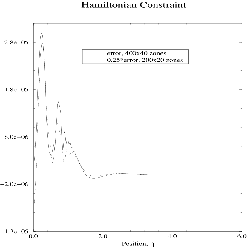
FIG. 1.: Numerical violation of the Hamiltonian constraint for the implosion of a dust shell onto a rotating black hole with $J=10$, as measured along $\theta=\pi/4$. We plot the constraint violation at high resolution and 1/4 the constraint violation at medium resolution. For second order convergence these curves should lie on top of one another.

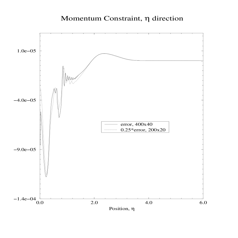
FIG. 2.: Numerical violation of the $\eta$-component of the momentum constraint for the implosion of a dust shell onto a rotating black hole with $J=10$, as measured along $\theta=\pi/4$. We plot the constraint violation at high resolution and 1/4 the constraint violation at medium resolution. For second order convergence these curves should lie on top of one another.

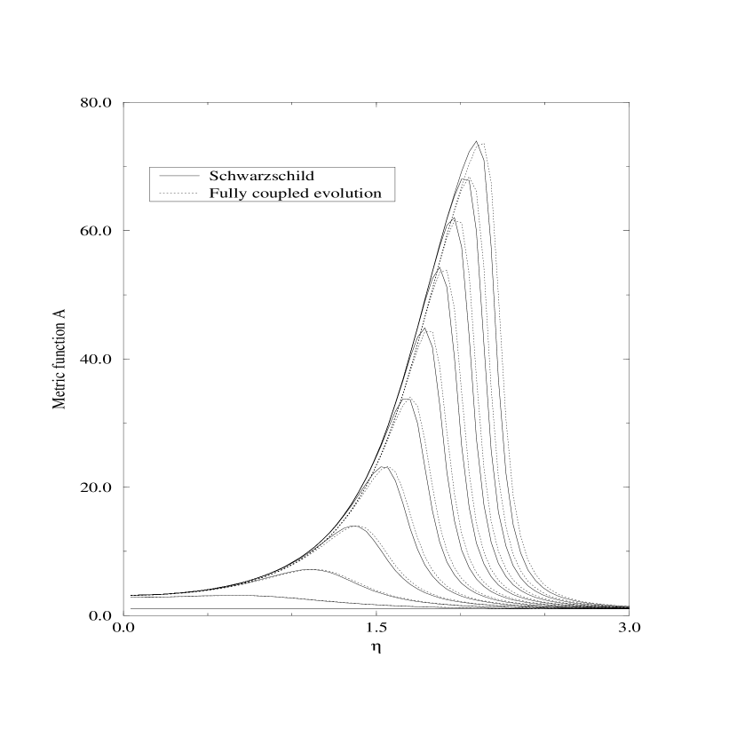
FIG. 4.: Time evolution of the metric component $A$ for two different couplings between the hydrodynamics and metric components of the code. The solid lines indicate Schwarzschild (i.e., matter flowing on a dynamically sliced background which cannot be affected by the matter fields) and the dotted lines correspond to a ful coupling (i.e., fully self-gravitating matter that is allowed to affect the spacetime geometry). The last curve corresponds to $t=50M_{ADM}$. The initial matter density is $\hat{\rho}=10^{-2}$. Almost no differences are found between the two evolutions for such low density matter flows.

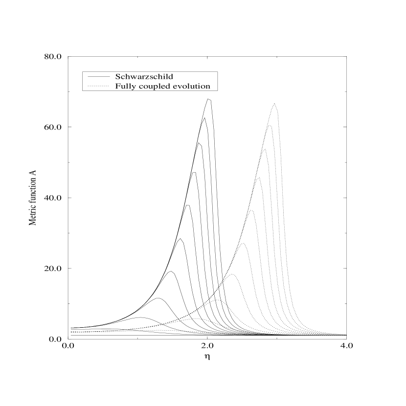
FIG. 5.: Same as Fig. 4 but for an initial uniform density distribution $\hat{\rho}=1$. Now, the evolution of the spacetime is noticeably different if the metric reacts or not to the presence of the matter.

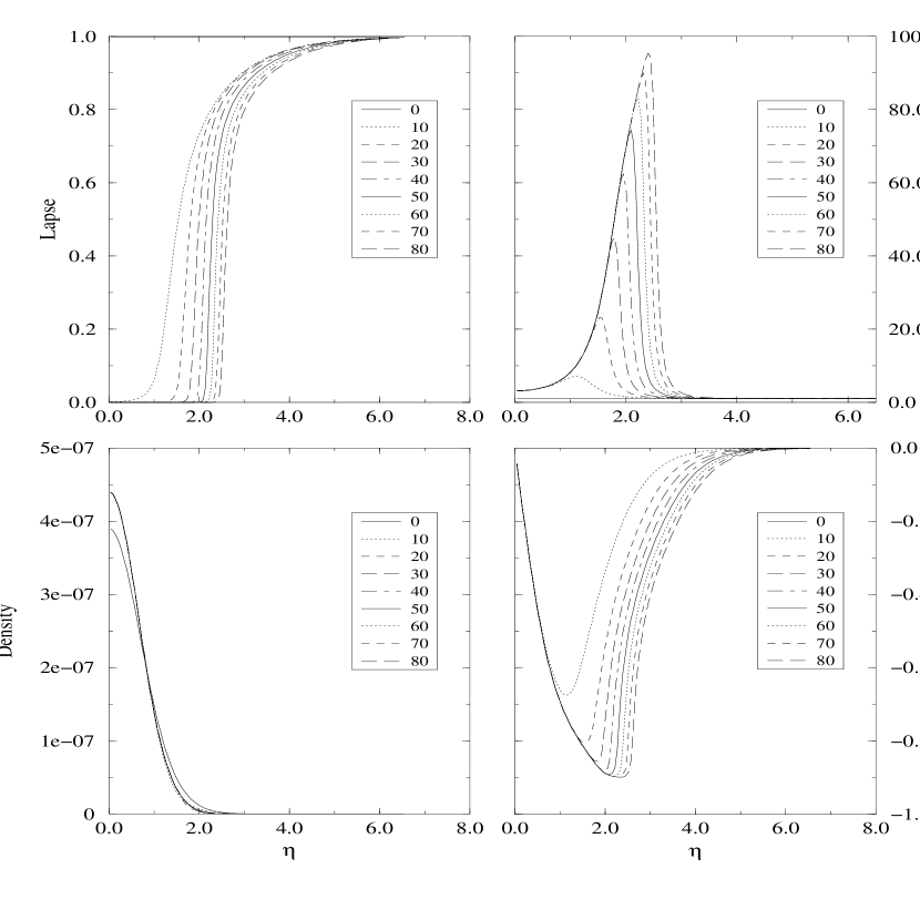
FIG. 6.: Evolution of different metric and hydrodynamical quantities for the problem of spherical accretion of dust with $\hat{\rho}=10^{-2}$. The top panels show the lapse (left) and the metric component labelled $A$. The bottom plots show the rest-mass density (left) and the total velocity of the dust particles.

FIG. 8.: Apparent horizon location as a function of time for the spherical dust accretion problem.

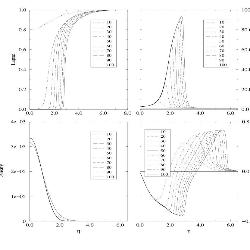
FIG. 9.: Evolution of different metric and hydrodynamical quantities for the problem of spherical accretion of a perfect fluid. The top panels show the lapse (left) and the metric component labelled $A$. The bottom plots show the rest-mass density (left) and the total velocity of the fluid.

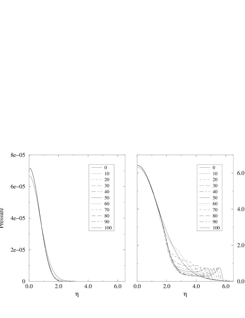
FIG. 10.: Evolution of the pressure (left) and internal energy density for the problem of spherical accretion of a perfect fluid with $\gamma=4/3$.

FIG. 11.: Different metric and hydrodynamic quantities for the impact of an imploding shell of dust with the black hole. The solution is plotted at a final time of $100M$. From top-left to bottom-right we show the density, total velocity, lapse and metric function $A$.

FIG. 12.: Radial profiles of the density at different times of the evolution of an imploding shell. They correspond to an arbitrary constant value of the angular coordinate. Notice the collapse of the shell in progressive times. The thick solid line shows the initial profile.

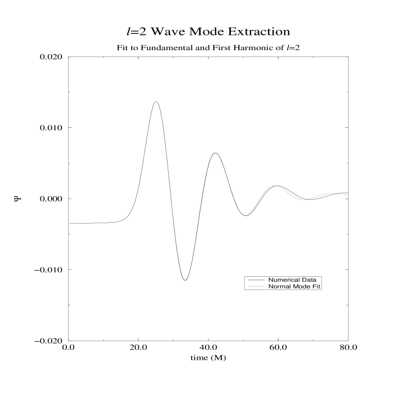
FIG. 13.: This figure shows the numerically extracted $\ell=2$ waveform (solid line) and the least squares fit to the two lowest $\ell=2$ quasinormal mode for the imploding shell problem.

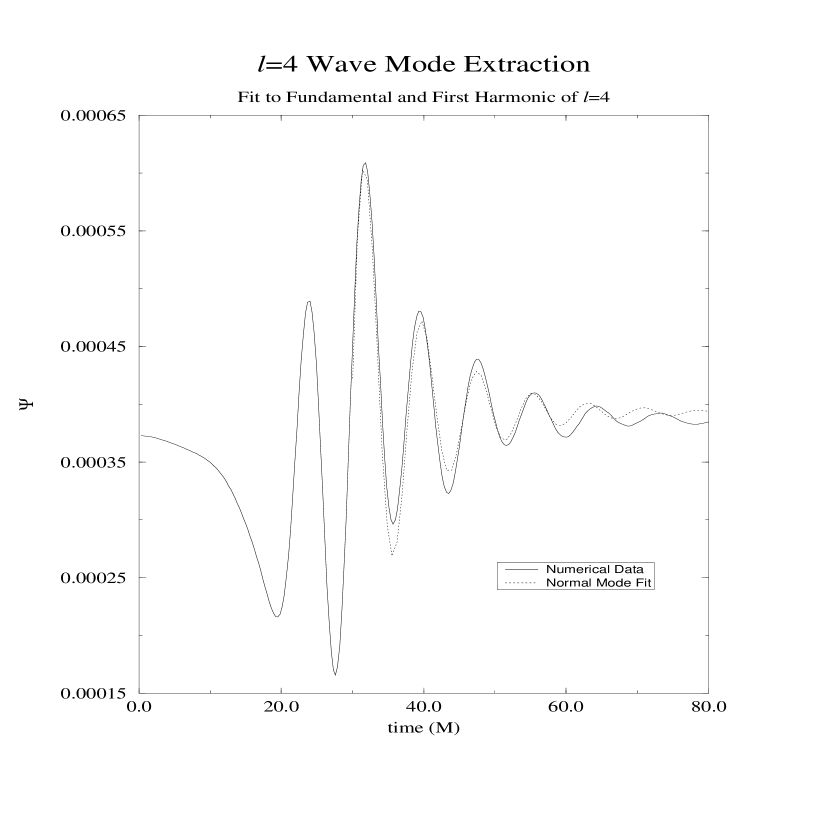
FIG. 14.: This figure shows the numerically extracted $\ell=4$ waveform (solid line) and the least squares fit to the two lowest $\ell=4$ quasinormal mode for the imploding shell problem.

FIG. 15.: This figure shows the energy accounting for a simulation with a Brill wave and matter fields at a variety of resolutions. The Brill wave amplitude is $0.5$, its width is $1.0$ and its location is $\eta_{0}=2.5$. The matter distribution is located at $\eta_{0}=2.0$ and has an amplitude of $3.0$. The background conformal density is $10^{-4}$.

FIG. 16.: Metric component $A$ at $t=25M_{ADM}$ for a rotating black hole spacetime with $J=20$. Notice the slightly less grid stretching near the equator as a consequence of the rotation.

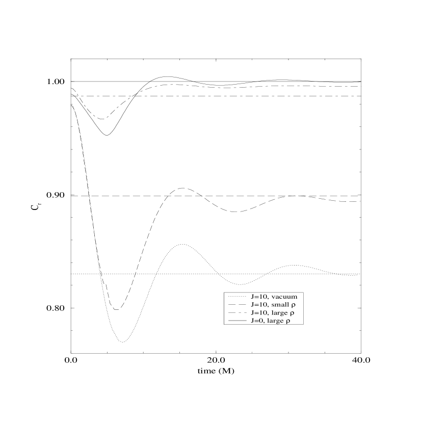
FIG. 17.: The ratio of the polar to equatorial circumference of the apparent horizon for a sample of rotating spacetimes. In each case, a horizontal line corresponding to the ratio for a Kerr black hole with the same ADM mass and angular momentum. The dotted line corresponds to a vacuum spacetime while the remaining three curves correspond to matter evolutions. One can easily see that only in the vacuum spacetime does the horizon settle down to something with the same shape as the Kerr black hole.

FIG. 18.: This figure shows the numerically extracted $\ell=2$ waveform (solid line) and the least squares fit to the two lowest $\ell=2$ quasinormal mode for the problem of the implosion of a dust shell onto a rotating black hole.

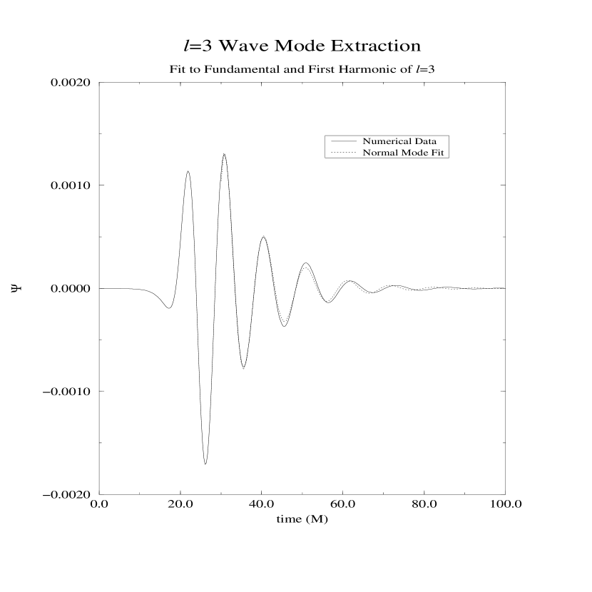
FIG. 19.: This figure shows the numerically extracted $\ell=2$ waveform (solid line) and the least squares fit to the two lowest $\ell=3$ quasinormal mode for the problem of the implosion of a dust shell onto a rotating black hole.

FIG. 20.: This figure shows the numerically extracted $\ell=2$ waveform (solid line) and the least squares fit to the two lowest $\ell=5$ quasinormal mode for the problem of the implosion of a dust shell onto a rotating black hole.

REFERENCES

- [1] M. M. May and R. H. White, Phys. Rev. D 141, 1232 (1966).
- [2] P. G. Dykema, Ph.D. thesis, University of Texas at Austin, 1980.
- [3] S. L. Shapiro and S. A. Teukolsky, ApJ 235, 199 (1980).
- [4] C. R. Evans, Ph.D. thesis, University of Texas at Austin, 1984.
- [5] P. J. Schinder, S. A. Bludmann, and T. Piran, Phys. Rev. D 37, 2722 (1988).
- [6] A. Mezzacappa and R. A. Matzner, ApJ 343, 853 (1989).
- [7] E. Gourgoulhon, Astron. Astroph. 252, 651 (1991).
- [8] J. V. Romero, J. M. Ibánez, J. M. Martí, and J. A. Miralles, ApJ 462, 839 (1996).
- [9] J. Hawley, L. Smarr, and J. Wilson, Astrophys. J. Suppl. Ser. 55, 211 (1984).
- [10] J. Hawley, L. Smarr, and J. Wilson, Astrophys. J. 277, 296 (1984).
- [11] L. I. Petrich, S. L. Shapiro, R. F. Stark, and S. A. Teukolsky, Astrophys. J. 336, 313 (1989).
- [12] F. Banyuls, J. A. Font, J. M. Ibánez, J. M. Martí, and J. A. Miralles, ApJ 476, 221 (1997).
- [13] J. A. Font and J. M. Ibánez, ApJ 494, 297 (1998).
- [14] T. Nakamura, Prog. Theor. Phys. 65, 1876 (1981).
- [15] R. F. Stark and T. Piran, Phys. Rev. Lett. 55, 891 (1985).
- [16] C. Evans, in Dynamical Spacetimes and Numerical Relativity, edited by J. Centrella (Cambridge University Press, Cambridge, England, 1986), pp. 3–39.
- [17] A. M. Abrahams, G. B. Cook, S. L. Shapiro, and S. A. Teukolsky, Phys. Rev. D 49, 5153 (1994).
- [18] J. Hawley, Astrophys. J. 381, 496 (1991).
- [19] C. Duncan, L. Sczaniecki, and G. Shastri, , preprint.
- [20] K.-I. Oohara and T. Nakamura, in Relativistic Gravitation and Gravitational Radiation, edited by J.-P. Lasota and J.-A. Marck (Cambridge University Press, Cambridge, England, 1997).
- [21] J. R. Wilson and G. J. Mathews, Phys. Rev. Lett. 75, 4161 (1995).
- [22] J. R. Wilson, G. J. Mathews, and P. Marronetti, Phys. Rev. D 54, 1317 (1996).
- [23] J. R. Wilson, ApJ 173, 431 (1972).
- [24] J. R. Wilson, in Sources of Gravitational Radiation, edited by L. Smarr (Cambridge University Press, Cambridge, England, 1979), p. 275.
- [25] A. Abrahams and C. Evans, Phys. Rev. D 46, R4117 (1992).
- [26] A. Abrahams and C. Evans, Phys. Rev. Lett. 70, 2980 (1993).
- [27] D. Bernstein, D. Hobill, E. Seidel, L. Smarr, and J. Towns, Phys. Rev. D 50, 5000 (1994).
- [28] D. Bernstein, D. Hobill, E. Seidel, and L. Smarr, Phys. Rev. D 50, 3760 (1994).
- [29] P. Anninos, D. Hobill, E. Seidel, L. Smarr, and W.-M. Suen, Phys. Rev. Lett. 71, 2851 (1993).
- [30] P. Anninos, D. Hobill, E. Seidel, L. Smarr, and W.-M. Suen, Phys. Rev. D 52, 2044 (1995).
- [31] S. Brandt and E. Seidel, Phys. Rev. D 52, 856 (1995).
- [32] S. Brandt and E. Seidel, Phys. Rev. D 52, 870 (1995).
- [33] P. Anninos, K. Camarda, J. Massó, E. Seidel, W.-M. Suen, and J. Towns, Phys. Rev. D 52, 2059 (1995).
- [34] P. Anninos, J. Massó, E. Seidel, W.-M. Suen, and M. Tobias, Phys. Rev. D 56, 842 (1997).
- [35] C. Bona, J. Massó, E. Seidel, and P. Walker, (1998), gr-qc/9804065. Submitted to Physical Review D.
- [36] J. M. Martí, J. M. Ibánez, and J. A. Miralles, Phys. Rev. D 43, 3794 (1991).
- [37] J. A. Font and J. M. Ibánez, MNRAS (1998), in press.
- [38] J. A. Font and J. Massó, Proceedings of the 8th Marcel Grossmann Meeting on General Relativity (World Scientific, Singapore, 1997).
- [39] M. A. Aloy, C. Bona, J. A. Font, J. M. Ibánez, J. Massó, and E. Seidel, (1998), in preparation.
- [40] C. Bona, J. Massó, E. Seidel, and J. Stela, Phys. Rev. Lett. 75, 600 (1995).
- [41] C. Bona, J. Massó, E. Seidel, and J. Stela, Phys. Rev. D 56, 3405 (1997).
- [42] J. A. Font, M. Miller, W. M. Suen, and M. Tobias, (1998), in preparation.
- [43] E. Bougleux and et al, (1998), in preparation.
- [44] S. Brandt and E. Seidel, Phys. Rev. D 54, 1403 (1996).
- [45] R. J. Leveque, Numerical Methods for Conservation Laws (Birkhauser Verlag, Basel, 1992).
- [46] S. K. Godunov, Mat. Sb. 47, 271 (1959), in Russian.
- [47] J. M. Martí, E. Müller, J. A. Font, J. M. Ibánez, and A. Marquina, ApJ 479, 151 (1997).
- [48] R. Arnowitt, S. Deser, and C. W. Misner, in Gravitation: An Introduction to Current Research, edited by L. Witten (John Wiley, New York, 1962), pp. 227–265.
- [49] J. York, in Sources of Gravitational Radiation, edited by L. Smarr (Cambridge University Press, Cambridge, England, 1979).
- [50] F. Estabrook, H. Wahlquist, S. Christensen, B. DeWitt, L. Smarr, and E. Tsiang, Phys. Rev. D 7, 2814 (1973).
- [51] D. Eardley and L. Smarr, Phys. Rev. D 19, 2239 (1979).
- [52] M. Duncan, Phys. Rev. D 31, 1267 (1985).
- [53] S. Schaffer, private communication.
- [54] L. Smarr and J. York, Phys. Rev. D 17, 1945 (1978).
- [55] N. O’Murchadha and J. York, Phys. Rev. D 10, 2345 (1974).
- [56] A. Lichnerowicz, J. Math Pures et Appl. 23, 37 (1944).
- [57] J. Bowen and J. W. York, Phys. Rev. D 21, 2047 (1980).
- [58] P. L. Roe, Journal of Computational Physics 43, 357 (1981).
- [59] R. Donat and A. Marquina, Journal of Computational Physics 125, 42 (1996).
- [60] R. Donat, J. A. Font, J. M. Ibánez, and A. Marquina, Journal of Computational Physics (1998), accepted.
- [61] C. W. Shu and S. J. Osher, Journal of Computational Physics 77, 439 (1988).
- [62] B. J. van Leer, Journal of Computational Physics 32, 101 (1979).
- [63] J. Font, J. Ibánez, J. Martí, and A. Marquina, Astron. Astrophys. 282, 304 (1994).
- [64] C. Bona, in Relativity and Scientific Computing, edited by F. Hehl (Springer-Verlag, Berlin, 1996).
- [65] O. Reula, Living Reviews in Relativity 1, (1998).
- [66] V. Moncrief, Annals of Physics 88, 323 (1974).
- [67] G. Allen, K. Camarda, and E. Seidel, (1998), gr-qc/9806014. Submitted to Phys. Rev. D.
- [68] K. Camarda and E. Seidel, , gr-qc/9805099. Submitted to Physical Review D.
- [69] P. Anninos, D. Bernstein, S. Brandt, J. Libson, J. Massó, E. Seidel, L. Smarr, W.-M. Suen, and P. Walker, Phys. Rev. Lett. 74, 630 (1995).
- [70] J. Libson, J. Massó, E. Seidel, W.-M. Suen, and P. Walker, Phys. Rev. D 53, 4335 (1996).
- [71] S. Hughes, C. R. K. II, P. Walker, K. Walsh, S. L. Shapiro, and S. A. Teukolsky, Phys. Rev. D 49, 4004 (1994).
- [72] J. Massó, E. Seidel, W.-M. Suen, and P. Walker, gr-qc/9804059. Submitted to Phys. Rev. D (1998).
- [73] J. York, in Frontiers in Numerical Relativity, edited by C. Evans, L. Finn, and D. Hobill (Cambridge University Press, Cambridge, England, 1989), pp. 89–109.
- [74] D. Christodoulou, Phys. Rev. Lett. 25, 1596 (1970).
- [75] H. Bondi, MNRAS 112, 195 (1952).
- [76] F. C. Michel, Astrophys. Spa. Sci. 15, 153 (1972).
- [77] T. Nakamura and M. Sasaki, Phys. Letters 106 B, 69 (1981).
- [78] S. L. Shapiro and I. Wasserman, ApJ 260, 838 (1982).
- [79] P. Papadapoulos and J. A. Font, (1998), in preparation.
- [80] S. A. Teukolsky, Astrophys. J. 185, 635 (1973).
- [81] L. L. Smarr, Phys. Rev. D 7, 289 (1973).
- [82] P. T. Leung, Y. T. Liu, , W.-M. Suen, C. Y. Tam, and K. Young, Physical Review Letters 78, 2894 (1997).