The projector on physical states in loop quantum gravity

Abstract

We construct the operator that projects on the physical states in loop quantum gravity. To this aim, we consider a diffeomorphism invariant functional integral over scalar functions. The construction defines a covariant, Feynman-like, spacetime formalism for quantum gravity and relates this theory to the spin foam models. We also discuss how expectation values of physical quantity can be computed.

I Introduction

The loop approach to quantum gravity [1] based on the Ashtekar variables [2] has been successful in establishing a consistent and physically reasonable framework for the mathematical description of quantum spacetime [3]. This framework has provided intriguing results on the quantum properties of space, most notably detailed quantitative results on the discrete quanta of the geometry [4]. The nonperturbative dynamics of the quantum gravitational field, however, is not yet well understood. Two major questions are open. First, several versions of the hamiltonian constraint have been proposed [5, 6, 7], but the physical correctness of these versions has been questioned [8]. Second, a general scheme for extracting physical consequences from a given hamiltonian constraint, and for computing expectations values of physical observables is not available.

In this paper, we address the second of these problems – a solution of which, we think, is likely to be a prerequisite for addressing the first problem (the choice of the correct hamiltonian constraint). The problem we address is how expectation values of physical observables can be computed, given a hamiltonian constraint operator $H(x)$. (For an earlier attempt in this direction, see [9].) We address this problem by constructing the “projector” $P$ on the physical Hilbert space of the theory, namely on the space of the solutions of the hamiltonian constraint equation. Formally, this projector can be written as

$$P\sim\prod_{x}\delta(H(x))\sim\int[DN]\ e^{-i\int d^{3}x\ N(x)H(x)}$$ (1)

in analogy with the representation of the delta function as the integral of an exponential. The idea treating first class constraints in the quantum theory by using a projector operator defined by a functional integration has been studied by Klauder [10], and consider also by Govaerts [11], Shabanov and Prokhorov [12], Henneaux and Teitelboim [13] and others. In the case of gravity, the matrix elements of $P$ between two states concentrated on two 3-geometries $g$ and $g^{\prime}$ can be loosely identified with Hawking’s propagator $P(g,g^{\prime})$, which is formally written in terms of a functional integral over 4-geometries [14].

A step towards the definition of the projector $P$ was taken in [6], where a perturbative expression for the exponential of the hamiltonian smeared with a constant function $N(x)=N$ was constructed. What was still missing was a suitable diffeomorphism invariant notion of functional integration over $N(x)$. Here, we consider an integration on the space of the scalar functions $N(x)$. This integral, modeled on the Ashtekar-Lewandowski construction [15] and considered by Thiemann in the context of the general covariant quantization of Higgs fields [16], allows us to give a meaning to the r.h.s. of (1). Using it, we succeed in expressing the (regularized) matrix elements of the projector $P$ in a well defined power expansion. We then give a preliminary discussion of the expectation values of physical observables. The construction works for a rather generic form of the hamiltonian constraint, which includes, as far a we know, the various hamiltonians proposed so far.

As realized in [6], the terms of the expansion of $P$ are naturally organized in terms of a four-dimensional Feynman-graph-like graphic representation. The expression (1) can thus be seen also as the starting point for a spacetime representation of quantum gravity. Here, we complete the translation of canonical loop quantum gravity into covariant spacetime form initiated in [6]. The “quantum gravity Feynman graphs” are two-dimensional colored branched surfaces, and the theory takes the form of a “spin foam model” in the sense of Baez [17], or a “worldsheet theory” in the sense of Reisenberger [18], or a “theory of surfaces” in the sense of Iwasaki [19], and turns out to be remarkably similar to the Barret-Crane model [20] and to the Reisenberger model [21] (see also [22]). On the one hand, the construction presented here provides a more solid physical grounding for these models; on the other hand, it allows us to reinterpret these models as proposals for the hamiltonian constraint in quantum gravity, thus connecting two of the most promising directions of investigations of quantum spacetime [23].

The paper is organized as follows. In Section II, the basics of loop quantum gravity are reviewed, organized from a novel and simpler perspective, which does not require the cumbersome introduction of generalized connections, or projective limits (see also [24]). Section III presents the definition of the diffeomorphism invariant functional integral. In section IV we construct the projector $P$ and discuss the construction of the expectation values.

II Loop quantum gravity

General relativity can be expressed in canonical form in term of a (real) $SU(2)$ connection $A$ defined over a 3d manifold $\Sigma$ [2, 25]. We take $\Sigma$ to be topologically $S_{3}$. The dynamics is specified by the usual Yang-Mills constraint, which generates local $SU(2)$ transformation, the diffeomorphism constraint $D[\vec{f}]$, which generates diffeomorphisms of $\Sigma$, and the Hamiltonian constraint $H[N]$, which generates the evolution of the initial data in the (physically unobservable) coordinate time. Here $\vec{f}$ is in the algebra of the group $Diff$ of the diffeomorphisms of $\Sigma$, namely it is a smooth vector field on $\Sigma$, and $N$ is a smooth scalar function on $\Sigma$. The theory admits a nonperturbative quantization as follows. (For a simple introduction, see [24], for details see [3] and references therein.)

A Hilbert space and spin networks basis

We start from the linear space $L$ of quantum states $\Psi(A)$ which are continuous (in the sup-topology) functions of (smooth) connections $A$. A dense (in $L$’s pointwise topology) subset of states in $L$ is formed by the graph-cylindrical states [15]. A graph-cylindrical state $\Psi_{\Gamma,f}(A)$ is a function of the connection of the form

$$\Psi_{\Gamma,f}(A)=f(U(e_{1},A),\ldots,U(e_{n}A)),$$ (2)

where $\Gamma$ is a graph embedded in $\Sigma$, $e_{1}\ldots e_{n}$ are the links of $\Gamma$, $U(e,A)={\cal P}exp\int_{e}A$ is the parallel propagator $SU(2)$ matrix of $A$ along the path $e$, and $f$ is a complex valued (Haar-integrable) function on $[SU(2)]^{n}$. The function $\Psi_{\Gamma,f}(A)$ has domain of dependence on the graph $\Gamma$; one can always replace $\Gamma$ with a larger graph $\Gamma^{\prime}$ such that $\Gamma$ is a subgraph of $\Gamma^{\prime}$, by simply taking $f$ independent from the group elements corresponding to the links in $\Gamma^{\prime}$ but not in $\Gamma$. Therefore any two given graph-cylindrical functions can always be viewed as defined on the same graph $\Gamma$. Using this, a scalar product is defined on any two cylindrical functions by

$$(\Psi_{\Gamma,f},\Psi_{\Gamma,g})=\int_{[SU(2)]^{n}}dU_{1}\ldots dU_{n}\ \overline{f(U_{1}\ldots U_{n})}\ g(U_{1}\ldots U_{n})$$ (3)

and extends by linearity and continuity to a well defined [15, 26] scalar product on $L$. The Hilbert completion of $L$ in this scalar product is the Hilbert space $H_{aux}$: the quantum state space on which quantum gravity is defined. We refer to [24] for the construction of the elementary quantum field operators on this space.

The $SU(2)$ gauge invariant states form a liner subspace $L_{0}$ in $L$. A convenient orthonormal basis in $L_{0}$ is the spin network basis [35], constructed as follow. Consider a graph $\Gamma$ embedded in $\Sigma$. To each link $e$ of $\Gamma$, assign a nontrivial $SU(2)$ irreducible representation $j_{e}$, which we denote the color of the link. Consider a node $n$ of $\Gamma$, where the links $e_{1}\ldots e_{N}$ meet; consider the invariant tensors $v$ on the tensor product of the representation $j_{e_{1}}\ldots j_{e_{N}}$ of the links that meet at the node; the space of these tensors is finite dimensional (or zero dimensional) and carries an invariant inner product. Choose an orthogonal basis in this space, and assign to each node $n$ of $\Gamma$ one element $v_{n}$ of this basis. A spin network $S=(\Gamma,\{j\},\{v\})$ is given by a graph $\Gamma$ and an assignment of a color $j_{e}$ to each link $e$ and a basis invariant tensor $v_{n}$ to each node $n$.

The spin network state $\Psi_{S}(A)$ is defined as

$$\Psi_{S}(A)=\prod_{e}\prod_{n}\ v_{n}\ R^{j_{e}}(U(e,A))$$ (4)

where $R^{j}(U)$ is the matrix representing the $SU(2)$ group element $U$ in the spin-$j$ irreducible representation, and the two matrix indices of $R^{j_{e}}(U(e,A))$ are contracted into the two tensors $v_{n}$ of the two nodes adjacent to $e$. An easy computation shows that (with an appropriate normalization of the basis states $v_{n}$ [27]) the states $\Psi_{S}$ form an orthonormal basis in $H_{aux}$

$$(\Psi_{S},\Psi_{S^{\prime}})=\delta_{\Gamma,\Gamma^{\prime}}\delta_{\{j\}\{j^{\prime}\}}\delta_{\{v\}\{v^{\prime}\}}.$$ (5)

B Diffeomorphisms

The Hilbert space $H_{aux}$ carries a natural unitary representation ${\cal U}(Diff)$ of the diffeomorphism group of $\Sigma$.

$$[{\cal U}(\phi)\psi](A)=\psi(\phi^{-1}A),\ \ \ \ \ \phi\in Diff.$$ (6)

It is precisely the fact that $H_{aux}$ carries this representation which makes it of crucial interest for quantum gravity. In other words, $H_{aux}$ and its elementary quantum operators represent a solution of the problem of constructing a representation of the semidirect product of a Poisson algebra of observables with the diffeomorphisms.[29]

Notice that ${\cal U}$ sends a state of the spin network basis into another basis state

$$[{\cal U}(\phi)\psi_{S}](A)=\psi_{S}(\phi^{-1}A)=\psi_{\phi S}(A).$$ (7)

Intuitively, the space $H_{diff}$ of the solutions of the quantum gravity diffeomorphism constraint is formed by the states invariant under ${\cal U}$. However, no finite norm state is invariant under ${\cal U}$, and generalized-state techniques are needed. We sketch here the construction of $H_{diff}$ [1, 26, 28], because the solution of the hamiltonian constraint will be given below along similar lines. $H_{diff}$ is defined first as a linear subset of $L^{*}$, the topological dual of $L$. It is then promoted to a Hilbert space by defining a suitable scalar product over it. $H_{diff}$ is the linear subset of $L^{*}$ formed by the linear functionals $\rho$ such that

$$\rho({\cal U}(\phi)\psi)=\rho(\psi)$$ (8)

for any $\phi\in Diff$. From now on we adopt a bra/ket notation. We write (8) as

$$\langle\rho|{\cal U}(\phi)\psi\rangle=\langle\rho|\psi\rangle$$ (9)

and we write the spin network state $\Psi_{S}$ as $|S\rangle$.

Equivalence classes of embedded spin networks under the action of Diff are denoted as $s$ and called s-knots, or simply spin networks. We denote as $s(S)$ the equivalence class to which $S$ belong. Every s-knot $s$ defines an element $\langle s|$ of $H_{diff}$ via

$$\langle s|S\rangle = 0,\ \ \ \rm{if}\ \ s\neq s(S)$$ (10)

$$= c_{s},\ \ \ \rm{if}\ \ s=s(S).$$ (11)

Here $c_{s}$ is the integer number of isomorphisms (including the identity) of the (abstract) colored graph of $s$ into itself that preserve the coloring and can be obtained from a diffeomorphism of $\Sigma$. A scalar product is then naturally defined in $H_{diff}$ by

$$\langle s|s^{\prime}\rangle\equiv\langle s|S^{\prime}\rangle$$ (12)

for an arbitrary $S^{\prime}$ such that $s(S^{\prime})=s^{\prime}$. One sees immediately that the normalized states $\frac{1}{\sqrt{c_{s}}}|s\rangle$ form an orthonormal basis.

The space $H_{diff}$ is not a subspace of $H_{aux}$ (because diff invariant states have “infinite norm”). Nevertheless, an important observation is that there is a natural “projector” $\Pi$ from $H_{aux}$ to $H_{diff}$

$$\Pi:|S\rangle\longmapsto|s(S)\rangle$$ (13)

which sends the state in $H_{aux}$ associated to an embedded spin network $S$ into the state in $H_{diff}$ associated to the corresponding abstract spin network state $s$. Notice that $\Pi$ is not really a projector, since $H_{diff}$ is not a subspace of $H_{aux}$, but we use the expression “projector” nevertheless, because of its physical transparency. Since $H_{diff}$ can be seen as a subspace of $H_{aux}^{*}$, the operator $\Pi$ defines a (degenerate) quadratic form $\langle\ |\ \rangle_{diff}$ on $H_{aux}$

$$\langle S|S^{\prime}\rangle_{diff}\equiv\langle S|\Pi|S^{\prime}\rangle=\langle s(S)|S^{\prime}\rangle=\langle s(S)|s(S^{\prime})\rangle.$$ (14)

$H_{diff}$ is can be defined also by starting with the pre-Hilbert space $H_{aux}$ equipped with the degenerate a quadratic form $\langle\ |\ \rangle_{diff}$, and factoring and completing the in the Hilbert norm defined by $\langle\ |\ \rangle_{diff}$ .[30] That is, states in $H_{aux}$ are the (limits of sequences of) equivalence classes of states in $H_{aux}$ under $\langle\ |\ \rangle_{diff}$. In other words, knowing the “matrix elements”

$$\langle S|\Pi|S^{\prime}\rangle$$ (15)

of the projector $\Pi$ is equivalent to having solved the diffeomorphism constraint.

Furthermore, the above construction can be expressed also in terms of certain formal expressions, which are of particular interest because they can guide us in solving the hamiltonian constraint. Define a formal integration over the diffeomorphism group $Diff$ satisfying the two properties

$$\int_{Diff}D\phi=1,$$ (16)

and

$$\int_{Diff}D\phi\ \delta_{S,\phi S}=c_{s(S)}.$$ (17)

Then a diff invariant state $|s\rangle$ can be written as a “state in $H_{aux}$ integrated over the diffeomorphism group”. That is

$$|s(S)\rangle=\int_{Diff}D\phi\ |{\cal U}(\phi)S\rangle,$$ (18)

In fact, the equations (11) and (12) can be obtained from the equations (16), (17) and (18). Using this, we can write the projection operator $\Pi$, defined in (13), as

$$\Pi=\int_{Diff}D\phi\ {\cal U}[\phi].$$ (19)

Equivalently, we may write the group element as an exponential of an algebra element, and formally integrate over the algebra rather than over the group, that is

$$\Pi=\int D\vec{f}\ e^{-iD[\vec{f}]}.$$ (20)

This equation has a compelling interpretation as the definition of the projector on the kernel of the diffeomorphism constraint operator $D_{a}(x)$ via

$$\Pi\sim\prod_{a,x}\ \delta(D_{a}(x))\sim\int D\vec{f}\ e^{-i\int d^{3}x\ f^{a}(x)D_{a}(x)}$$ (21)

as in

$$\delta(x)=\frac{1}{2\pi}\int_{-\infty}^{+\infty}dp\ e^{-ipx}.$$ (22)

We shall define the projector on the kernel of the hamiltonian constraint in a similar manner.

III A diffeomorphism invariant measure

In this section, we construct a measure on the space of scalar functions [16], which will be needed for defining the analog of Eq. 20 for the hamiltonian constraint. Consider smooth functions $N:\Sigma\rightarrow S_{1}$ on the three-manifold $\Sigma$, taking value on the interval $I=[0,T[$. We keep track of the “length of the interval $I$”, $T$, instead of normalizing it to one, because this will simplify keeping track of dimensions in the physical application. Let $\cal N$ be the space of such functions, equipped with the $sup$ topology. Let $F(N)$ be a continuous complex function on the infinite dimensional topological vector space $\cal N$, and denote the space of these functions as $\cal L$. Let $\{x_{i}\}=x_{1},\ldots,x_{n}$ be a set of (disjoint) points in $\Sigma$, and $f:(I)^{n}\rightarrow C$ a complex integrable function of $n$ real variables. Consider a function $F\in{\cal L}$ of the form

$$F_{\{x_{i}\},f}(N)=f(N(x_{1}),\ldots,N(x_{n})),$$ (23)

namely a function of $N$ having the the set $\{x_{i}\}$ as its domain of dependence. The set of functions of this form form a dense linear subspace of $\cal L$, in the pointwise topology.

The simplest nontrivial of such functions is obtained by picking a single point $x$ and choosing $f(N)=N$. Notice that this defines precisely the Gel’fand transform $F_{x}(N)=N(x)$, or in Gel’fand’s enchanting notation

$$x(N)=N(x).$$ (24)

Since the functions of the form (23) can be seen as a generalization of Gel’fand’s $F_{x}(N)$, we denote them as “generalized Gel’fand functions”, or simply Gel’fand functions. Gel’fand functions can be seen as the scalar-field analog of the Ashtekar-Lewandowski’s graph-cylindrical functions (2), which are defined for connection-fields.

Define the following linear form on the Gel’fand functions

$$\int DN\ F_{\{x_{i}\},f}(N)=\frac{1}{(T)^{n}}\int_{I^{n}}dN_{1}\ldots dN_{n}\ f(N_{1},\ldots,N_{n}).$$ (25)

Here $\frac{dN_{i}}{T}$ is the normalized invariant measure on the interval $I$. Finally, denote the closure of $\cal L$ in the norm

$$||F||=\int DN\ |F(N)|$$ (26)

as $L_{1}[{\cal N}]$; the linear form (25) extends by continuity (in the $L^{1}$ topology defined by this norm) to all of $L_{1}[{\cal N}]$.

A simple class of integrable functions is given by polynomial Gel’fand functions. We have indeed

$$\int DN\ 1 = \frac{1}{T}\int_{I}dN\ 1=1,$$ (27)

$$\int DN\ N(x) = \frac{1}{T}\int_{I}dN\ N=\frac{1}{T}\frac{1}{2}T^{2}=\frac{1}{2}T$$ (28)

Notice that for quadratic functionals we must distinguish two cases

$$\int DN\ N(x)\ N(y) = \frac{1}{T^{2}}\int_{I}\int_{I}dN_{1}dN_{2}\ N_{1}\ N_{2}=\frac{1}{4}\,T^{2},$$ (29)

$$\int DN\ N(x)\ N(x) = \frac{1}{T}\int_{I}dN\ N^{2}=\frac{1}{T}\ \frac{1}{3}\,T^{3}=\frac{1}{3}\,T^{2}.$$ (30)

Namely, we must distinguish the case in which the arguments of the two functions $N(\ )$ are distinct or the same. The general pattern should be clear. A general polynomial functional $F_{n_{1}\ldots n_{K}}$ will have $n_{k}$ points $x_{1}^{(k)}\ldots x_{n_{k}}^{(k)}$ in its domain of dependence in which the function $N(x)$ appear with power $k$. A simple calculation yields then

$$I_{n_{1}\ldots n_{K}} = \int DN\ F_{n_{1}\ldots n_{K}}$$ (31)

$$= \int DN\ [N(x_{1}^{(1)})\ldots N(x_{n_{1}}^{(1)})][N(x_{1}^{(2)})\ldots N(x^{(2)}_{n_{2}})]^{2}\ldots[N(x^{(K)}_{1})\ldots N(x^{(K)}_{n_{K}})]^{K}$$ (32)

$$= T^{\sum_{k}n_{k}}\ \prod_{k=1}^{K}\left(\frac{1}{k+1}\right)^{n_{k}}$$ (33)

$$\equiv d_{n_{1}\ldots n_{K}}$$ (34)

The diffeomorphism group $Diff$ of $\Sigma$ acts naturally on $\cal N$, via $(\phi N)(x)=N(\phi^{-1}(x))$, where $\phi:\Sigma\rightarrow\Sigma$ is in $Diff$. It is easy to see that the integral (25) is diffeomorphism invariant

$$\int[DN]\ F[\phi N]=\int[DN]\ F[N].$$ (35)

This follows from the fact that the r.h.s. of (25) is clearly insensitive to a diffeomorphism transformation on $N$.

IV Dynamics: the regularized propagator

We now come to the construction of the physical state space $H_{phys}$ and the partition function of the theory. We have to solve the Dirac’s hamiltonian constraint equation

$$H[N]\psi=0$$ (36)

for the quantum Hamiltonian constraint $H[N]$.

A The Hamiltonian constraint: first version

The operator $H[N]$ that we consider is a small modification of the Riemanian hamiltonian constraint defined in [5]. However, we make only use of the general structure of this operator, which is common to several of the proposed variants. We take a symmetric version of $H[N]$, which “creates” as well as “destroying” links. The matrix elements of $H[N]$ are given by

$$\langle\psi|H[N]|\phi\rangle\ =\ \langle\psi|C[N]|\phi\rangle\ +\ \overline{\langle\phi|C[N]|\psi\rangle}$$ (37)

where $C[N]$ is the non-symmetric Thiemann’s constraint.

We recall that the operator $C[N]$, acting on a spin network state $|s\rangle$, is given by a sum of terms, one per each node $i$ of $s$. Sketchy (a more precise definition will be given below), each such term creates an extra link $e_{added}$ joining two points, $i^{\prime}$ and $i^{\prime}{}^{\prime}$, on two distinct links adjacent to $i$, and alters the colors of the links between $i$ and $i^{\prime}$ and between $i$ and $i^{\prime}{}^{\prime}$. The result is multiplied by a coefficient depending only on the colors of $s$, and by the value of the smearing function $N$ “in the point where the node $i$ is located”. This is illustrated in Figure 1.

FIG. 1.: Action of the hamiltonian constraint on a trivalent node.

It is important to observe that $C[N]$ is defined as a map from $H_{diff}$ to $H_{aux}^{*}$. In this definition there is a subtle interplay between diff-invariant and non-diff-invariant aspects of the hamiltonian constraint, which is a key aspect of the issue we are considering, and must be dealt with with care. The reason $C[N]$ is defined on $H_{diff}$, namely on the diffeomorphism invariant states, is that it is on these states that the “precise position” of the points $i$ and $i^{\prime}{}^{\prime}$ and of the link $e_{added}$ is irrelevant. However, $C[N]$ is not diffeomorphism invariant, and therefore $C[N]|s\rangle$ is not in $H_{diff}$, because a diffeomorphism modifies $N$. The feature of $C[N]|s\rangle$ that breaks diffeomorphism invariance is the fact that it contains a factor given by the value of $N(x)$ in the point in which the node $i$ is located: this location is not a diffeomorphism invariant notion.

Before presenting the precise definition of $C[N]$, which takes care both of its diff-invariant and its non-diff-invariant features, we need to define certain peculiar elements of $H_{aux}^{*}$, which will appear in the definition. Consider an s-knot $s$ and let $i$ be one of its nodes. Let $N$ be a scalar function on $\Sigma$. We define the state $|s;i,N\rangle$ in $H_{aux}^{*}$ by (again, we interchange freely bra and ket notation)

$$\langle s;i,N|S\rangle=N(x_{S,i})\ \langle s|S\rangle.$$ (38)

where $x_{S,i}$ is the position of the node of $S$ that gets identified with the node $i$ of $s$ in the scalar product. Notice that the state $|s;i,N\rangle$ is “almost” a diff-invariant s-knot state: in facts, it is “almost” insensible to the location of $S$. The only aspect of this location to which it is sensible is the location of the node. In fact, in the r.h.s. of (38), the diff invariant quantity $\langle s|S\rangle$ is multiplied by the value of $N(\ )$ in the point in which the node $i$ is located. The Hamiltonian constraint defined by Thiemann acts on diff-invariant states and creates states in $H_{aux}^{*}$, of the form (38).

The precise definition of $C[N]$ is the following

$$C[N]|s\rangle=A_{i}^{\beta}(s)\ |s_{i}^{\beta};i,N\rangle.$$ (39)

Let us explain our notation. Sum over the repeated indices $\beta$ and $i$ is understood. The index $i$ runs over the nodes in $s$. The index $\beta=(l^{\prime},l^{\prime}{}^{\prime},\epsilon^{\prime},\epsilon^{\prime}{}^{\prime})$ runs over the couples $(l^{\prime},l^{\prime}{}^{\prime})$ of (distinct) links adjacent to each node $i$ and over $\epsilon^{\prime}$ and $\epsilon^{\prime}{}^{\prime}$, which take the values $+1$ or $-1$. The s-knot $s_{i}^{\beta}$ was introduced in [32]. It is defined as the right hand part of Figure 1. That is, by adding two new nodes $i^{\prime}$ and $i^{\prime}{}^{\prime}$ on the two links $l^{\prime}$ and $l^{\prime}{}^{\prime}$ (determined by $\beta$) respectively, adding a new link $e_{added}$ colored $1/2$ joining $i^{\prime}$ and $i^{\prime}{}^{\prime}$, and altering the color of the links joining $i^{\prime}$ and $i$ (and, respectively, $i^{\prime}{}^{\prime}$ and $i$) by $+1$ or $-1$ according to the value of $\epsilon^{\prime}$ (respectively $\epsilon^{\prime}{}^{\prime}$). $A_{i}^{\beta}(s)$ is a coefficient defined in [5] whose explicit form is computed in [31].

Summarizing, we have

$$\langle S|C[N]|s\rangle=A_{i}^{\beta}(s)\ N(x_{S,i})\ \langle S|s_{i}^{\beta}\rangle.$$ (40)

(where $\langle S|s\rangle\equiv\langle s|S\rangle=\langle s|s(S)\rangle$; see (11) and (14).) Clearly, $C[N]$ can equivalently be viewed as an operator from $H_{aux}$ to $H_{diff}^{*}$, by writing

$$\langle s|C[N]|S\rangle=A_{i}^{\beta}(s)\ N(x_{S,i})\ \langle s|s(S)_{i}^{\beta}\rangle.$$ (41)

(Recall that $s(S)$ is the s-knot to which $S$ belongs.) This fact allows us to define the symmetrized operator (37) by

$$\langle S|H[N]|s\rangle=A_{i}^{\beta}(s)\ N(x_{S,i})\ \langle S|s_{i}^{\beta}\rangle+\overline{A}_{i}^{\beta}(s)\ N(x_{S,i})\ \langle s(S)_{i}^{\beta}|s\rangle.$$ (42)

Only one of the two terms in the r.h.s. of this equation may be non-vanishing: the first, if $S$ has two nodes more than $s$; the second, if $S$ has two nodes less than $s$.

We can simplify our notation by introducing an index $\alpha=(\beta,\pm 1)$ where $+1$ indicates that a link is added and $-1$ indicates that the link is removed. We obtain

$$\langle S|H[N]|s\rangle=A_{i}^{\alpha}(s)\ N(x_{S,i})\ \langle S|s_{i}^{\alpha}\rangle$$ (43)

where

$$A_{i}^{\beta,-1}(s)=\overline{A}_{i}^{\beta,+1}(s_{i}^{\beta}).$$ (44)

Notice that the precise position of $e_{added}$ (and thus $i^{\prime}$ and $i^{\prime}{}^{\prime}$) drops out from the final formula, because of the diff invariance of the quantity $\langle S|s_{i}^{\alpha}\rangle$. This is essential, because if a specific position for $e_{added}$ had to be chosen, diffeomorphism¡¡¡¡¡¡w invariance would be badly broken. One can view the coordinate distance $\epsilon$ between $i$ and $i^{\prime}$ (and between $i$ and $i^{\prime}{}^{\prime}$) as a regulating parameter to be taken to zero after the matrix elements (41) have been evaluated. The limit $\epsilon\to 0$ is discontinuous, but $\langle s|S_{i}^{\beta}\rangle$ is independent from $\epsilon$ for $\epsilon$ sufficiently small, and therefore the limit of these matrix elements is trivial. Thus, the operator is defined thanks to two key tricks:

1. the diff invariance of the state $|s\rangle$ acted upon allows us to get rid of the precise position of $e_{added}$;

2. the lack of diff invariance of $\langle S|$, allows us to give meaning to the point $x_{S,i}$ “where the node is located”, and therefore allows us to give meaning to the smearing of the operator with a given (non diff invariant!) function $N(x)$.

This is why $H[N]$ is defined as a map from $H_{diff}$ to $H_{aux}^{*}$. The first of these two key facts, which allow the quantum hamiltonian constraint operator to exist, was recognized in [32], the second in [5].

B The Hamiltonian constraint: second version

The interplay between diff invariant and non diff invariant constructs described above needs to be crafted even more finely, in order to be able to exponentiate the Hamiltonian constraint and derive its kernel. In fact, in order to exponentiate $H[N]$ and to expand the exponential in powers, we will have to deal with products of $H[N]$’s. In order for these products to be well defined, the domain of the operator must include its range, which is (essentially) $H_{aux}$. Therefore we need to extend the action of $H[N]$ from $H_{diff}$ to $H_{aux}$. The price for this extension is, of course, that the operator becomes dependent on the regulator, namely on the precise position in which $e_{added}$ is added. However, we can do so here, because such dependence will disappear in the integration over $N$ !

We define $H[N]$ on $H_{aux}$ by simply picking a particular position for $e_{added}$ in the definition of $S_{i}^{\alpha}$

$$H[N]|S\rangle=N(x_{i})\ A_{i}^{\alpha}(S)\ |S_{i}^{\alpha}\rangle.$$ (45)

where, clearly, $A_{i}^{\alpha}(S)=A_{i}^{\alpha}(s(S))$. (When $\alpha=(\beta,-1)$, no modification is necessary. That is, a link is removed irrespectively from its precise location.) In a quadratic expression this yields

$$\langle S|H[N]H[N]|s\rangle=A_{i}^{\alpha}(S_{i_{1}}^{\alpha_{1}})\ A_{i}^{\alpha}(S)\ N(x_{S{}_{i_{1}}^{\alpha_{1}}{}_{i_{2}}^{\alpha_{2}},i_{2}})\ N(x_{S_{i_{1}}^{\alpha_{1}},i_{1}})\ \langle S|s{}_{i_{1}}^{\alpha_{1}}{}_{i_{2}}^{\alpha_{2}}\rangle.$$ (46)

Here $i_{1}$ labels the nodes of $s$. After the action of the first operator, and thus the addition (or subtraction) of one link, we obtain $s_{i_{1}}^{\alpha_{1}}$. The index $i_{2}$ runs over the nodes of $s_{i_{1}}^{\alpha_{1}}$, and therefore its range is larger (or smaller) than the index $i_{1}$, because of the two new nodes (or the two nodes removed).

Notice that in each of the terms of the sum in the r.h.s. of (46) (that is, for each fixed value of the indices $i_{1},\alpha_{1},i_{2},\alpha_{2}$) we have a product

$$N(y)\ N(x)$$ (47)

where $x$ and $y$ are the positions of the two nodes acted upon by the two operators. In particular, the second $H[N]$ operator may act on one of the nodes created by the first operator $H[N]$. For instance, $x$ in (47) may be the coordinates of the point $i$ in (the l.h.s. of) Figure (1), and $y$ may be the coordinates of the point $i^{\prime}$ (in the r.h.s. of the Figure). Now, later on, expressions such as (46) will appear within functional integrals over $N$. Inside these integrals, the only feature of these two positions that matter is whether $x=y$ or not (see section III). Therefore, the only feature of the position of $e_{added}$ that matters is whether its end points, namely $i^{\prime}$ and $i^{\prime}{}^{\prime}$ in Figure 1, are on top of $i$ or not. This is the only dependence on the regulator (the position of $e_{added}$) that survives in the integral ! More precisely, in the integration over $N$, the arbitrariness in the regularization reduced to the arbitrariness of the decision of whether or not we should think at $i$, $i^{\prime}$ and $i^{\prime}{}^{\prime}$ in the r.h.s. of Figure 1, as on top of the point $i$ on the l.h.s. or not.

We can view this choice in the following terms. The operator $C[N]$ creates new nodes at positions which are displaced from the original node by a distance $\epsilon$, where $\epsilon$ is to be later taken to zero (taking this limit is in fact necessary in order to identify the quantum operator with the desired classical quantity). The choice is whether to take $\epsilon$ to zero before or after the integration over $N$.

Let us denote the position of the node $i$ of $S$ (the node acted upon) by $x$. Denote the two new nodes created by the action of the operator as $y^{\prime}$ and $y^{\prime}{}^{\prime}$. And denote the position of the node $i$ after the action of the operator as $y$ (nothing forces $x=y$ a priori). The natural choices are

1. $y=x$, $y^{\prime}\neq x$, $y^{\prime}{}^{\prime}\neq x$,

2. $y\neq x$, $y^{\prime}\neq x$, $y^{\prime}{}^{\prime}\neq x$,

3. $y=x$, $y^{\prime}=x$, $y^{\prime}{}^{\prime}=x$.

The choice is exquisitely quantum field theoretical: we are defining here the product of operator valued distributions, and we encounter an ambiguity in the renormalization of the regularized product. We thus have three options for the regularization of the operator products $C[N]\ldots C[N]$, corresponding to the three choices above.

Choice 3 is not (easily) compatible with the symmetrization of the operator, and choice 2 yields a nonsensical vanishing of all the matrix elements of the projector. Thus, we adopt, at least provisionally, choice 1 (which, after all, is probably the most natural). That is, we assume that $i$ itself is not displaced by the hamiltonian constraint operator, while $i^{\prime}$ and $i^{\prime}{}^{\prime}$ are created in positions which are distinct from the position of $i$ (see Figure 1).

For a product of $n$ operators (with the same smearing function), we have

$$\langle S|(H[N])^{n}|s\rangle=N(x_{1})\ldots N(x_{n})\ A_{i_{1}}^{\alpha_{1}}(S)\ldots A_{i_{n}}^{\alpha_{n}}(S_{i_{1}\ldots i_{n-1}}^{\alpha_{1}\ldots\alpha_{n-1}})\ \langle S|{s^{\prime}}_{i_{1}\ldots i_{n}}^{\alpha_{1}\ldots\alpha_{n}}\rangle,$$ (48)

where $i_{j}$ runs over the nodes of ${s^{\prime}}_{i_{1}\ldots i_{j-1}}^{\alpha_{1}\ldots\alpha_{j-1}}$, and we have denoted simply as $x_{1}\ldots x_{n}$ the positions of the sequence of nodes acted upon in a given term. According to the regularization chosen, this sequence contains points which are distinct except when a node is acted upon repeatedly.

C Expansion

Our task is now to define the space $H_{phys}$, using the various tools developed above. We aim at defining $H_{phys}$ following the lines $H_{diff}$ is defined by the operator $\Pi$ in equations (20) and (14). That is, we want to construct the operator

$$P=\int DN\ e^{-iH[N]},$$ (49)

whose matrix elements

$$\langle s|P|s^{\prime}\rangle=\int DN\ \langle s|e^{-iH[N]}|s^{\prime}\rangle.$$ (50)

define the quadratic form

$$\langle s|s^{\prime}\rangle_{phys}=\langle s|P|s^{\prime}\rangle.$$ (51)

$H_{phys}$ is then the Hilbert space defined over the pre-Hilbert space $H_{diff}$ by the quadratic form $\langle\ |\ \rangle_{phys}$. As for $\Pi$ (see section II B), we will call $P$ a “projector”, slightly forcing the usual mathematical meaning of this term.

Notice that the Hamiltonian constraint we use is a density of weight one (instead than two, as in the original Ashtekar formalism); therefore the integration variable $N$ is a scalar field. This fact will allow us to interpret the integration in $N$ in terms of the integral defined in section III. The importance of having a weight-one hamiltonian constraint in the quantum theory, was realized by Thiemann [5].

We begin by regularizing the integral (50) by restricting the integration domain of the functional integral in $[DN]$ to the subdomain formed by all the functions $N$ that satisfy

$$|N(x)|<T$$ (52)

where $T$ is a regularization parameter with the dimensions of a time. The physical limit is recovered for $T\to\infty$. We write

$$\langle s|P_{T}|s^{\prime}\rangle\equiv\int_{|N(x)|<T}DN\ \langle s|e^{-iH[N]}|s^{\prime}\rangle.$$ (53)

Notice that the regularization (52) is diffeomorphism invariant.

By taking advantage from the diff invariance of the expression (53), we can insert an integration over the diffeomorphisms and rewrite (53) using (18) as

$$\langle s|P_{T}|s^{\prime}\rangle=\int_{Diff}D\phi\int_{|N(x)|<T}DN\ \langle{\cal U}(\phi)S|e^{-iH[N]}|s^{\prime}\rangle$$ (54)

where $S$ is any spin network such that

$$s(S)=s.$$ (55)

Next, we expand the exponent in powers

$$\langle s|P_{T}|s^{\prime}\rangle=\int_{Diff}D\phi\int_{|N(x)|<T}DN\ \langle{\cal U}(\phi)S|\left(\sum_{n=0}^{\infty}\frac{(-i)^{n}}{n!}(H[N])^{n}\right)|s^{\prime}\rangle.$$ (56)

Using the explicit form (48) of the hamiltonian constraint operator and acting with ${\cal U}(\phi)$ explicitly we obtain

$$\langle s|P_{T}|s^{\prime}\rangle = \sum_{n=0}^{\infty}\frac{(-i)^{n}}{n!}\int_{Diff}D\phi\int_{|N(x)|<T}DN\ N(\phi(x_{i_{n}}))\ldots N(\phi(x_{i_{1}}))$$ (58)

$$\times A_{i_{n}}^{\alpha_{n}}(s_{i_{1}\ldots i_{n-1}}^{\alpha_{1}\ldots\alpha_{n-1}})\ldots A_{i_{1}}^{\alpha_{1}}(s)\ \langle s|{s^{\prime}}_{i_{1}\ldots i_{1}}^{\alpha_{1}\ldots\alpha_{n}}\rangle,$$

where $i_{j}$ runs over the nodes of ${s^{\prime}}_{i_{1}\ldots i_{j-1}}^{\alpha_{1}\ldots\alpha_{j-1}}$. We have also used (55) and

$$s(S_{i_{1}\ldots i_{j}}^{\alpha_{1}\ldots\alpha_{j}})=s_{i_{1}\ldots i_{j}}^{\alpha_{1}\ldots\alpha_{j}}.$$ (59)

which follows from it. Notice that, as promised, the only remaining diff-dependent quantities are the arguments of the functions $N(\ )$. But since the $DN$ integral is diff invariant (see Eq. (35)), the integration over $Diff$ can be trivially performed using (16). Also, notice that the $N(x)$’s appear only in the polynomials. Thus we have

$$\langle s|P_{T}|s^{\prime}\rangle=\sum_{n=0}^{\infty}\ \frac{(-i)^{n}}{n!}\ I_{x_{i_{n}}\ldots x_{i_{1}}}(T)\ \ A_{i_{n}}^{\alpha_{n}}(S_{i_{1}\ldots i_{n-1}}^{\alpha_{1}\ldots\alpha_{n-1}})\ldots A_{i_{1}}^{\alpha_{1}}(S)\ \langle s|{s^{\prime}}_{i_{1}\ldots i_{1}}^{\alpha_{1}\ldots\alpha_{n}}\rangle,$$ (60)

where

$$I_{x_{i_{n}}\ldots x_{i_{1}}}(T)=\int_{|N(x)|<T}DN\ N(x_{i_{n}})\ldots N(x_{i_{1}}).$$ (61)

Now, the last integral is precisely the integral of a polynomial Gel’fand function discussed in the previous section. The only difference here is that the domain of the $dN$ integral is between $-T$ and $T$ instead than between $0$ and $T$. The effect of this is just to put all the odd terms to zero and to double the even terms. Let $n_{k}$ be the number of points that appear $k$ times in the list $x_{i_{n}}\ldots x_{i_{1}}$, so that

$$\sum_{k}kn_{k}=n.$$ (62)

We obtain

$$I_{x_{i_{n}}\ldots x_{i_{1}}}(T)=\left(\prod_{k}e(k)\right)d_{n_{1}\ldots n_{k}}$$ (63)

where $d_{n_{1}\ldots n_{k}}$ is defined in Eq. (34), and $e(k)$ is defined for any integer $n$ by

$$e(2n) = 2,$$ (64)

$$e(2n+1) = 0.$$ (65)

From (34), and (62), we have

$$I_{x_{i_{n}}\ldots x_{i_{1}}}(T)=\prod_{k}e(k)\left(\frac{T^{k}}{k+1}\right)^{n_{k}}=T^{n}\prod_{k}\frac{e(k)}{(k+1)^{n_{k}}}$$ (66)

Inserting (66), in (60), we conclude

$$\langle s|P_{T}|s^{\prime}\rangle = \sum_{n=0}^{\infty}\ \ T^{n}\ \ \langle s|P^{(n)}|s^{\prime}\rangle$$ (67)

$$\langle s|P^{(n)}|s^{\prime}\rangle = \frac{(-i)^{n}}{n!}\sum_{i_{1}\ldots i_{n}\alpha_{1}\ldots\alpha_{n}}\prod_{k}\ \frac{e(k)}{(k+1)^{n_{k}}}\ \ A_{i_{n}}^{\alpha_{n}}(s_{i_{1}\ldots i_{n-1}}^{\alpha_{1}\ldots\alpha_{n-1}})\ldots A_{i_{1}}^{\alpha_{1}}(s)\ \langle s|{s^{\prime}}_{i_{1}\ldots i_{1}}^{\alpha_{1}\ldots\alpha_{n}}\rangle$$ (68)

We recall that the technique for the explicit computation of the coefficients $A_{i}^{\alpha}(s)$ is given in [31]. The last equation is an explicit and computable expression, term by term finite, for the regularized matrix elements of the projector on the physical state space of the solutions of the hamiltonian constraint.

D Interpretation: spin foam

The terms of the sum (68) are naturally labeled by branched colored surfaces [6, 17, 18], or “spin foams”. Each surface represents a history of the s-knot state. More precisely, consider a finite sequence $\sigma_{n}$ of $n+1$ spin networks

$$s_{0},s_{1}\ldots,s_{n}$$ (69)

In particular, let the sequence (69) be generated by a sequence of $n$ actions of single terms of the Hamiltonian constraint acting on $s_{0}$

$$\sigma_{n}=\left\{s,\ s_{i_{1}}^{\alpha_{1}},\ s_{i_{1}i_{2}}^{\alpha_{1}\alpha_{2}},\ \ldots,\ s_{i_{1}\ldots i_{n}}^{\alpha_{1}\ldots\alpha_{n}}\right\}$$ (70)

We call such a sequence a “spin foam”, and we represent it as a branched colored 2d surface. A branched colored surface is a collection of elementary surfaces (faces) carrying a color. The faces join in edges carrying an intertwiner. The edges, in turn, join in vertices. A branched colored surface with $n$ vertices can be identified with a sequence (70) if it can be sliced (in “constant time” slices) such that any slice that does not cut a vertex is one of the spin networks in (70). In other words, the branched colored surface can be seen as the spacetime world-sheet, or world-history of the spin network that evolves under $n$ actions of the hamiltonian constraint.

Each action of the hamiltonian constraint splits a node of the spin network into three nodes (or combine three nodes into one), and thus generates a vertex of the branched surface. Thus, as in the usual Feynman diagrams, the vertices describe the elementary interactions of the theory. In particular, here one sees that the complicated action of the hamiltonian displayed in Figure 1, which makes a node split into three nodes, corresponds to the simplest geometric vertex. Figure 2 is a picture of the elementary vertex. Notice that it represents nothing but the spacetime evolution of the elementary action of the hamiltonian constraint, given in Figure 1.

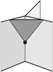
FIG. 2.: The elementary vertex.

An example of a surface in the sum is given in Figure 3.

FIG. 3.: A term of second order.

We write $\partial\sigma_{n}=s\cup s^{\prime}$ to indicate that the spin foam $\sigma_{n}$ is bounded by the initial and final spin networks $s$ and $s^{\prime}$. We associate to each $\sigma_{n}$ the amplitude

$$A(\sigma_{n})=\frac{1}{n!}\prod_{v=1}^{n}A(v)\prod_{k}\frac{e(k)}{(k+1)^{n_{k}}}$$ (71)

where $v$ run over the vertices of $\sigma_{n}$ and the amplitude of a single vertex is

$$A(v)=A_{i_{v}}^{\alpha_{v}}(s_{i_{1}\ldots i_{v-1}}^{\alpha_{1}\ldots\alpha_{v-1}}).$$ (72)

The amplitude of a vertex depends only on the coloring of the faces and edges adjacent to the vertex.

Using this, we can rewrite Eqs. (67, 68) as

$$\langle s|P_{T}|s^{\prime}\rangle=\sum_{n=0}^{\infty}\ \ T^{n}\sum_{\sigma_{n},\partial\sigma_{n}=s\cup s^{\prime}}A(\sigma_{n}).$$ (73)

The key novelty with respect to [6] is the factor

$$\prod_{k}\frac{e(k)}{(k+1)^{n_{k}}}$$ (74)

The integers $n_{k}$ are determined by the number of multiple actions of $H[N]$ on the same vertex.

The last expression leads immediately to the form of the (regularized) “vacuum to vacuum” transition amplitude, or the partition function of the theory

$$Z_{T}=\sum_{n=0}^{\infty}T^{n}\ \sum_{\sigma_{n}}A(\sigma_{n})$$ (75)

for $\sigma$’s with no boundaries. In words, the theory is defined as a sum over spin foams $sigma_{n}$, where the amplitude $A(\sigma_{n})$ of a spin foam is determined, via (71), by the product of the amplitudes $A(v)$ of its vertices. Thus, the theory is determined by giving the amplitude $A(v)$ of the vertex, as a function of adjacent colors.

E Physical observables

The expressions we have defined depend on the regulator $T$. A naive limit $T\to\infty$ yields to meaningless divergences. On the other hand, it is natural to expect to be able to remove the regulator only within expressions for physical expectation values. Loosely speaking, the integral (49) defines a delta-like distribution, and does not converge to any function itself; however, its contraction with a smooth function should converge. In particular, for finite $T$ the integral contracted with a function gives the integral of the Fourier transform of the function over the interval $[-T,T]$. If the function has a Fourier transform that decays reasonably fast, then the integral should converges nicely. Thus, we may expect the expansion in $T$ to be meaningful for suitable observables (see next section).

The difficulty of constructing interesting physical observables invariant under four-dimensional diffeomorphisms in general relativity in well known [33] and we do not discuss this problem here. Instead, we notice that given an operator $A$ on $H_{diff}$, invariant under three-dimensional diffeomorphisms, one can immediately construct a fully gauge invariant operator $O$ simply by

$$O=P\ A\ P.$$ (76)

For instance, $A$ may be the volume $V$ of $\Sigma$ operator [4, 34]; or the projector on a given eigenspace of $V$

$$A=\delta(V,v)$$ (77)

where $v$ is one of the eigenvalues of $V$. Consider the expectation value of $O$ in a physical state

$$\langle O\rangle=\frac{\langle s|O|s\rangle_{phys}}{\langle s|s\rangle_{phys}}=\frac{\langle s|PAP|s\rangle}{\langle s|P|s\rangle}.$$ (78)

While we expect this quantity to be finite (for an appropriate $A$), the numerator and the denominator are presumably independently divergent, as one may expect in a field theory. Our strategy to compute $\langle O\rangle$, therefore, must be to take the $T\to\infty$ limit of the ratio, and not of the numerator and of the denominator independently. We thus properly define

$$\langle O_{T}\rangle=\frac{\langle s|P_{T}AP_{T}|s\rangle}{\langle sP_{T}s\rangle}.$$ (79)

and

$$\langle O\rangle=\lim_{T\to\infty}\langle O_{T}\rangle.$$ (80)

Both the numerator and the numerator in (79) can be written as power series in $T$. Therefore we have

$$\langle O\rangle=\lim_{T\to\infty}\frac{\sum_{n}T^{n}a_{n}}{\sum_{m}T^{m}b_{m}}$$ (81)

where

$$a_{n}=\sum_{m=0,n}\langle s|P^{(m)}_{T}|s^{\prime}\rangle\ \langle s^{\prime}|V|s^{\prime\prime}\rangle\ \langle s^{\prime\prime}|P^{(n-m)}_{T}|s^{\prime}\rangle$$ (82)

and

$$b_{n}=\langle s|P^{(n)}_{T}|s\rangle.$$ (83)

The matrix elements $\langle s|P^{(n)}_{T}|s\rangle$ are explicitly given in (68). Notice that they are finite and explicitly computable. Equation (79) defines a function of $T$ analytic in the origin. We leave the problem of determining the conditions under which the higher order terms are small, and of finding techniques for analytically continuing it to infinity on the Riemann sphere, for future investigations.

F Quantum ADM surfaces

An important lesson is obtained by writing the expression for the expectation values in the spin foam version. Consider, for simplicity, the case in which $A$ is diagonal in the loop basis. (This is true for the volume, which is the reason for the choice of the basis in the intertwiners space, in section II). In this case, (82) becomes

$$a_{n}=\sum_{m=0,n}\langle s|P^{(m)}_{T}|s^{\prime}\rangle\ A(s^{\prime})\langle s^{\prime}|P^{(n-m)}_{T}|s\rangle.$$ (84)

Recalling (68) and (73), this can be rewritten as

$$a_{n}=\sum_{\sigma_{n}}\left(\sum_{s^{\prime}}V(s^{\prime})\right)A(\sigma_{n})$$ (85)

where the $s^{\prime}$ are all possible spin networks that cut the surface $\sigma_{n}$ into two (past and future) parts.

Equation (85) shows that the expectation value of $O$ is given by the average of $A$ on all the discrete ADM-like spatial slices $s^{\prime}$ that cut the quantum spin foam. Summarizing,

$$\langle O\rangle=\lim_{T\to\infty}\frac{\sum_{n}T^{n}\sum_{\sigma_{n}}\big{(}\sum_{s^{\prime}}A(s^{\prime})\big{)}A(\sigma_{n})}{\sum_{m}T^{m}\sum_{\sigma_{m}}A(\sigma_{m})};$$ (86)

The sum in $\sigma_{n}$ is over spin foams (with $n$ vertices). For every spin foam, the sum in $s^{\prime}$ is over all its “spacelike” slices.

This is a nice geometric result. It clarifies the physical interpretation of the four-dimensional space generated by the expansion in $T$: it is the quantum version of the four-dimensional spacetime of the classical theory. To see this, consider for instance the observable defined in (77), namely the projector on a given eigenspace of the volume. Classically, the volume is defined if a gauge-fixing that identifies a spacelike “ADM” surface $\Sigma$ is given. In (86), we see that in the quantum theory the role of this spacelike surface is taken by the “ADM-like” spatial slices of the quantum spin foam $s^{\prime}$. Thus, we must identify the surfaces $s^{\prime}$ on the spin foam with the classical ADM-surfaces (both are gauge constructs!), and therefore we must identify the spin foam itself as the (quantum version of the) four-dimensional spacetime of the classical theory.

If the spin foam represents spacetime, the expansion parameter $T$ –introduced above simply as a mathematical trick for representing the delta function as the integral of an exponential– can be identified as a genuine time variable (it has the right dimensions). This fact provides us with an intuitive grasping on the regime of validity of the expansion itself. It is natural to expect that (80) might converge for observables that are sufficiently “localized in time”. These are precisely the relevant observables in the classical theory as well. We illustrate them in the following section.

G 4d diff-invariant observables can be localized in time

Claims that diffeomorphism invariant observables cannot be localized in time can be found in the literature, and have generated much confusion. These claims are mistaken. Let us illustrate why a physical general relativistic measurement localized in time is nevertheless represented by a diffeomorphism invariant quantity.

Consider a state of the solar system. The state can be given by giving positions and velocities of the planets and the value of the gravitational field on a certain initial ADM-surface – or, equivalently, at a certain coordinate time $t$. We can ask the following question: “How high will Venus be on the horizon, seen from Alexandria, Egipt, on sunrise of Ptolemy’s 40th birthday?” In principle, this quantity can be computed as follows. First, solve the Einstein equations by evolving the initial data in the coordinate time $t$. This can be done using an arbitrary time-coordinate choice, and provides the Venus horizon height $h(t)$. Then, search on the solution for the coordinate time $t_{Pt}$ corresponding to the physical event used to specify the time (sunrise time of Ptolemy’s birthday, in the example). The desired number is finally $H=h(t_{Pt})$, which is a genuine diff-invariant observable, independent from the coordinate time $t$ used. The quantity $H$ is coordinate-time independent, but it is also well localized in time.

In practice, there is no need for computing the solution of the equations of motion for all times $t$. It is sufficient to evolve just from $t$ to $t_{Pt}$, and if $t$ and $t_{Pt}$ are sufficiently close, an expansion in $(t_{Pt}-t)$ can be effective.

The same should happen in the quantum theory. We characterize the state of the solar system by means of the (non-gauge-invariant) state $|s\rangle$, describing the system at a coordinate time $t$. If we are interested in the expectation value of an observable $H$ at a time $t_{Pt}$ and if $t_{Pt}$ is sufficiently close to $t$, we may then expect, on physical grounds, that the expansion (86) be well behaved. In other words, we do not need to evolve the spin network state $|s\rangle$ forever, if what we want to know is something that happens shortly after the moment in which the quantum state is $|s\rangle$. Nevertheless, what we are computing is 4-d diff invariant quantity.

As an example that is more likely to be treatable in the quantum theory, consider an observable such as the volume $V_{c}$ of the constant-extrinsic-curvature ADM slice with given extrinsic curvature $K(x)=k$. Assume we have an operator $K$ corresponding to the local extrinsic curvature. Then,

$$V_{k}\sim P\ \delta(K,k)\ V\ \delta(K,k)\ P.$$ (87)

Once more, $V_{c}$ is a 4d-diffeomorphism invariant observable localized in time. Given an extrinsic curvature operator $K$, the methods developed here should provide an expansion for the expectation value of $V_{k}$. Inserting (87) in (86), with $O=V_{k}$, the delta function selects the ADM slices with the correct extrinsic curvature from the sum in $s^{\prime}$, and the mean value of $V_{k}$ is given by the average over such slices appearing in the time development of $|s\rangle$ generated by the Hamiltonian constraint. If $|s\rangle$ is sufficiently close (in time) to a $K=k$ surface, then, on physical grounds, we have some reasons to hope that the expansion $T$ to be well behaved. Thus, the diffeomorphism invariant quantum computation of $V_{k}$ reproduces the structure of the classical computation.

V Conclusions

We have studied the dynamics of nonperturbative quantum gravity. Because of the diffeomorphism invariance of the theory, this dynamics is captured by the “projector” $P$ on the physical states that solve the hamiltonian constraint. We have constructed an expansion for the (regularized) projector $P$, and for the expectation values of physical observables. The expansion is constructed using some formal manipulations and by using a diffeomorphism invariant functional integration on a space a scalar functions. This construction may represent a tool for exploring the physics defined by various hamiltonian constraints.

Our main result is summarized in equations (67-68), which give the regularized projector and equations (81-83), which gives the expectation value of a physical observable, both in terms of finite and explicitly computable quantities. Equivalently, the theory is defined in the spin-foam formalism by the partition function $Z$ given in equations (71-72-75). The expectation values are then given in equation (86) as averages over the spin foam. The spin-foam formalism is particularly interesting, because it provides a spacetime covariant formulation of a diffeomorphism-invariant theory. The partition function $Z$ is expressed “à la Feynman” as a sum over paths, but these paths are topologically distinct, and discrete (so that we have a sum rather than an integral).

Several aspects of our construction are incomplete and deserve more detailed investigations. (i) The physical discussion on the range of validity of the expansions considered should certainly be made more mathematically precise. (ii) The choice of the position of the nodes considered in Section IV B is somewhat arbitrary and other possibilities might be explored. (iii) A possible modification of the formalism that could be explored is to restrict the range of the integration in $N$ to positive definite $N$’s, in analogy with the Feynman propagator. (iv) The spacetime geometry of the (individual) spin foams has not yet been fully understood and deserves extensive investigations (on this, see [17, 18, 21, 22, 36]). (v) We have completely disregarded the Lorentzian aspects of the theory. These can be taken into account by using the Barbero-Thiemann Lorentzian hamiltonian constraint [5], or, alternatively, along the lines explored by Smolin and Markopoulou [7]. (vi) The limit $T\to\infty$ should be better understood: how can we find it from the knowledge of a finite number of the $a_{n}$ and $b_{n}$ coefficients in (81)? (vii) Finally, the formalism developed here makes contact with the spin foam models [20, 21, 22]) We believe that the relation between these approaches deserves to be studied in detail.

The key issue is whether the measure that we have emploied is the “correct” one. Intuitively, whether this measure has the property that the integral of the exponential gives the delta function, or whether $P$ is in fact, in the appropriate sense, a projector. We will discuss this point elsewhere.

The nonperturbative dynamics of a diffeomorphism invariant quantum field theory is still a very little explored territory; the scheme proposed here might provide a path into this unfamiliar terrain.

I thank Don Marolf, Mike Reisenberger, Roberto DePietri, Thomas Thiemann and Andrea Barbieri for important exchanges and for numerous essential clarifications. This work was supported by NSF Grant PHY-95-15506, and by the Unitè Propre de Recherche du CNRS 7061.

REFERENCES

- [1] C Rovelli, L Smolin Phys. Rev. Lett. 61, 1155, (1988); Nucl. Phys. B331 (1), 80–152, (1990).
- [2] A Ashtekar, Phys. Rev. Lett. 57 (18), 2244–2247, (1986); Phys. Rev. D36 (6), 1587–1602, (1987).
- [3] For an introduction and complete references, see C Rovelli “Loop Quantum Gravity”, Living Reviews in Relativity, electronic journal, http://www.livingreviews.org/Articles/Volume1/1998-1rovelli; also in gr-qc/9709008.
- [4] C Rovelli, L Smolin, Nucl. Phys. B442, 593–622, (1995). Erratum: Nucl. Phys. B456, 734, (1995). A Ashtekar, J Lewandowski, Class. and Quantum Grav. 14, A55–A81, (1997).
- [5] T Thiemann, Phys. Lett. B380, 257–264, (1996); Class. and Quantum Grav. 15, 839 (1998) .
- [6] M Reisenberger, C Rovelli, Phys. Rev. D56, 3490-3508 (1997).
- [7] F Markopoulou, L Smolin, Nucl. Phys. B508, 409-430 (1997); Phys Rev D58, 84033 (1998).
- [8] J Lewandowski, D Marolf, Int. J. Mod. Phys. D7, 299-330 (1998). R Gambini, J Lewandowski, D Marolf, J Pullin, Int. J. Mod. Phys. D7, 97-109, (1998). L Smolin, “The classical limit and the form of the hamiltonian constraint in nonperturbative quantum gravity”, gr-qc/9609034.
- [9] C Rovelli, J. Math. Phys. 36, 5629 (1995).
- [10] J Klauder, Annals Phys. 254, 419-453 (1997).
- [11] J Govaerts, “Projection Operator Approach to Constrained Systems” J. Phys. A 30, 603-617 (1997). J Govaerts, J Klauder, “Solving Gauge Invariant Systems without Gauge Fixing: the Physical Projector in 0+1 Dimensional Theories”, hep-th/9809119.
- [12] LV Prokhorov, SV Shabanov, Phys Lett B216, 341 (1989); Sov. Phys. Uspekhi 34, 108 (1991).
- [13] M Henneaux, C Teitelboim, “Quantization of constrained systems” (Princeton University Press, 1992).
- [14] SW Hawking, in Relativity, Groups and Topology, Les Houches Session XL, B DeWitt, R Stora eds, (North Holland, Amsterdam, 1984).
- [15] A Ashtekar, J Lewandowski, J. Math. Phys. 36, 2170 (1995). JC Baez, Lett. Math. Phys. 31, (1994); Lett. Math. Phys. 31, 213–224, (1994).
- [16] T Thiemann, Class. Quantum Grav. 15 (1998) 1487-1512.
- [17] J Baez, Class. Quantum Grav. 15 (1998) 1827-1858.
- [18] M Reisenberger, “Worldsheet formulations of gauge theories and gravity”, gr-qc/9412035.
- [19] J Iwasaki, J. Math. Phys. 36, 6288, (1995).
- [20] J Barret, L Crane, J. Math. Phys., 39, 3296-3302 (1998).
- [21] M Reisenberger, Class. Quantum Grav., 14, 1753-1770; “A lattice worldsheet sum for 4-d Euclidean general relativity”, gr-qc/9711052.
- [22] M Reisenberger, “Classical Euclidean general relativity from “left-handed area = right-handed area”, gr-qc/9804061. R De Pietri, L Freidel, “so(4) Plebanski Action and Relativistic Spin Foam Model”, gr-qc/9804071.
- [23] For an overview of the present approaches to the problem of the description of quantum spacetime, see: C Rovelli, “Strings, loops and the others: a critical survey on the present approaches to quantum gravity”, in Gravitation and Relativity: At the turn of the Millenium. Proceedings of the GR15, Pune, India 1997, N Dadhich J Narlikar eds (Puna University Press, 1998), gr-qc/9803024.
- [24] C Rovelli, P Upadhya, “Loop quantum gravity and quanta of space: a primer”, gr-qc/9806079.
- [25] F Barbero, Phys. Rev., D49, 6935–6938, (1994); Phys. Rev., D 51, 5507–5510, (1995); Phys. Rev., D 51, 5498–5506, (1995).
- [26] A Ashtekar, CJ Isham, Class. and Quantum Grav., 9, 1433–85, (1992). A Ashtekar, J Lewandowski, D Marolf, J Mourão, T Thiemann, J. Math. Phys. 36, 6456–6493, (1995).
- [27] R DePietri, C Rovelli, Phys. Rev. D54, 2664–2690, (1996). R DePietri, Class. and Quantum Grav 14, 53-69, (1997).
- [28] JC Baez, S Sawin, “Diffeomorphism-Invariant Spin Network States”, q-alg/9708005.
- [29] CJ Isham, in Relativity, Groups and Topology II, Les Houches 1983, B DeWitt and R Stora eds (North Holland Amsterdam 1984).
- [30] NP Landsman,Class and Quantum Grav 12, L119 (1995).
- [31] R Borissov, R DePietri, C Rovelli, Class and Quantum Grav 14, 2793, (1997).
- [32] C Rovelli, L Smolin, Phys Rev Lett 72, 1994 (446).
- [33] C Rovelli, Class and Quantum Grav 8, 297 (1991); Class and Quantum Grav 8, 317 (1991).
- [34] R Loll, Phys. Rev. Lett. 75, 3048–3051, (1995). A Ashtekar, J Lewandowski, “Quantum Theory of Geometry II: Volume operators”, gr-qc/9711031.
- [35] C Rovelli, L Smolin, Phys. Rev. D52, 5743–5759, (1995). JC Baez, Adv. in Math. 117, 253, (1996); in The Interface of Knots and Physics, LH Kauffman ed, (American Mathematical Society, Providence, Rhode Island, 1996), pp. 167-203.
- [36] A Barbieri, Nucl. Phys. B518, 714, (1998).