The No-defect Conjecture : Cosmological Implications

Abstract

When the topology of the universe is non trivial, it has been shown that there are constraints on the network of domain walls, cosmic strings and monopoles. I generalize these results to textures and study the cosmological implications of such constraints. I conclude that a large class of multi-connected universes with topological defects accounting for structure formation are ruled out by observation of the cosmic microwave background.

] The question of what generated the initially small cosmological inhomogeneities responsible for the large scale structures observed in the universe is still open. Two main families of models able to explain the origin of these inhomogeneities are currently investigated :the inflationary scenarios [1, 2] find their origin in the amplification, due to accelerated cosmic expansion, of quantum fluctuations and, in the topological defect (TD) scenarios, they are seeded by TD which can appear during a spontaneous symmetry breaking phase transition [3, 4]. Inflationary models seem more promising that currently investigated defect models and future observations of the anisotropies of the cosmic microwave background (CMB) radiation by the MAP [5] and Planck [6] satellite missions, should discriminate between these scenarios.

When computing the CMB anisotropies in both families of models, it is usually implicitly assumed that the spatial sections of the universe are simply connected. There are however many reasons for considering multi-connected universes (see e.g. [7, 8]). Such “small universes” [9] have the same local geometry and dynamics as simply-connected Friedmann-Lemaître universes but different global structure. There are observational constraints on the characteristic size of such universes from the non detection of multiple images in cluster catalogs [10]. In locally euclidean or spherical universes with a non trivial topology, there must exist a long wavelength cut-off in the temperature anisotropies of the CMB. The non-detection of such a cut-off allows the exclusion of flat universes with multi-connected spatial sections [11]. This was generalized to a non-compact, infinite volume hyperbolic topology describing a toroidal horn [12]. This method does not necessarily apply to universes with compact hyperbolic spatial sections [13] since they can support perturbations with wavelengths larger than the curvature scale. Recently, it has been shown that the topology can have a precise signature on the microwave sky [14] : since the observed last scattering surface is a 2-sphere, it will intersect itself along circles if the topology is non trivial. The number, size and orientation of these matched circles is a signature of the topology. Most of the conclusions drawn from the CMB rely on the fact that the perturbations were produced during an inflationary phase. It is thus of interest to wonder if they hold in presence of TD since they will go on seeding perturbations and for instance generate low multipoles by a perspective effect. Let me emphasize that TD appear in a lot of extensions of the standard model of particle physics and that they can affect the small CMB multipoles and change the conclusions drawn on the topology from the study of the CMB even if they cannot explain the whole CMB spectrum.

In this article, I want to show that in a wide class of multi-connected universes, TD cannot account for structure formation. I will concentrate on universes with compact hyperbolic spatial sections. Such universes have a remarkable property that links topology and geometry : the rigidity theorem [15] implies [7] that geometrical quantities such as the volume, the lengths of its closed geodesics etc. are topological invariants. Thus once the topology of the spatial sections and the cosmological parameters have been chosen, the cosmological model is completely determined.

I first recall the No-defect conjecture [16] and generalize it to textures. I then discuss the cosmological implication of this result. For that purpose I show that there exists a cut-off in the angular power spectrum of the CMB temperature anisotropies. This cut-off depends only on cosmological parameters and on a topological invariant of the spatial sections.

I Constraints on the TD Network

The appearance and the nature of TD during a phase transition depend only on the topology of the vacuum manifold $G/H$ when a larger group $G$ is broken down to a smaller group $H$ [3]. If $\pi_{0}(G/H)\not\sim\{0\}$ then domain walls might form while cosmic strings, monopoles and textures appear respectively if $\pi_{1}(G/H)\not\sim\{0\}$, $\pi_{2}(G/H)\not\sim\{0\}$ and $\pi_{3}(G/H)\not\sim\{0\}$, $\pi_{n}$ being the $n^{th}$ homotopy group. Moreover, depending on whether the broken symmetry is local (i.e. gauged) or global (i.e. rigid), the defects will be called “local” or “global” [4]. For local defects, the energy is strongly confined and there is a considerable gradient of energy which implies that there are no long range interactions between them whereas for global defects the energy is spread out over typically the horizon scale. I refer to the horizon size as the size of the particle horizon [17], i.e. of causally connected regions.

The manifold ${\cal M}$ describing the universe is assumed to be globally hyperbolic so that ${\cal M}=\Sigma\times R$ and that the spatial sections $\Sigma$ are orientable, locally homogeneous and compact. They can then be described by their fundamental polyhedron ${\cal P}$, which is convex and has a finite number of faces identified by pairs, together with the holonomy group $\Gamma$. For compact euclidean 3-manifolds (e.g. 3-torus) ${\cal P}$ may possess arbitrary volume, but no more than eight faces [7]. For compact hyperbolic 3-manifolds, as stressed in the introduction, the volume of ${\cal P}$ is a topological invariant. I will denote $r_{+}$ the outradius, i.e. the radius of the smallest geodesic ball that contains ${\cal P}$. These quantities can be found by using the program SnapPea [18].

P. Peter and myself have shown in [16] that if we assume that the field theory is not twisted [19] and if the characteristic lengths of ${\cal P}$ were smaller than the horizon size today, the constraints imposed by the global topology on the TD network imply that extended defects (namely strings and walls) do not exist today.

This result can be generalized to textures. They are field configurations that contract and unwind producing points of higher energy at given points of the spacetime[20] . The network of such defects is not constrained by the topology in the same manner as monopoles, strings and walls. In a simply-connected universe, this unwinding of the field configuration is a continuous process. However, when the topology is non trivial, there is a time after which all scales have entered the horizon, i.e after which the entire spatial sections are causally connected. Thus, the finiteness of the spatial sections implies that there is no texture left and that no inhomogeneities are seeded after a given time. This result is new and was not contained in our previous analysis [16].

II Implications on the CMB

In this section, I first compute the time, $\eta_{disp}$, after which all TD have disappeared as well as the angle subtended by the fundamental polyhedron at $\eta_{disp}$. I then estimate the angular power spectrum of the CMB temperature anisotropies on large scales and compare it qualitatively with COBE observations.

A Lifetime of the TD network

I restrict myself to Friedmann-Lemaître universes. The spatial sections $\Sigma$ are thus homogeneous and isotropic and the line element reads

$$ds^{2}=a^{2}(\eta)\left\{-d\eta^{2}+d\chi^{2}+\sinh{\chi}^{2}\left(d\theta^{2}+\sin{\theta}^{2}d\phi^{2}\right)\right\},$$ (1)

where $a$ is the scale factor and $\eta$ the conformal time. In a matter dominated universe, $a(\eta)$ is given by (see e.g. [21])

$$\frac{a}{a_{0}}=\frac{\Omega_{0}}{2(1-\Omega_{0})}\left(\cosh{\eta}-1\right),$$ (2)

where $\Omega_{0}$ is the density parameter and all present time quantities have a subscript $0$. The comoving Hubble radius is then given by

$$R_{H}^{com}\equiv 1/{\cal H}=\left({\cosh{\eta}-1}\right)/{\sinh{\eta}},$$ (3)

${\cal H}$ being defined as ${\cal H}\equiv a^{\prime}/a$ and a prime being a derivative with respect to $\eta$. The Friedmann equation takes the form

$${\cal H}^{2}(1-\Omega)=1.$$ (4)

Comoving lengths being normalized to units where the curvature radius is unity, the “physical” length today is then given by

$$L^{phys}_{0}\equiv a_{0}L^{com}=H_{0}^{-1}(1-\Omega_{0})^{-1/2}L^{com},$$ (5)

where $H_{0}={\cal H}_{0}/a_{0}$ is the Hubble parameter. I introduce the redshift $z$ by the relation

$$1+z\equiv a_{0}/a.$$ (6)

Assuming that the universe is matter dominated at least since the last scattering surface means that the equality (subscript $eq$) occurs before the decoupling (subscript $LSS$), i.e. that $z_{eq}>z_{{}_{LSS}}$ which requires (see e.g. [21]) that $\Omega_{0}h^{2}>0.052$.

Since the equation of radial null geodesics is given by

$$d\eta=\pm d\chi,$$ (7)

the comoving particle horizon radius is (assuming a big-bang at $\eta=0$) $\chi^{com}_{horizon}(\eta)=\eta$. Then, the fundamental polyhedron has completely entered the horizon when $\chi^{com}_{horizon}(\eta)=r_{+}$, that is when

$$\eta=\eta_{in}=r_{+};\quad z_{in}=\frac{2(\Omega_{0}^{-1}-1)}{\cosh{r_{+}}-1}-1.$$ (8)

${\cal P}$ is still outside the horizon today if

$$z_{in}\leq 0\Longleftrightarrow r_{+}\geq\arg\cosh{(2\Omega_{0}^{-1}-1)}.$$ (9)

Once ${\cal P}$ has entered the horizon, it takes a time of order $r_{+}$ for the TD to completely disappear (i.e. for the cosmic string loops to decay, for the texture to unwind etc.) so that one approximatively has that

$$\eta_{disp}\simeq 2r_{+};\quad z_{disp}\simeq\frac{2(\Omega_{0}^{-1}-1)}{\cosh{2r_{+}}-1}-1.$$ (10)

I now estimate the angle $\Theta$ under which the sphere of comoving radius $r_{+}$ located at a redshift $z$ is seen. For that purpose, I have to introduce the angular diameter distance $R_{{}_{A}}$ defined by the relation (see e.g. [22])

$$dS_{0}\equiv R_{{}_{A}}^{2}d\Omega_{0},$$ (11)

where $d\Omega_{0}$ is the solid angle substended by a bundle of null geodesics diverging from the observer and $dS_{0}$ the cross-sectional area of the bundle at the point that is observed. When the distortion is not large (which the case in a Friedmann-Lemaître universe), $R_{{}_{A}}$ is related to the observed angular diameter $\Theta$ of some object whose comoving diameter $2r_{+}$ is perpendicular to the line of sight by [22]

$$\Theta(z)\simeq\frac{2r_{+}^{phys}}{R_{{}_{A}}(z)}=(1+z)^{-1}\frac{2r_{+0}^{phys}}{R_{{}_{A}}(z)}.$$ (12)

In a pure matter universe, $R_{{}_{A}}(z)$ can be computed (see e.g. [21, 22]),

$$R_{{}_{A}}(z)=\frac{2\left[z+(1-2\Omega_{0}^{-1})(\sqrt{1+\Omega_{0}z}-1)\right]}{H_{0}\Omega_{0}(1+z)^{2}}.$$ (13)

From (5), (10), (12) and (13), I deduce that the angle under which the fundamental polyhedron is seen at the time all the TD have disappeared is

$$\Theta_{disp}\simeq\frac{\Omega_{0}r_{+}}{\sqrt{1-\Omega_{0}}}\frac{1+z_{disp}}{z_{disp}+(1-2\Omega_{0}^{-1})(\sqrt{1+\Omega_{0}z_{disp}}-1)}.$$ (14)

This formula is the keystone of the following discussion.

B CMB anisotropies

I now estimate the CMB anisotropies in models where the fluctuations are generated by TD in a multi-connected universe at large angular scales to see if they can reproduce their observed behaviour.

Neglecting the thickness of the last scattering surface, which is an excellent approximation for the long wavelength modes, the temperature anisotropies generated by the scalar modes. can be found by integrating the photon geodesics between the last scattering surface and their reception (see e.g. [23]),

$$\frac{\delta T}{T}(\vec{n})=\left[\frac{1}{4}\delta_{\gamma}+n^{i}\partial_{i}V+\Phi+{\cal H}V\right]_{{}_{LSS}}+\int_{{}_{LSS}}^{0}(\Psi^{\prime}+\Phi^{\prime})d\eta.$$ (15)

$\delta_{\gamma}$ and $V$ are respectively the photon density contrast and the baryon velocity perturbation in comoving gauge, $\Phi$ and $\Psi$ the two gravitational potentials in newtonian gauge [24] and $\vec{n}$ the direction of observation. The first term will be refered to as the intrinsic Sachs-Wolfe term and to the second term as the integrated Sachs-Wolfe term.

The multipole moments $C_{\ell}$ of the angular power spectrum of the CMB anisotropies are related to the temperature two point correlation function according to

$$\left<\frac{\delta T}{T}(\vec{n}_{1})\frac{\delta T}{T}(\vec{n}_{2})\right>_{{}_{\vec{n}_{1}.\vec{n}_{2}=\cos{\theta}}}=\sum_{l}\frac{(2\ell+1)}{4\pi}C_{\ell}P_{\ell}(\cos{\theta}),$$ (16)

where the $P_{\ell}$ are the Legendre polynomials. The brackets denote an average on the sky, i.e. on all pairs ($\vec{n}_{1},\vec{n}_{2}$) such that $\vec{n}_{1}.\vec{n}_{2}=\cos{\theta}$. Since the $\ell^{th}$ Legendre polynomial has $2\ell$ zeros in $[-\pi,\pi]$ with approximatively equal spacing, I can estimate that a parameter $\ell$ corresponds to an angular scale of $\theta\simeq\pi/\ell$.

Observationally [25], there is the so-called “Sachs-Wolfe plateau” for small $\ell$, i.e. the $C_{\ell}$ behave as

$$C_{\ell}\sim A\ell^{-1}(\ell+1)^{-1},$$ (17)

A being a constant. I now focus on this plateau.

Given a model of generation of the cosmological perturbations, one can compute the $C_{\ell}$ and compare with the observations. For that purpose, all these perturbations should be decomposed on the eigenfunctions $Q_{klm}$ of the Laplacian (see e.g. [26]). I must emphasize here that in general these eigenfunctions and eigenmodes are not known on an arbitrary topology [13]. I will then make a “semi-topological” approximation consisting in taking into account the constraints from the topology on the perturbations by the fact that the TD have disappeared after $\eta_{disp}$ and treating the manifold as simply-connected to compute the $C_{\ell}$.

Let us compare the different contributions in (15) for a TD model in a ($\Omega_{0}<1$)-universe. On large scales, the integrated Sachs-Wolfe term is the dominant contribution and has two origins. The first one comes from the fact that the TD interact with the matter between the last scattering surface and today, the second one is specific to non-flat universes where the gravitational potentials are not constant on superhorizon scales [24, 27].

In defect models, the Sachs-Wolfe plateau is recovered from the integrated Sachs-Wolfe term [28]. The time evolution of the potentials [$\Phi^{\prime}+\Psi^{\prime}$ in equation (15)] is driven by the perturbations seeded by the defects between the last scattering surface and us (see e.g. [29] for a discussion of the dominant terms). In a simply-connected universe, the process of decay and motion of the TD on the line of sight is continuous up to now and enables to recover the behaviour (17)[28].

Now, in a multi-connected universe, there is no TD left after $\eta_{disp}$, and thus no perturbations can be seeded on scales larger than $\Theta_{disp}$. This induces an approximate cut-off in the $C_{\ell}$ at

$$\ell_{min}(\Omega_{0},r_{+})\sim{\pi}/{\Theta_{disp}}.$$ (18)

Using (14) and (10), the value of $\ell_{min}$ can be estimated once the topology of the spatial sections is known, i.e. $r_{+}$ (e.g. $r_{+}=0.7525$ for the Weeks manifold and $r_{+}=0.7485$ for the Thurston manifold) and the density parameter $\Omega_{0}$. According to the value of ($\Omega_{0},r_{+}$), it can be seen from Fig. 1 wether TD can explain the Sachs-Wolfe plateau or not. The existence of a cut-off $\ell_{min}$ is in obvious contradiction with COBE observations (17) when $\ell_{min}>1$.

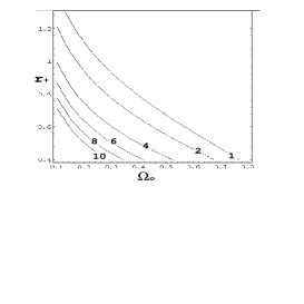
FIG. 1.: Level lines $\ell_{min}=(1,2,4,6,8,10)$ computed from (18) and (14) for the smallest CMB multipoles that can be generated in a universe with density parameter $\Omega_{0}$ and outradius $r_{+}$ in a theory where the perturbations are generated by TD. Note that this can only be an approximate guide.

III Conclusions

In this article, I have studied models where cosmological perturbations are generated by TD in a multi-connected universe. Given a cosmological model, i.e. ($\Omega_{0},r_{+}$), it can be concluded (modulo the approximations I have used) from Fig. 1 whether or not TD can account for the Sachs-Wolfe plateau observed by COBE. In a wide class of multi-connected universes, although TD may appear, they cannot explain COBE observations.

The conclusions rely on an important property of compact hyperbolic 3-manifolds (namely that their volume is a topological invariant, contrary to e.g. the 3-torus whose size is arbitrary) and on the “semi-topological” approximation which is a way to take into the topological constraints. I also restricted my analysis to the scalar modes, but the conclusion will be alike for vector and tensor modes since they are not generated after the time $\eta_{disp}$.

I am grateful to N. Deruelle for stimulating discussions and for helping me to improve this text. I also wish to thank P. Peter, D. Langlois, G. Faye and N. Cornish for their interesting remarks.

REFERENCES

- [1] A. Guth, Phys. Rev. 23, 347 (1981).
- [2] P.J. Steinhardt, “Cosmology at the crossroad”, Proceedings of the Snowmass Workshop on Particle Astrophysics and Cosmology, E. Kolb and R. Peccei Eds (1995).
- [3] T.W.B. Kibble, J. Math. Phys. A 9, 1387 (1976).
- [4] E.P.S. Shellard & A. Vilenkin, Cosmic strings and other topological defects, Cambridge University Press (1994).
- [5] http://map.gsfc.nasa.gov
- [6] http://astro.estec.esa.nl/SA-general/Projects/Cobras/
- [7] M. Lachièze-Rey & J.-P. Luminet, Phys. Rep. 254, 135 (1995).
- [8] J-P. Uzan, Int. Journal of Theor. Physics 36, 2167 (1997).
- [9] G.F.R. Ellis, Gen. Relativ. Gravitation 2, 7 (1971).
- [10] R. Lehoucq, M. Lachièze-Rey, J-P. Luminet, Astron. Astrophys. 313, 339 (1996).
- [11] D. Stevens, D. Scott & J. Silk, Phys. Rev. Lett. 71, 20 (1993); A. de Oliveira Costa, G.F. Smoot & A.A. Starobinsky, Ap.J. 468, 457 (1996).
- [12] J.J. Levin, J.D. Barrow, E.F. Bunn & J. Silk, Phys. Rev. Lett. 79, 974 (1997).
- [13] N.J. Cornish, D.N. Spergel & G.D. Starkman, gr-qc/9708225; Phys. Rev. Lett.77, 215 (1996).
- [14] N.J. Cornish, D.N. Spergel & G.D. Starkman, gr-qc/9602039; gr-qc/9708083.
- [15] G.D. Mostow, Ann. Math. Studies 78, Princeton University Press (1973);G. Prasad, Invent. Math. 21, 255 (1973).
- [16] J-P. Uzan & P. Peter, Phys. Lett. B406, 20 (1997).
- [17] W. Rindler, Mon. Not. R.A.S. 116, 663 (1956).
- [18] J. Weeks : http://www.geom.umn.edu:80/software.
- [19] C.J. Isham, Proc. R. Soc. London A362, 383 (1978).
- [20] N. Turok & D.N. Spergel, Phys. Rev. Lett. 64, 2736 (1990).
- [21] P.J.E Peebles, “Principles of Physical Cosmology”, Princeton University Press (1993).
- [22] G.F.R. Ellis, Proc. Int. Scool of Physics ‘Enrico Fermi’, course XLVII, ed. R.K. Sachs, NY academic Press, pp 104-79, (1971).
- [23] R.K. Sachs & A.M. Wolfe, Ap. J. 147, 73 (1967); M. Panek, Phys. Rev. D49, 648 (1986).
- [24] V.F. Mukhanov, F.A. Feldman & R.H. Brandenberger, Phys. Rep. 215, 203 (1992).
- [25] C.L. Bennet et al., Astrophys. J. 464, L1 (1994).
- [26] D. Lyth & A. Woszczyna, Phys. Rev. D52, 3338 (1995).
- [27] M. Kamionkowski & D.N. Spergel, Astrophys.J. 432, 7 (1994).
- [28] U.L. Pen, U. Seljak and N. Turok, Phys. Rev. Lett 79, 1615 (1997).
- [29] N. Deruelle, D. Langlois & J-P. Uzan, Phys. Rev. D56, 7608 (1997).