Uniformly accelerated sources in electromagnetism and gravity

Abstract

Electromagnetic field produced by magnetic multipoles in hyperbolic motion is derived and compared with electromagnetic field produced by electric multipoles in hyperbolic motion. The resulting fields are related by duality symmetry. Radiative properties of these solutions are demonstrated. In the second part an analogous, uniformly accelerated source of gravitational radiation is studied, within exact Einstein’s theory. Radiative characteristics of the corresponding solution as flux of the radiation and the total mass-energy of the system are calculated and graphically illustrated.

I Introduction

Because of nonlinearity of Einstein’s equations it is difficult to find their realistic exact radiative solutions. If we want to describe gravitational radiation from a given realistic source, we have to use various approximation methods, but then doubts arise if such approximate solutions correspond to some exact solutions.

It is easier to find exact solutions if we assume some symmetries. If we consider axially symmetric space-times which are asymptotically flat at least locally, the only second allowable symmetry that does not exclude radiation is the boost symmetry (see [1], [2]). Boost-rotation symmetric solutions describe ”uniformly accelerated particles” of various kinds and they contain gravitational radiation. These exact solutions help us to understand properties of gravitational radiation and they can also be used as tests of various approximation methods or numerical computations. In fact some specific boost-rotation symmetric solutions were used already as test beds in numerical relativity [3].

Gravitational radiation of uniformly accelerated particles and electromagnetic radiation of the analogous system of charges have some similar properties. In the first part of this paper we present new solutions of Maxwell equations describing uniformly accelerated magnetic multipoles, we compare them with solutions describing uniformly accelerated electric multipoles found in [4] (the case of monopole having been studied first by Born (1909)) and we analyze their radiative properties.

In the second part we turn the to boost-rotation symmetric solutions in general relativity. We analyze outgoing gravitational radiation from uniformly accelerated particles described by specific solutions and we calculate the mass decrease of the radiative system caused by energy carried out from the system by gravitational radiation.

II Electromagnetic fields and radiation patterns from magnetic multipoles in hyperbolic motion

A Construction of the solution

Assume that a particle with dipole magnetic moment $m_{0}$ moves with a uniform acceleration $\alpha^{-1}>0$ along the $z$-axis of cylindrical coordinates $(t,\rho,\phi,z)$ in Minkowski space-time. Its worldline is the hyperbola

$$\rho=0,\quad z=\sqrt{\alpha^{2}+t^{2}}.$$ (1)

If we want to calculate field produced by this particle we have to know corresponding four-current $J^{\alpha}$.

Electromagnetic field produced by magnetic dipole at rest is

$$\vec{A}={\frac{{\vec{m}_{0}}\times{\vec{r}}}{{r}^{3}}}.$$

Now we can use relation $\Delta\vec{A}=-4\pi\vec{\jmath}\,$ and calculate thus the corresponding current. If we apply $\partial_{z}$ on equation $\Delta({\frac{1}{r}})=-4\pi\delta(x)\delta(y)\delta(z)$, we obtain $\Delta({z}/{r}^{3})=4\pi\delta(x)\delta(y)\delta^{\prime}(z)$. We put $z$-axis in $m_{0}$-direction $\Rightarrow\vec{m}_{0}=[0,0,m_{0}]$, $\vec{m}_{0}\times\vec{r}=[-m_{0}y,m_{0}x,0]$ and we have

$$\vec{\jmath}_{\rm{rest}}={\it m_{0}}\,\delta(z)[\delta(x)\delta^{\prime}(y),-\delta^{\prime}(x)\delta(y),0].$$ (2)

A particle which is moving with velocity $v$ with respect to a coordinate system $S$ and has a magnetic dipole $m_{0}$ in its rest frame, in the frame $S$ has a magnetic dipole $m=m_{0}\sqrt{1-v^{2}}$. In the case of uniformly accelerated magnetic dipole we have $\sqrt{1-{v^{2}}}={\alpha}/{\sqrt{\alpha^{2}+t^{2}}}$ so the four-current of the uniformly accelerate magnetic dipole is

$$J^{\alpha}={\frac{{\it m_{0}}\,\alpha\,\delta(z-\sqrt{{\alpha}^{2}+{t}^{2}})}{\sqrt{{\alpha}^{2}+{t}^{2}}}}\ [0,\delta(x)\delta^{\prime}(y),-\delta^{\prime}(x)\delta(y),0]\ .$$ (3)

Corresponding four-potential can be found by using the standard relation

$$A^{\alpha}=\int\!{\frac{\delta(t^{\prime}+{{|\vec{x}-\vec{x}^{\prime}|}-t})}{|\vec{x}-\vec{x}^{\prime}|}}J^{\alpha}\,d^{3}x^{\prime}dt^{\prime}.$$ (4)

After quite a long calculation (details in [5]) we obtain the result which is most suitably expressed in cylindrical coordinates. We have $A^{t}=A^{z}=A^{\rho}=0$ and

$$A^{\phi}=\frac{4m_{0}\alpha(\alpha^{2}+\rho^{2}+z^{2}-t^{2})}{\xi^{3}}\,,\quad{\rm where}\quad\quad\xi=\sqrt{4\rho^{2}\alpha^{2}+(\alpha^{2}+t^{2}-z^{2}-\rho^{2})^{2}}\,,$$ (5)

but we will work in orthonormal tetrad basis defined by cylindrical coordinates; in this basis $A^{\alpha}$ has non-zero component $A^{(\phi)}=\rho A^{\phi}$. With the help of $\vec{B}=\nabla\times\vec{A}\ ,\quad\vec{E}=-\partial_{t}\vec{A}.$ we obtain $E^{(\rho)}=E^{(z)}=B^{(\phi)}=0$ and

$$B^{(\rho)} = \enspace\ 8m_{0}\rho z\partial_{\alpha}\left({\frac{{\alpha}^{2}}{{\xi}^{3}}}\right)\ ,$$ (6)

$$B^{(z)} = -4m_{0}\partial_{\alpha}\left({\frac{{\alpha}^{2}\left({\alpha}^{2}+{t}^{2}+{\rho}^{2}-{z}^{2}\right)}{{\xi}^{3}}}\right)\ ,\quad$$ (7)

$$E^{(\phi)} = -8m_{0}\rho t\partial_{\alpha}\left({\frac{{\alpha}^{2}}{{\xi}^{3}}}\right).$$ (8)

The field corresponding to a uniformly accelerated $2^{l}$-pole is given in terms of $(l-1)^{t}h$ derivatives with respect to the parameter $\alpha$ of the dipole fields. For detailed consideration in the case of electric multipoles see [4] (it is based on the way how dipole is constructed from monopoles etc., and on the fact that Maxwell equations are linear). In the case of magnetic multipoles we find

$$B^{(\rho)}_{(l)} = \enspace\ 8\frac{{\cal M}_{l}(2l-1)!!}{l!^{2}}\rho z\partial_{\alpha}^{(l)}\left({\frac{{\alpha}^{2}}{{\xi}^{3}}}\right)\ ,$$ (9)

$$B^{(z)}_{(l)} = -4\frac{{\cal M}_{l}(2l-1)!!}{l!^{2}}\partial_{\alpha}^{(l)}\left({\frac{{\alpha}^{2}\left({\alpha}^{2}+{t}^{2}+{\rho}^{2}-{z}^{2}\right)}{{\xi}^{3}}}\right)\ ,$$ (10)

$$E^{(\phi)}_{(l)} = -8\frac{{\cal M}_{l}(2l-1)!!}{l!^{2}}\rho t\partial_{\alpha}^{(l)}\left({\frac{{\alpha}^{2}}{{\xi}^{3}}}\right).$$ (11)

According to [4] we define ${\cal M}_{l}$ as the only one independent component of the corresponding multipole tensor up to a constant $l!^{2}/(2l-1)!!$. The field corresponding to uniformly accelerated electric multipoles ${\cal E}_{l}$ reads (see [4])

$$E^{(\rho)}_{(l)} = \enspace\ 8\frac{{\cal E}_{l}(2l-1)!!}{l!^{2}}\rho z\partial_{\alpha}^{(l)}\left({\frac{{\alpha}^{2}}{{\xi}^{3}}}\right)\ ,\quad$$ (12)

$$E^{(z)}_{(l)} = -4\frac{{\cal E}_{l}(2l-1)!!}{l!^{2}}\partial_{\alpha}^{(l)}\left({\frac{{\alpha}^{2}\left({\alpha}^{2}+{t}^{2}+{\rho}^{2}-{z}^{2}\right)}{{\xi}^{3}}}\right)\ ,$$ (13)

$$B^{(\phi)}_{(l)} = \enspace\ 8\frac{{\cal E}_{l}(2l-1)!!}{l!^{2}}\rho t\partial_{\alpha}^{(l)}\left({\frac{{\alpha}^{2}}{{\xi}^{3}}}\right).$$ (14)

We see that the field given by (10) can be obtained from that given by (13) by simple transformation

$$\vec{B}\rightarrow-\vec{E},\quad\vec{E}\rightarrow\vec{B}\ ,\quad{\cal E}_{l}\rightarrow{\cal M}_{l}.$$ (15)

It is a special case of duality symmetry (see for example [6]) which is well known in the vacuum case. To keep this symmetry in presence of charges, magnetic sources have to be introduced. Now the duality symmetry of Maxwell equations $(\vec{E}+i\vec{B})\rightarrow e^{i\Phi}(\vec{E}+i\vec{B})$ is restored if we also rotate the electric and magnetic charges $(q+ig)\rightarrow e^{i\Phi}(q+ig)$. We see that (15) is a special case of duality symmetry in the presence of charges.

The simplest example of fields (10) and (13) is the field of uniformly accelerated electric monopole (Born’s solution). This field has been studied in some basic works (Pauli 1918; Laue 1919) which considered the field as non-radiative. Even now some authors consider this solution as non-radiative [7]. This is in contradiction with expression according to which an accelerated charge radiates energy with the rate $(2/3)e^{2}{\dot{v}}^{2}$. If we expand the field strengths of Born’s solution in powers of $r^{-1}\ (r^{2}=\rho^{2}+z^{2})$, with the fixed time $t$, we find $\vec{E}\sim r^{-4}$, $\vec{B}\sim r^{-5}$ and thus Poynting vector $\vec{S}\sim r^{-9}$. In Figure 1 we can see that the quantities determining the field have the character of a pulse and it is therefore understandable why we find non-radiative Poynting vector $\vec{S}\sim r^{-9}$ when going to spatial infinity and therefore passing through a pulse. In the next part we will see that $\vec{S}\sim r^{-2}$ when travelling with the pulse with the velocity of light; then all fields (10) and (13) have radiative character.

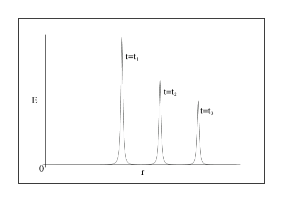
FIG. 1.: Pulse generated by uniformly accelerated electric charge ($E=|\vec{E}|$).

B Asymptotic behaviour and radiation properties

We will express the field components (10) in terms of spherical coordinates $(r,\theta,\varphi)$ and of the retarded time of the origin $u=t-r$ and expand them in $r^{-1}$ with $u$, $\theta$, $\phi$ fixed. Neglecting the terms $O(r^{-2})$ we find

$$B^{(\rho)} = \enspace\ {\cal M}_{l}G_{l}\sin\theta\cos\theta\frac{1}{r}\ ,$$ (16)

$$B^{(z)} = -{\cal M}_{l}G_{l}\sin^{2}\theta\frac{1}{r}\ ,$$ (17)

$$E^{(\phi)} = -{\cal M}_{l}G_{l}\sin\theta\frac{1}{r}\ ,$$ (18)

where

$$G_{l}=\frac{(2l-1)!!}{l!^{2}}\frac{\partial^{(l)}}{\partial\alpha}\frac{\alpha^{2}}{(u^{2}+\alpha^{2}\sin^{2}\theta)^{(3/2)}}\ .$$ (19)

From (17) we can calculate the leading term of the radial component of the Poynting vector $\vec{S}=(1/4\pi)\vec{E}\times\vec{B}$. Considering a particle with an arbitrary structure of electric and magnetic multipoles, we obtain

$$S_{r}=\frac{\sin^{2}\theta}{4\pi r^{2}}\sum_{l,l^{\prime}}({\cal E}_{l}{\cal E}_{l^{\prime}}+{\cal M}_{l}{\cal M}_{l^{\prime}})G_{l}G_{l^{\prime}}+O(r^{-3})\ .$$ (20)

Introducing the true retarded time $u^{*}$ of the particle with the help of the relation

$$t-u^{*}=|\vec{r}-\vec{r}^{\,*}|\ ,$$ (21)

where $(t,\vec{r})$ are the coordinates of an observation event and $(u^{*},\vec{r}^{\,*})$ are the coordinates of an emission event, we can write

$$u=u^{*}-\sqrt{{u^{*}}^{2}+\alpha^{2}}\cos\theta+O(r^{-1})\ .$$ (22)

Radial flux emitted at $u^{*}=0$ reads

$$S_{r}=\frac{\sin^{2}\theta}{4\pi r^{2}}\sum_{l,l^{\prime}}\frac{(2l-1)!!(2l^{\prime}-1)!!({\cal E}_{l}{\cal E}_{l^{\prime}}+{\cal M}_{l}{\cal M}_{l^{\prime}})}{l!^{2}l^{\prime}!^{2}}\frac{V_{l}V_{l^{\prime}}}{\alpha^{l+l^{\prime}+2}}\ ,$$ (23)

where $V_{l}$ can be obtained by substituting (22) and $u^{*}=0$ in

$$\alpha^{l+1}\,\frac{\partial^{(l)}}{\partial\alpha}\frac{\alpha^{2}}{(u^{2}+\alpha^{2}\sin^{2}\theta)^{(3/2)}}\ ;$$

thus $V_{0}=1$, $V_{1}=3\cos^{2}\theta-1$, $V_{2}=15\cos^{4}\theta-15\cos^{2}\theta+2$, $\dots$.
The total radiated power $R=2\pi\int_{0}^{\pi}{\lim\limits_{r\to\infty}}(r^{2}S_{r})\sin\theta\,{\rm d}\theta$ can be expressed in the form

$$R=\sum_{l,l^{\prime}}R^{(l,l^{\prime})}\frac{{\cal E}_{l}{\cal E}_{l^{\prime}}+{\cal M}_{l}{\cal M}_{l^{\prime}}}{{\alpha^{l+l^{\prime}+2}}}\ ,$$ (24)

with

$$R^{(l,l^{\prime})}=\frac{(2l-1)!!(2l^{\prime}-1)!!}{2l!^{2}l^{\prime}!^{2}}\int_{0}^{\pi}V_{l}V_{l^{\prime}}\sin^{3}\theta\,{\rm d}\theta\ ;$$ (25)

for all ${\cal M}_{l}=0$ (24) is identical with (23) in [4]. As in [4] we have $R^{(0,0)}=2/3$, $R^{(0,1)}=-4/15$, $R^{(1,1)}=8/21$ and so on. Due to the boost symmetry, the particles radiate out energy with a constant rate independent of $u^{*}$, and consequently with the same rate as at the turning point $u^{*}=0$. For the detailed consideration, see [8].

In terms of the electromagnetic field tensor, $F_{\mu\nu}$, we obtain, in coordinates $u$, $r$, $\theta$, $\phi$, the leading (in $r^{-1}$) radiative terms of a general boost-rotation symmetric electromagnetic field in the form:

$$F_{u\theta} = X=\frac{\epsilon(w)}{u^{2}}\ ,$$ (26)

$$F_{u\phi} = Y\sin\theta=\frac{\beta(w)\sin\theta}{u^{2}}$$ (28)

$${\rm with}\ \ w=\frac{\sin\theta}{u}\ ,$$

in which $X$ and $Y$ correspond to the so called news functions of the system, using the general-relativistic terminology (see [2]). (In cartesian coordinates these terms imply terms $\sim r^{-1}$.) For a uniformly accelerated electric monopole (i.e. Born’s solution) we obtain

$${\epsilon}(w) = \frac{{\cal E}_{0}\alpha^{2}w}{(1+\alpha^{2}w^{2})^{3/2}},$$ (29)

$${\beta}(w) = 0.$$ (30)

For a uniformly accelerated electric dipole we get

$${\epsilon}(w) = \frac{{\cal E}_{1}\alpha w(2-\alpha^{2}w^{2})}{(1+\alpha^{2}w^{2})^{5/2}}\ ,$$ (31)

$${\beta}(w) = 0\ ,$$ (32)

whereas for magnetic dipole one finds

$${\epsilon}(w) = 0\ ,$$ (33)

$${\beta}(w) = -\frac{{\cal M}_{1}\alpha w(2-\alpha^{2}w^{2})}{(1+\alpha^{2}w^{2})^{5/2}}\ .$$ (34)

For a general electric $2^{l}$-pole

$$\epsilon(w) = {\cal E}_{l}(G_{l}u^{3})w\ ,$$ (35)

$${\beta}(w) = 0\ ,$$ (36)

and for a magnetic $2^{l}$-pole

$${\epsilon}(w) = 0\ ,$$ (37)

$$\beta(w) = -{\cal M}_{l}(G_{l}u^{3})w\ ,$$ (38)

with $G_{l}$ given by (19).

III An example of radiative particles in general relativity

The Bonnor-Swaminarayan solution is a boost-rotation symmetric solution of Einstein’s equations. It describes the gravitational field around a finite number of monopole Curzon-Chazy particles uniformly accelerated in opposite directions. The acceleration force is caused by gravitational interaction among particles or by nodal singularities. The most interesting BS-solution contains two pairs of particles, there is one particle with positive and one with negative mass in each pair.

BS metric in cylindrical coordinates $t$, $\rho$, $z$ and $\phi$ reads

$$ds^{2}=-e^{\lambda}d\rho^{2}-\rho^{2}e^{-\mu}d\phi^{2}+\frac{1}{z^{2}-t^{2}}\Bigl{\{}(z^{2}e^{\mu}-t^{2}e^{\lambda})dt^{2}-(z^{2}e^{\lambda}-t^{2}e^{\mu})dz^{2}+2zt(e^{\lambda}-e^{\mu})dzdt\Bigr{\}}\ ,$$ (39)

in which functions entering the metric have forms

$$\mu = -\frac{2a_{1}}{R_{1}}-\frac{2a_{2}}{R_{2}}+\frac{2a_{1}}{h_{1}}+\frac{2a_{2}}{h_{2}}+\ln k\ ,$$ (40)

$$\lambda = \frac{a_{1}a_{2}}{(h_{1}-h_{2})^{2}}f-\rho^{2}(z^{2}-t^{2})(\frac{a_{1}^{2}}{R_{1}^{4}}+\frac{a_{2}^{2}}{R_{2}^{4}})+\frac{2a_{1}R}{h_{1}R_{1}}+\frac{2a_{2}R}{h_{2}R_{2}}+\ln k\ ,$$ (41)

$$R = \frac{1}{2}(\rho^{2}+z^{2}-t^{2})\ ,$$ (42)

$$R_{i} = \sqrt{(R-h_{i})^{2}+2\rho^{2}h_{i}}\ ,i=1,2\ ,$$ (43)

$$f = \frac{4}{R_{1}R_{2}}\Bigl{\{}\rho^{2}(z^{2}-t^{2})+(R-\rho^{2}-h_{1})(R-\rho^{2}-h_{2})-R_{1}R_{2}\Bigr{\}}\ ,$$ (44)

where $a_{1}$, $a_{2}$, $h_{1}>0$, $h_{2}>0$, $k>0$ are constants. In the case we are interested in, that is two pairs of freely moving positive and negative particles, we have

$$a_{1}=\frac{(h_{1}-h_{2})^{2}}{2h_{2}}\ ,\ a_{2}=-\frac{(h_{1}-h_{2})^{2}}{2h_{1}}\ ,\ k=1\ .$$ (45)

To examine the radiative properties and to find the news function of this solution it is necessary to transform the metric at first to spherical flat-space coordinates $\{R,\ \vartheta,\ \phi\}$ by $\rho=R\sin\vartheta$, $z=R\cos\vartheta$, $\phi=\phi$, and flat-space retarded time $U=t-R$ (see [8]) and then find a transformation to Bondi’s coordinates $u$, $r$, $\theta$ and $\phi$ (for details see [8] and [9]), in which the metric has Bondi’s form (see [2, 9] or (2), (4) in [8]). Bondi with collaborators discovered that these coordinates are most suitable for studying radiating systems. Coordinates $u$, $\theta$ and $\phi$ are such that they are stant and $r$ varies along outgoing null geodesics, i.e. light rays; the area of the surface element $u=$const, $r=$const is $r^{2}\sin\theta d\theta d\phi$ .

In our case of two freely falling particles in each pair in the limiting case of small masses ($h_{2}=h$, $h_{1}=h+\epsilon$, $\epsilon>0$ small, $k=1$ and masses are then $m^{(1)}=\epsilon^{2}/2h\sqrt{2h+2\epsilon}$, $m^{(2)}=-\epsilon^{2}/(2h+2\epsilon)\sqrt{2h}$) the relation between the flat coordinates $\{U,\ R,\ \vartheta,\ \phi\}$ and Bondi’s coordinates $\{u,\ r,\ \theta,\ \phi\}$ is (see [8])

$$U=\Bigl{(}u+O(\epsilon^{3})\Bigr{)}+O(1/r)\ ,\ R=r+O(1)\ ,\ \vartheta=\theta+O(1/r)\ ,\ \phi=\phi\ .$$ (46)

Then the news function in Bondi’s coordinates reads

$$c,_{u} = \epsilon^{3}\frac{3u\sin^{2}\theta}{2h(u^{2}+2h\sin^{2}\theta)^{\frac{5}{2}}}\ ,$$ (47)

$$= \epsilon^{3}\frac{3w^{2}}{2h(1+2hw^{2})^{\frac{5}{2}}}\frac{1}{u^{2}}\ {\rm{for}}\ u>0\ ,\ {\rm{where}}\ w=\frac{\sin\theta}{u}\ ,$$ (48)

$$= -\epsilon^{3}\frac{3w^{2}}{2h(1+2hw^{2})^{\frac{5}{2}}}\frac{1}{u^{2}}\ {\rm{for}}\ u<0\ .$$ (49)

As was shown in [2], a news function corresponding to any asymptotically flat boost-rotation symmetric solution of Einstein’s equations has to have a form $c,_{u}={\cal K}(w)/u^{2}$. Thus, for this case

$${\cal K}(w) = \epsilon^{3}\frac{3w^{2}}{2h(1+2hw^{2})^{\frac{5}{2}}}\ {\rm{for}}\ u>0\ ,$$ (50)

$${\cal K}(w) = -\epsilon^{3}\frac{3w^{2}}{2h(1+2hw^{2})^{\frac{5}{2}}}\ {\rm{for}}\ u<0\ .$$ (51)

We also need the news function to calculate the total mass of the system and to show how this mass decreases due to the emission of gravitational waves:

$$m = \frac{1}{4}\int_{0}^{\pi}(w^{2}{\cal K},_{w}),_{w}d\theta+\frac{1}{2}\int_{0}^{\pi}\frac{\lambda(w)}{w^{2}u^{2}}d\theta\ ,$$ (52)

$${\rm{where}}\quad\quad\quad\lambda(w),_{w} = w^{2}{\cal K},_{w}^{2}-\frac{1}{2w}(w^{3}{\cal K},_{ww}),_{w}\ .$$ (53)

Fairly long calculations lead to the total Bondi mass of the form

$$m = \frac{1}{4096}\frac{o^{2}u^{3}(5u^{4}+32u^{2}h+64h^{2})\sqrt{2}(-\ln(u^{2})+\ln\left|-2\sqrt{2h}\sqrt{u^{2}+2h}+u^{2}+4h\right|)}{h^{7/2}(u^{2}+2h)^{7/2}}$$ (54)

$$+\frac{1}{3072}\frac{o^{2}(u^{2}+4h)(15u^{4}+16u^{2}h+32h^{2})}{h^{3}u(u^{2}+2h)^{3}}\ ,\ \quad\quad\quad{\rm{where}}\ o=\frac{3\epsilon^{3}}{2h}\ .$$ (55)

In Figure 2 we see that $m$ as a function of $u$ is everywhere decreasing. The system does radiate gravitational waves.

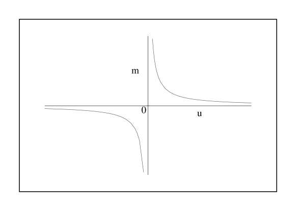
FIG. 2.: Decrease of the total mass-energy of the radiating system described by the metric (39)

FIG. 3.: Radiation pattern emitted at the turning point by particles described by the metric (39)

Acknowledgments
We thank J. Bičák for suggesting the problem and for constant encouragement. Thanks are also due to P. Bačkovský for stimulating discussions.

REFERENCES

• [1] J. Bičák and B. G. Schmidt, Isometries compatible with gravitational radiation, J. Math. Phys. 25(3), 600-606, (1984).
• [2] J. Bičák and A. Pravdová, Symmetries of asymptotically flat electrovacuum spacetimes and radiation, submitted to J. Math. Phys. (1998).
• [3] M. Alcubierre, C. Grundlach and F. Siebel, Integration of geodesics as a testbed for comparing exact and numerically generated spacetimes, in Abstr. ${\rm 15^{th}}$ Int. Conf. on Gen. Rel. Grav., (Pune 1997), p. 83.
• [4] J. Bičák and R. Muschall, Electromagnetic fields and radiation patterns from multipoles in hyperbolic motion, Wissenschaftliche Zeitschrift - der Friedrich-Schiller-Universita̋t Jena 39, 15 (1990).
• [5] V. Pravda, PhD dissertation, Department of Theoretical Physics, Charles University, Prague (1998).
• [6] Alvarez and Zamora, Duality in QFT, hep-th/9709180, (1997).
• [7] A. K. Singal, Radiation from a Charge Uniformly Accelerated for All Time, Gen. Rel. Grav., 29, 1371 (1997).
• [8] J. Bičák, Gravitational radiation from uniformly accelerated particles in general relativity, Proc. Roy. Soc. A 302, 201-224 (1968).
• [9] H. Bondi, M. G. J. van der Burg, and A. W. K. Metzner, Gravitational waves in general relativity VII. Waves from axi-symmetric isolated systems, Proc. Roy. Soc. A 269, 21 (1962);
R. K. Sachs, Gravitational waves in general relativity VII. Waves in asymptotically flat space-time, Proc. Roy. Soc. A 270, 103 (1962).