Abstract

I review recent developments in numerical relativity, focussing on progress made in 3D black hole evolution. Progress in development of black hole initial data, apparent horizon boundary conditions, adaptive mesh refinement, and characteristic evolution is highlighted, as well as full 3D simulations of colliding and distorted black holes. For true 3D distorted holes, with Cauchy evolution techniques, it is now possible to extract highly accurate, nonaxisymmetric waveforms from fully nonlinear simulations, which are verified by comparison to pertubration theory, and with characteristic techniques extremely long term evolutions of 3D black holes are now possible. I also discuss a new code designed for 3D numerical relativity, called Cactus, that will be made public.

1 Introduction

Numerical Relativity is having broad impact across many areas of relativity, astrophysics, and cosmology. Because of the pervasiveness of numerical techniques in relativity, it is simply impossible to survey the entire field in a plenary talk. Therefore, I will focus on a single area that cuts across many of these fields, and one which has galvanized the numerical relativity community: black holes (BH’s). This particular research illustrates many of the issues facing numerical relativists very well. Just to preview my overview of this subject, here is how I see the current status:

The Need. We need full 3D numerical relativity for gravitational wave astronomy. The imminent arrival of data from of the long awaited gravitational wave interferometers (see, e.g., Ref. [1] and references therein) has provided a sense of urgency in producing realistic simulations of strong sources of gravitational waves, possible only through the full machinery of numerical relativity. As has been emphasized by Flanagan and Hughes, one of the best candidates for early detection by the laser interferometer network is increasingly considered to be BH mergers[1, 2]. However, the signals are likely to be weak enough by the time they reach the detectors that reliable detection may be difficult without prior knowledge of the merger waveform. Flanagan’s talk in this volume reviews these issues in detail. These are among the reasons that the NSF-funded Binary Black Hole Grand Challenge Alliance has focused the efforts of numerous US and international groups on developing codes for solving the problem of 3D coalescing BH’s.

The Problems. There are many technical problems that must be solved before we can perform realistic simulations of BH merger events that will be useful for gravitational wave astronomy. I will provide a status report on the following issues: (a) The initial value problem. One must have initial data representing two astrophysically relevant BH’s orbiting each other in order to begin a simulation. (b) Boundary conditions. In any numerical code (with a finite boundary), boundary conditions are essential, and this is particularly true of the BH problem. Both the inner boundary, (say, inside the event horizon), and the outer boundary are problematic. (c) Adaptive mesh refinement. The computations of 3D relativity are so demanding that even on the world’s largest computers, one will have to resort to clever techniques to resolve numerically only those spacetime regions that demand it, or else the calculations will be intractable. Adaptive mesh refinement is being developed to refine the calculations only where it is needed.

The Goal: Waveforms. There are many reasons to pursue numerical relativity, even within the area of BH collisions (e.g. theoretical studies of the event horizons of dynamic BH’s can now be made through numerical relativity[3, 4, 5]). However, for gravitational wave astronomy, a most important goal of numerical relativity is the calculation of waveforms expected from the inspiral and merger. We will see that accurate waveforms from nonaxisymmetric BH simulations are already possible, even if they carry only a tiny fraction of the ADM mass in energy.

The Codes: Focusing Large Scale Efforts. In order to make real progress in 3D numerical relativity, one needs many skills. A wide range of difficult problems face us, ranging from mathematical formulations of the equations to advanced computational science techniques on parallel computers. Yet in the end a simulation must be performed by a single evolution code. For this reason, the efforts of many groups around the world have been focussed on the development of a small number of evolution codes. I will focus on one such 3D code, called Cactus, that is being used in many different projects, and will be made available to the community soon.

The Future: BH’s, Neutron Stars, The Universe. With so much activity on the rather narrow subject of BH’s to report on, there is unfortunately no room to discuss many other exciting areas in numerical relativity, such as critical phenomena, neutron star evolutions, and cosmology. But in summary, progress in this field is excellent, and we can look forward to many discoveries through numerical approaches to relativity in the future.

2 Initial Value Problem

In this section I review briefly the status of solving the initial value problem for BH’s. As with any initial data for Cauchy evolution in numerical relativity, the basic idea is to find relevant solutions to the Hamiltonian and momentum constraints that contain BH’s, and evolve them. As we will see in this section, the key difficulty lies in the word “relevant”; we now have at our disposal techniques to generate far more complicated datasets than we have the capability to actually evolve numerically.

I will not have space to review the formalism for developing initial data for numerical relativity. The standard article for this is still York’s classic[6]. (For relevant BH overviews, see also[7, 8, 9, 10, 11].) For notational purposes, the 3–metric is generally written as $ds^{2}=\psi^{4}\hat{ds}^{2}$ where $\hat{ds}^{2}$ is a known metric (often chosen to be the flat metric), and $ds^{2}$ is the unknown metric for which we are solving. Then the hamiltonian constraint is written as an elliptic equation for the unknown conformal factor $\psi$, which can be solved, given a solution for the extrinsic curvature $K_{ij}$ to the momentum constraints (e.g. time symmetric data, or $K_{ij}=0$). Once these data are given, they must be evolved, given a choice of lapse and shift.

2.1 Schwarzschild and Distorted Schwarzschild

The BH dataset most familiar to all relativists is the Schwarzschild solution. Although this spherical BH solution is now more than 80 years old, it is still an important solution to the constraints that is being used to test numerical relativity codes. When written in the notation of 3D numerical relativity, the 3–metric becomes

$$ds^{2}=\psi^{4}\hat{ds}^{2}\\ =\psi^{4}(dx^{2}+dy^{2}+dz^{2})\\ =(1+M/2r)^{4}(dx^{2}+dy^{2}+dz^{2})$$ (1)

where $r$ is the standard isotropic radius. This solution is still very relevant today, as any bound BH system without angular momentum (e.g., two BH’s colliding head on) must settle towards this solution at late times. With the standard Schwarzschild lapse this metric is the solution for all time, but with a dynamic slicing the 3–metric will evolve.

Now, imagine two BH’s colliding violently: merging at nearly the speed of light, their horizons combine to form a single, highly distorted BH. This BH must then settle down to its final equilibrium state. The Schwarzschild dataset was generalized to include such highly distorted, dynamic BH’s by numerous researchers, beginning in the 1980’s by Bernstein, Hobill, and Smarr. These datasets have been evolved in axisymmetry for a decade, and are now finding their way into full 3D simulations. They are very useful, since they allow one to explore the dynamics of distorted BH’s, such as those that will be formed during black hole collisions, without having to first evolve the inspiral. One simply starts with a distorted “Schwarzschild” (i.e., non-rotating) or “Kerr” (i.e., rotating) BH as initial data.

These datasets correspond to a gravitational wave of the form originally considered by Brill[12] superimposed on Schwarzschild. The flat conformal 3–metric $\hat{d}s^{2}$ is replaced by the “Brill” form with adjustable gravitational wave parameters. Such data sets mimic the state of two BH’s colliding, and form a useful model for studying the late stages of BH coalescence.

The 3–metric is $d\ell^{2}=\tilde{\psi}^{4}\left(e^{2q}\left(d\eta^{2}+d\theta^{2}\right)+\sin^{2}\theta d\phi^{2}\right),$where $\eta$ is a radial coordinate related to the Cartesian coordinates by $\sqrt{x^{2}+y^{2}+z^{2}}=e^{\eta}$. For details, please see[13]. Given a choice for the “Brill wave” function $q$, the Hamiltonian constraint leads to an elliptic equation for the conformal factor $\tilde{\psi}$. The function $q$ represents the gravitational wave surrounding the BH, and can be chosen freely to give a variety of distortion amplitudes and shapes (with some restrictions.) If the Brill wave amplitude vanishes, the undistorted Schwarzschild solution results, and for small amplitudes, the data corresponds to a perturbed BH. These data sets can also include angular momentum [14, 15], in which case the momentum constraints must also be solved. The rotating versions of these datasets build on the original rotating datasets of Bowen and York [16], which are contained as subsets of these more general datasets. Together, these datasets form a rich testing ground for BH evolution codes designed to treat the coalescence problem, as well as a laboratory for studying the dynamics of distorted BH’s. We will see results of evolutions of such BH data below.

2.2 Multiple BH Data

The datasets described above all have an Einstein-Rosen bridge construction: a simple wormhole connecting two identical asymptotically flat sheets. Such constructions were generalized over 30 years by Misner[17], Brill, Lindquist[18] and others to include two wormholes, leading to what we now know as two BH initial data. The Misner solution corresponds to two axisymmetric, equal mass BH’s, initially at rest (time symmetric initial data: $K_{ij}=0$). This is a single parameter family of initial data with an adjustable distance between the wormholes.

This family of initial data has become something of a classic in numerical relativity: the first attempt to evolve it numerically was by Hahn and Lindquist in 1963[19], even before the modern notions of BH’s or the ADM formalism had been fully developed. In the 1970’s DeWitt gave the problem to his student Larry Smarr, and along with Čadež and Eppley more modern numerical methods and slicing conditions were applied to the problem, this time with some success[20]. Again in the 1990’s, the same initial data were evolved again, this time with more powerful computers and numerical techniques, and at last reliable waveforms could be determined. This modern work also helped spark a renaissance of perturbative approaches to the problem, as outlined by Pullin in his plenary lecture. In sections below I will review recent numerical results in both axisymmetry and 3D. But the bottom line is that even these most simple possible BH collisions are still very challenging problems that continue to stress the most advanced numerical codes and computers we have!

However, we are ultimately interested in solving the more general 3D BH coalescence problem, with different masses, and with spin and orbital angular momentum. Techniques to create such initial datasets were developed by York and colleagues, especially Greg Cook. Generalizing the original ideas of Misner to create multiple wormhole datasets with two identical asymptotically flat sheets (i.e., there exists an isometry operator through the “throats” of the wormholes, mapping the top sheet to an identical one below), one can now generate full 3D datasets by solving both the momentum and Hamiltonian constraints[21]. A series of such initial datasets has been analyzed by Cook[22]. Generally the numerical solution is found only on one sheet, with the isometry operator providing boundary conditions on the throat. Mathematically straightforward, this can be painful to implement in 3D cartesian coordinates! An important variation on these techniques is the Brandt-Brügmann construction[23], which was only developed last year and evolved for the first time. Rather than an isometry surface, through which one universe is mapped to an identical one “below”, it has a singularity inside each hole that is built-in analytically. The numerical solution, for the nonsingular part, is then regular on the entire domain, which is very convenient to solve for in 3D cartesian coordinates.

The bottom line is that we have more initial sets than we can evolve right now! Full 3D data sets are ready, and waiting for us! However, the problems of evolution are far more difficult, as I will outline below. But even about the initial data, there is still a major caveat: although we can now generate very accurate binary BH initial data, with arbitrary spin and momenta, we really do not understand their connection to astrophysics well. The initial data will contain some gravitational wave content over which we have little control. Furthermore, how to match a given initial dataset to a particular inspiral scenario is unknown at present. So there is still much to be done even at the level of providing astrophysically relevant initial data.

3 The trouble with black holes

As I have described at length, we have many BH datasets at our disposal for evolution. But they all have in common one problem: singularities lurk within them, which must be handled numerically. Developing suitable techniques for doing so is one of the major research priorities of the community at present. If one attempts to evolve directly into the singularity, infinite curvature will be encountered, causing any numerical code to break down.

Traditionally, the singularity region is avoided by the use of “singularity avoiding” time slices, that wrap up around the singularity. Consider the evolution shown in Fig. 1. A star is collapsing, a singularity is forming, and time slices are shown which avoid the interior while still covering a large fraction of the spacetime where waves will be seen by a distant observer. However, these slicing conditions by themselves do not solve the problem; they merely serve to delay the onset of instabilities. As shown in Fig. 1, in the vicinity of the singularity these slicings inevitably contain a region of abrupt change near the horizon, and a region in which the constant time slices dip back deep into the past in some sense. This behavior typically manifests itself in the form of sharply peaked profiles in the spatial metric functions [24], “grid stretching” [25] or large coordinate shift [26] on the BH throat, etc. Numerical simulations will eventually crash due to these pathological properties of the slicing.

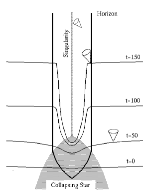
Figure 1.  : A spacetime diagram showing the formation of a BH, and time slices traditionally used to foliate the spacetime in traditional numerical relativity with singularity avoiding time slices. As the evolution proceeds, pathologically warped hypersurfaces develop, leading to unresolvable gradients that cause numerical codes to crash.

3.1 Apparent Horizon Boundary Conditions (AHBC)

Cosmic censorship suggests that in physical situations, singularities are hidden inside BH horizons. Because the region of spacetime inside the horizon is causally disconnected from the region of interest outside the horizon, one is tempted numerically to cut away the interior region containing the singularity, and evolve only the singularity-free region outside, as originally suggested by Unruh[27]. This has the consequence that there will be a region inside the horizon that simply has no numerical data. To an outside observer no information will be lost since the regions cut away are unobservable. Because the time slices will not need such sharp bends to the past, this procedure will drastically reduce the dynamic range, making it easier to maintain accuracy and stability. Since the singularity is removed from the numerical spacetime, there is in principle no physical reason why BH codes cannot be made to run indefinitely without crashing.

We spoke innocently about the BH horizon, but did not distinguish between the apparent and event horizon. These are very different concepts! While the event horizon, which is roughly a null surface that never reaches $\cal{I}$ and never hits the singularity, may hide singularities from the outside world in many situations, there is no guarantee that the apparent horizon, which is the (outermost) surface that has instantaneously zero expansion everywhere, even exists on a given slice! While methods for finding event horizons in numerical spacetimes are now known, and have been used to determine much interesting physics, they can only be found after examining the history of an evolution that has been already been carried out to sufficiently late times[3, 28]. Hence they are useless in providing boundaries as one integrates forward in time. On the other hand the apparent horizon, if it exists, can be found on any given slice by searching for closed 2–surfaces with zero expansion. Although one should worry that in a generic BH collision, one may evolve into situations where no apparent horizon actually exists, let us cross that bridge if we come to it!

Given these considerations, there are two basic ideas behind the implementation of the apparent horizon boundary condition:

(a) It is important to use a finite differencing scheme which respects the causal structure of the spacetime. Since the horizon is a one-way membrane, quantities on the horizon can be affected only by quantities outside but not inside the horizon: all quantities on the horizon can in principle be updated solely in terms of known quantities residing on or outside the horizon. There are various technical details and variations on this idea, which is called “Causal Differencing”[29] or “Causal Reconnection”[30], but here I focus primarily on the basic ideas and results obtained to date.

(b) A shift is used to control the motion of the horizon, and the behavior of the metric functions outside the BH.

An additional advantage to using causal differencing is that it allows one to follow the information flow to create grid points with proper data on them, as needed inside the horizon, even if they did not exist previously. (Remember above that we have cut away a region inside the horizon, so in fact we have no data there.) This process has been termed “educating grid points before birth” by Wai-Mo Suen. This will be an important education if one wants to let a BH move across the computational grid. If a BH is moving physically, it is also desirable for it to move through coordinate space. Otherwise, all physical movement will be determined by metric function evolution. For a single BH moving in a straight line, this may be reasonable, but for spiraling coalescence this will lead to hopelessly contorted grids. The immediate consequence of this is that as a BH moves across the grid, regions in the wake of the hole, now in its exterior, must have previously been inside it where no data exist! But with AHBC and causal differencing this need not be a problem.

Does the AHBC idea work? Preliminary indications are very promising. In spherical symmetry (1D), numerous studies show that one can successfully locate horizons, cut away the interior, and evolve for essentially unlimited times ($t\propto 10^{3-4}M$). The growth of metric functions can be completely controlled, errors are reduced to a very low level, and the results can be obtained with a large variety of shift and slicing conditions, and with matter falling in the BH to allow for true dynamics even in spherical symmetry[29, 31, 32, 33].

In 3D, the basic ideas are similar but the implementation is much more difficult. The first successful test of these ideas to a Schwarzschild BH in 3D used horizon excision and a shift provided from similar simulations carried out with a 1D code[34]. The errors were found to be greatly reduced when compared even to the 1D evolution with singularity avoiding slicings. (Another 3D implementation of the basic technique was provided by Brügmann [35].)

This was a proof of principle, but more general treatments are following. In collaboration with the NCSA/WashU group, Daues extended this work to a full range of shift conditions [36], including the full 3D minimal distortion shift [6]. He also applied these techniques to dynamic BH’s, including Misner data (where the holes are close enough together to be a single distorted Schwarzschild hole initially), and collapse of a 3D boson star to form a BH, at which point the horizon is detected, the region interior to the horizon excised, and the evolution continued with AHBC. The focus of this work has been on developing general gauge conditions for single BH’s without movement through a grid. Under these conditions, BH’s have been accurately evolved well beyond $t=100M$.

Taking the approach in a different direction, work of the Grand Challenge Alliance has been focussed on development of 3D AHBC techniques for boosted Schwarzschild BH’s[37]. In this work, analytic gauge conditions are provided, which are chosen to make the evolution static, although the numerical evolution is allowed to proceed freely. The boosted hole allows the first test of Suen’s “education of grid points before birth” as they emerge in the BH wake. Using causal differencing, this effort has successfully moved the BH several diameters across the grid, and accurate evolutions have now been carried out for $t\approx 500M$. In Fig. 2, recent results from such experiments are shown.

Figure 2.  : Metric component $g_{zz}$ along the $z$-axis is shown as a function of time for a boosted Schwarzschild BH evolved with AHBC. The flat region that moves diagonally to the right represents the excised region (inside the black hole). Note that points at the trailing edge (left side) are smoothly updated as the hole moves towards positive $z$.

These new results are significant achievements, and show that the basic techniques outlined above are not only sound, but are also practically realizable in a 3D numerical code. However, there is still a significant amount of work to be done! The techniques have yet to be applied carefully to distorted BH’s, with tests of the waveforms emitted (see below), they have not be applied to rotating BH’s of any kind, they have not been applied to colliding BH’s with horizon topology change, and moving black holes have yet to be evolved in AHBC with a nonanalytic gauge choice. There are still clearly many steps to be taken before the techniques will be successfully applied to the general BH merger problem.

4 Characteristic Evolution of 3D BH’s

Another very recent approach to 3D BH evolution that completely avoids the problems of grid stretching is characteristic evolution. The Pittsburgh group, in collaboration with the Grand Challenge Alliance, has developed the first full 3D characteristic code evolving nonlinear Einstein equations. This technique was originally envisioned as an approach to the problem of computing the spacetime in the far zone of the BH, where it would be matched to an interior Cauchy evolution code (Cauchy-Characteristic matching). In such an application, the characteristic portion of the spacetime would be foliated by outgoing null surfaces so that essentially outgoing radiation would be carried away to $\cal{I}$, but in this case it has been applied to the problem of evolving the BH’s themselves[38, 39]. The code uses the Bondi-Sachs form of the metric, and in the BH application evolves a region of spacetime from a region about $10M$ outside the horizon to the horizon itself, foliated by ingoing characteristic slices.

Using this technique, the characteristic code has successfully evolved 3D BH’s for essentially unlimited times ($t\approx 60,000M$). The results are even more impressive when one considers the fact that not only Schwarzschild BH’s were evolved, but also distorted and rotating BH’s. To my knowledge these are the first rotating BH’s to be evolved in 3D. The distorted BH’s consist of radiation imposed on the initial ingoing null surface, which then propagates in, hits the BH, and for the most part enter the horizon.

However, it seems likely that this method by itself will encounter difficulties for evolution of very highly distorted or colliding black holes, where focusing of ingoing light rays may create caustics, leading to a breakdown of the foliation. Also, ironically, the method is presently most successful when a BH is present, creating an $S^{2}\times R$ topology; dealing with the so-called $r=0$ problem is difficult for any formulation of the Einstein equations, and is avoided by using cartesian grids in the standard 3+1 formulations, but the characteristic method does not use cartesian grids, and would therefore have to face this problem in the absence of a BH (e.g., for the coalescence of neutron stars). Nonetheless, the possibility of very long time evolutions demonstrated with the characteristic evolution scheme is an exceptional achievement that seems likely to provide an alternate and superior approach for an interesting class of 3D BH spacetimes. It also provides strong evidence that characteristic evolution, when matched with a Cauchy interior evolution, should perform well.

5 3D Adaptive Mesh Refinement

3D BH simulations are very demanding computationally. In this section I outline the computational needs, and techniques designed to reduce them. We will need to resolve waves with wavelengths of order $5M$ or less, where $M$ is the mass of the BH. Although for Schwarzschild, the fundamental $\ell=2$ quasinormal mode wavelength is $16.8M$, higher modes, such as $\ell=4$ and above, have wavelengths of $8M$ and below. The BH itself has a radius of $2M$. More important, for very rapidly rotating Kerr BH’s, which are expected to be formed in realistic astrophysical BH coalescence, the modes are shifted down to significantly shorter wavelengths[2, 1]. As we need of order 20 grid zones to resolve a single wavelength, we can conservatively estimate a required grid resolution of about $\Delta x=\Delta y=\Delta z\approx 0.2M$. For simulations of time scales of order $t\propto 10^{2}-10^{3}M$, which will be required to follow coalescence, the outer boundary will probably be placed at a distance of roughly $R\propto 100M$ from the coalescence, requiring a Cartesian simulation domain of about $200M$ across. This leads to about $10^{3}$ grid zones in each dimension, or about $10^{9}$ grid zones in total. As 3D codes to solve the full Einstein equations have typically 100 variables to be stored at each location, and simulations are performed in double precision arithmetic, this leads to a memory requirement of order 1000 Gbytes! (In fairness to some groups that use spectral methods instead of finite differences (e.g., the Meudon group), I should point out highly accurate 3D simulations can now be achieved on problems that are well suited to such techniques, using much less memory! [40]).

The largest supercomputers available to scientific research communities today have only about $\frac{1}{20}$ of this capacity, and machines with such capacity will not be available for some years. Furthermore, if one needs to double the resolution in each direction for a more refined simulation, the memory requirements increase by an order of magnitude. Although such estimates will vary, depending on the ultimate effectiveness of inner or outer boundary treatments, gauge conditions, etc., they indicate that barring some unforeseen simplification, some form of adaptive mesh refinement (AMR) that places resolution only where it is required is not only desirable, but essential. The basic idea of AMR is to use some set of criteria to evaluate the quality of the solution on the present time step. If there are regions that require more resolution, then data are interpolated onto a finer grid in those regions; if less resolution is required, grid points are destroyed. Then the evolution proceeds to the next time step on this hierarchy of grids, where the process is repeated. These rough ideas have been refined and applied in many applications now in computational science.

There are several efforts ongoing in AMR for relativity. Choptuik was the early pioneer in this area, developing a 1D AMR system to handle the resolution requirements needed to follow scalar field collapse to a BH[41]. As an initially regular distribution of scalar field collapses, it will require more and more resolution as its density builds up. The grid density required to resolve the initial distribution may not even see the final BH. Further, as pulses of radiation propagate back out from the origin, they, too may have to be resolved in regions where there was previously a coarse grid. Choptuik’s AMR system, built on early work of Berger and Oliger[42], was able to track dynamically features that develop, enabling him to discover and accurately measure BH critical phenomena that have now become so widely studied[43].

Based on this success and others, and on the general considerations discussed above, full 3D AMR systems are under development to handle the much greater needs of solving the full set of 3D Einstein equations. A large collaboration, begun by the Grand Challenge Alliance, has been developing a system for distributing computing on large parallel machines, called Distributed Adapted Grid Hierarchies, or DAGH. Among other things, DAGH provides a framework for parallel AMR, and is one of the major computational science accomplishments to come out of the Alliance. Developed by Manish Parashar and Jim Browne, in collaboration with many subgroups within and without the Alliance, it is now being applied to many problems in science and engineering. One can find information about DAGH online at http://www.cs.utexas.edu/users/dagh/.

At least two other 3D software environments for AMR have been developed for relativity: one is called HLL, or Hierarchical Linked Lists, developed by Lee Wild and Bernard Schutz[44]; another, called BAM, was the first AMR application in 3D relativity developed by Brügmann [35], and will be discussed later. The HLL system has recently been applied to the test problem of the Zerilli equation describing perturbations of black holes[45]. As emphasized by Pullin in his GR15 talk, this nearly 30 year old linear equation is still providing a powerful model for studying BH collisions, and it is also being used as a model problem for 3D AMR. In this work, the 1D Zerilli equation is recast as a 3D equation in cartesian coordinates, and evolved within the AMR system provided by HLL. Even though the 3D Zerilli equation is a single linear equation, it is quite demanding in terms of resolution requirements, and without AMR it is extremely difficult to resolve both the initial pulse of radiation, the blue shifting of waves as they approach the horizon, and the scattering of radiation, including the normal modes, far from the hole. In Fig. 3 I show results obtained using this system. The effect of the AMR is impressive, allowing one to capture the physics accurately even when the “base grid”, which is the coarsest resolution level, is completely inadequate to resolve the physically interesting features.

Figure 3.  : Tracking of outgoing waves using one and two levels of dynamic refinement. The signal shown is seen by an equatorial observer located at 125M. The base grid resolution is 2M. Using one level of refinement captures and contains the first two outgoing modes (dotted line) compared to the the 1D result (solid line). The quality of the signal improves even more when two levels of dynamic refinement are used (dashed line).

6 Outer Boundary Treatments

Appropriate conditions for the outer boundary have yet to be derived for 3D. In 1D and 2D codes, the outer boundary is simply placed far enough away that the spacetime is nearly flat there, and static or flat boundary conditions can usually be specified for the evolved functions. However, due to the constraints placed on us by limited computer memory, this is not currently possible in 3D. AMR will be of great use in this regard, but will not substitute for proper physical treatment. Most results to date have been computed with the evolved functions kept static at the outer boundary, even if the boundaries are too close for comfort in 3D!

There are several other approaches under development that promise to improve this situation greatly that I will not have room to explore in detail here, but should be mentioned. Generally, one has in mind using Cauchy evolution in the strong field, interior region where the BH’s are colliding. This outer part of this region will be matched to some exterior treatment designed to handle what is primarily expected to be outgoing radiation.

Two major approaches have been developed by the Grand Challenge Alliance and other groups. First, by using perturbation theory, as described later in this paper, it is possible to identify quantities in the numerically evolved metric functions that obey the Regge-Wheeler and Zerilli wave equations. These can be used to provide boundary conditions on the metric and extrinsic curvature functions in an actual evolution, as described in a recent paper from the Grand Challenge Alliance [46]. This is an excellent step forward in outer boundary treatments that should work to minimize reflections of the outgoing wave signals from the outer boundary. In tests with weak waves, a full 3D Cauchy evolution code has been successfully matched to the perturbative treatment at the boundary, permitting waves to escape from the interior region with very little reflection. Alternatively, “Cauchy-Characteristic matching” attempts to match spacelike slices in the Cauchy region to null slices at some finite radius, and the null slices can be carried out to $\cal{I}$. As described above, the full 3D characteristic evolution codes have progressed dramatically in recent years, and although the full 3D matching remains to be completed, tests of the scheme in specialized settings show promise[47]. One can also use the hyperbolic formulations of the Einstein equations to find eigenfields, for which outgoing conditions can in principle be applied[48]. In 3D this technique is still under development, but it exploits mathematical properties of the equations, and 1D tests work well, it shows promise for future work. Finally, another hyperbolic approach uses conformal rescaling to move the boundary to infinity [49, 50, 51, 52]. These methods have different strengths and weaknesses, but all promise to improve boundary treatments significantly, helping to enable longer evolutions than are presently possible.

7 3D Dynamic BH Simulations

I now turn to what has actually been achieved over the last few years in actual 3D BH evolutions in a Cauchy evolution setting, which is expected to be the main line of attack for the general binary BH merger problem. Although I have discussed many techniques above that are thought to be needed for the general problem, such as AMR, AHBC, advanced boundary treatments, and so on, in this section I discuss what has already been possible without such advanced algorithms.

In what follows, I discuss a series of simulations carried out in 3D cartesian coordinates with a fixed, 3D mesh (implying that resolution is very limited, even on the world largest supercomputers), with standard singularity avoiding slicings instead of AHBC (implying that slices will become pathologically warped, causing the codes to crash), and with fixed outer boundaries (implying that waves that reach the boundary will be reflected back into the domain of interest). In spite of all of these caveats, we will see that already one can achieve quite remarkable results in 3D, which can be verified through a series of testbed and convergence calculations. As advanced algorithms are developed, they will be tested on simulations such as these, and should extend our capabilities with each step forward.

7.1 Distorted BH’s: 3D Spectroscopy

I begin with a simulation of a distorted single BH in a 3D code, with an initial data set of the “Brill wave plus BH” type discussed above. One can consider this as a prototype of a black hole just formed during the collision process of two merging black holes. The goal here is to see if one can evolve it properly in a full 3D code, track the waves emitted as it settles down, and extract them from the metric functions actually being evolved.

As an example of the type of initial data under consideration, I first show in Fig. 4 an embedding diagram of the apparent horizon of such a hole. In this case, I show an axisymmetric hole, because the horizon embeddings are easy to compute, but below I will consider evolutions for both axisymmetric and full 3D BH initial data.

Figure 4.  : We show the embedding diagram for the apparent horizon of an axisymmetric, highly distorted BH initial dataset. Embedding coordinates are normalized by the square root of the area. Such a BH is similar in shape to BH’s formed during the head-on collision of two black holes, and is a useful test case for 3D numerical evolution.

The 3D code, developed originally by the NCSA/WashU/Potsdam collaboration, and developed further for these simulations by Karen Camarda, is written without making use of any symmetry assumptions. The code is a general 3D ADM code (the so-called “G” code), allowing very general slicings and shift conditions, but the particular simulations shown here use zero shift and a particular singularity avoiding slicing described in Ref. [13, 53]. The initial data I discuss here have both equatorial plane symmetry and quadrant symmetry (i.e., although fully 3D, any intrinsic $\phi-$dependence is repeated in each quadrant). Hence we can save on the memory and computation required by evolving only one octant of the system. As discussed above, without some form of memory savings, highly resolved, 3D simulations with outer boundaries sufficiently far away are simply not possible on even the largest available computers in 1997. As shown in [34], this trick has no effect on the simulations except to reduce the computational requirements by a factor of eight. Even with such computational savings, these are extravagant calculations! The results presented in this paper were computed on a 3D Cartesian grid of $300^{3}$ numerical grid zones, take about 12 Gbytes of memory, and require about a day on a 128 processor, SGI/Cray Origin 2000 parallel supercomputer.

The questions we want to answer with these simulations are: (a) Can we evolve highly distorted BH’s, like those formed in a collision, in a general 3D simulation code?; (b) Can we extract radiation, even when the waves are very weak, with energy $E<10^{-3}M$?; (c) Do we know if we get the right answer? The answer to all three questions is an emphatic YES!. By using a combination of 2D codes and perturbative testbeds, we will see that even very weak $\ell-$modes, including nonaxisymmetric $\ell=4$ modes, can be very accurately obtained in a full 3D cartesian simulation. For this reason, I like to refer to this as BH spectroscopy! Many energy levels of the BH excitations (quasinormal modes) can be followed and studied in full 3D.

There are many ways to evolve such a distorted BH system, and I will discuss and compare three of them here: (a) perturbative evolution, (b) axisymmetric evolution in the case where there is no $\phi$ dependence, and (c) full 3D evolution as above.

Comparison with results from mature 2D codes.

Over the last decade, very mature 2D codes have been developed and well tested. These codes have been applied to distorted Schwarzschild [54], Misner colliding black holes [55, 56], and distorted rotating black holes [57]. They provide an excellent testing ground for full 3D evolutions, as one can transform the initial data sets into Cartesian coordinates, and evolve them as full 3D data sets, even though the underlying initial data are axisymmetric. As the 2D and 3D codes use completely different coordinate systems, gauges, slicings, etc., even the metric functions that are evolved will be very different: only the physics should be the same in both codes.

One particular measure of the physics, which is most appropriate for gravitational wave astronomy, is a waveform seen by a distant observer. This can be computed using an extraction technique developed originally by Abrahams[58, 59]. This technique is based on a gauge-invariant perturbation theory developed by Moncrief [60], and in the present 3D application is detailed in Refs.[61, 53, 62]. Essentially, the Zerilli function $\psi$, which obeys the Zerilli wave equation discussed above, is computed as a function of time at various radii away from the distorted BH.

As an example of such simulations, we study the evolution of the distorted single BH initial data set, similar to the one whose horizon embedding is shown above ($(a,b,w,n,c)=(0.5,0,1,2,0)$ in the language of Ref. [53]). In Fig. 5a we show the result of the 3D evolution, focusing on the $\ell=2$ Zerilli function extracted at a radius $r=8.7M$ as a function of time. Superimposed on this plot is the same function computed during the evolution of the same initial data set with a 2D code, based on the one described in detail in [54, 63]. The agreement of the two plots is quite remarkable. It is important to emphasize that the two results were computed with different slicings, different coordinate systems, and different spatial gauges. Yet the physical results obtained by these two different numerical codes, as measured by the waveforms, are remarkably similar (as one would hope). A full evolution with the 2D code to $t=100M$, by which time the hole has settled down to Schwarzschild, shows that the energy emitted in this mode at that time is about $4\times 10^{-3}M$. This result shows that now it is possible in full 3D numerical relativity, in cartesian coordinates, to study the evolution and waveforms emitted from highly distorted BH’s, even when the final waves leaving the system carry a small amount of energy.

In Fig. 5b we show the $\ell=4$ Zerilli function extracted at the same radius, computed during evolutions with 2D and 3D codes. This waveform is more difficult to extract, because it has a higher frequency in both its angular and radial dependence, and it has a much lower amplitude: the energy emitted in this mode is three orders of magnitude smaller than the energy emitted in the $\ell=2$ mode, i.e., $10^{-6}M$, yet it can still be accurately evolved and extracted. This is quite a remarkable result, and bodes well for the ability of numerical relativity codes ultimately to compute accurate waveforms, which are buried deeply in the metric functions actually evolved, that will be of great use in interpreting data collected by gravitational wave detectors. (However, as I point out below, there is a quite a long way to go before the general 3D coalescence can be studied!)

Figure 5.  : We show the (a) $\ell=2$ and (b) $\ell=4$ Zerilli functions vs. time, extracted during 2D and 3D evolutions of the data set $(a,b,w,n,c)=(0.5,0,1,2,0)$. The functions were extracted at a radius of $8.7M$. The 2D data were obtained with $202\times 54$ grid points, giving a resolution of $\Delta\eta=\Delta\theta=0.03$. The 3D data were obtained using $300^{3}$ grid points and a resolution of $\Delta x=0.0816M$.

Comparison against full 3D perturbative evolution

After passing tests of 3D evolution of axisymmetric distorted black hole initial data, we now turn to full 3D distorted BH data sets, for which there are no axisymmetric treatments available for comparison. However, if distortions are fairly small, one expects that the initial data can be evolved by perturbation theory. As Pullin describes in detail in this volume, this approach has been remarkably successful in handling a variety of BH systems. The approach is similar to that used above to extract the waveforms, except that in this case the Zerilli function is computed throughout the spatial domain in the back hole initial data. This provides Cauchy data for the Zerilli evolution equation, which can then be used to evolve all $\ell-$modes forward in time. The results can then be compared with the full nonlinear evolution, which is analyzed using the gauge-invariant waveform extraction procedure described above. If all is well, and the evolutions are truly in the perturbative regime, the results should agree.

In Fig. 6 I show the results of one such comparison. A 3D BH is evolved with the full 3D nonlinear code described above. The waveform is extracted from the simulation, and compared to the results of the perturbative evolution. The mode shown in Fig. 6a is the nonaxisymmetric $\ell=m=2$ mode, already described above as one of the most relevant for gravitational wave astronomy. The waveform in Fig. 6b is the higher order $\ell=4,m=2$ mode, which carries much lower energy. These results have been reported in much more detail in [61, 13, 62, 64].

Figure 6.  : We show waveforms for the (a) $\ell=m=2$ and (b) $\ell=4,m=2$ nonaxisymmetric modes extracted from the full nonlinear simulation of a 3D distorted BH. Solid lines show the nonlinear evolutions, and the dotted lines show the perturbative results.

To summarize these results: In recent years great progress has been made in full 3D numerical relativity applications to BH evolutions. We can now evolve 3D distorted BH’s, with standard slicing techniques, long enough to track the development of the radiation patterns emitted during the ringdown of the BH. This is the first time that true 3D BH’s have been evolved in full numerical relativity, and the perturbative results confirm that even the minute details of the spectrum of gravitational radiation emitted, carrying energy of order $10^{-6}M$, are accurate. Although there are still many long steps to the general coalescence problem, for this class of test problems, I think it is fair to say that 3D numerical relativity has progressed from blunt instrument to fine art: 3D BH spectroscopy is now possible!

7.2 First 3D Collision of 2 BH’s

Now I move on to the problem of two colliding BH’s, which is the long term goal. This is a much harder problem that will ultimately require the advanced techniques under development, such as AHBC, AMR, advanced BC’s, etc, but as always there are simpler stepping stones to the general merger system. We take the Misner data as our prototype BH collision, and see what is possible in 3D. As discussed above, the Misner two BH data has played a central role in numerical relativity for more than three decades. Through extensive axisymmetric simulations [55, 56, 65], perturbation theory (Pullin’s lecture), and horizon studies[3], this is a true two BH system that is understood in great detail.

We have also computed the head-on collision of two equal mass black holes in the 3D code. Preliminary results agree very well with 2D, although we cannot yet evolve the 3D system as far into the future. In Fig. 7 I show the evolution of the radiation field $\Psi_{4}$ as a grayscale map, and the coordinate position of the event horizon, traced out using the techniques described above. Notice the “banana” shaped quadrupole lobes of radiation propagating out from the colliding holes, just as in the 2D calculations. Quantitative studies of the coalescence time of the horizons also show excellent agreement with the 2D studies[66].

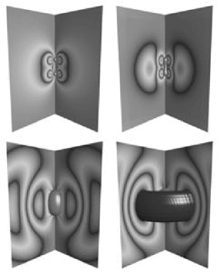
Figure 7.  : 3D Evolution of the head-on collision of two black holes. The radiation field $\Psi_{4}$ is shown as a grayscale map. The event horizon is shown as a solid object in the center. Features compared to the results obtained in 2D evolutions show good agreement.

This work is already more than two years old, but shows what is possible at present even without advanced techniques such as AHBC and AMR, and that for highly dynamic colliding BH spacetimes, 3D calculations are capable of producing waveforms and horizon dynamics. These calculations are now being redone with new codes (see below), and bigger computers, and should yield more accurate and detailed results. Further, 3D calculations such as these will provide important testbeds for the more advanced techniques as they are developed.

This is exciting progress, but there is still a long way to go! Up to this point, important features, such as orbital angular momentum, have not been considered. We turn to the general binary merger case next.

7.3 First true 3D BH Collision Simulation

The first attempt to test out the general 3D binary BH data in an evolution code was recently made by Brügmann [67]. Using an ADM 3D code (BAM, independent of the one used in the above simulations), he recently evolved a true 3D binary BH dataset, with spin and angular momentum, going beyond single distorted 3D BH’s and simplified axisymmetric BH collisions. The datasets he evolved belong to the new family of “Black Hole Punctures” [23], the generalization of multiple Schwarzschild holes with singularities, as described above.

As in the above simulations, he used a “traditional” evolution approach: a 3D Cartesian grid, no shift, maximal slicing to avoid singularities, no AHBC, and fixed outer boundaries. As discussed above, such simulations are extremely demanding computationally. The results of the preceding section were achieved by making use of certain symmetries to reduce the computational domain required, but with these general data sets, no such reduction is possible. The entire domain must be evolved. In this case, one must resort to some form of adaptive computation in order to reasonably resolve the BH’s and place the boundary reasonably far away.

Rather than employing a fully adaptive grid, which requires still some development, he employed a series of nested grids, each interior grid having higher resolution than the one that contains it. This way one can achieve high resolution in the central region where BH’s are merging, while placing the boundaries far away, in regions where one can afford to have rather coarse resolution. Without such techniques, these calculations would be impossible. Another innovative feature of this work is the coupling of maximal slicing, an elliptic equation, to the evolution equations, in the presence of nested grids. This a very difficult computational problem, and is perhaps the first successful implementation in 3D relativity.

The results show the strength of this technique: although the simulations could not be followed far into the future, it was possible to determine the location of the initial 3D apparent horizons, and to track the development of a global apparent horizon, indicating that the individual holes had merged, at a later time. A snapshot of this simulation in shown in Fig. 8, where one can see the two individual holes embedded in a larger horizon that developed towards the end of the simulation.

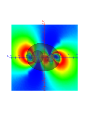
Figure 8.  : A snapshot of true 3D binary BH evolution, showing the merging of two apparent horizons, shown inside the final horizon, the transparent surface engulfing them. The grayscale map shows the metric function $g_{zz}$.

While very preliminary, this calculation gives a glimpse of what will be possible in the future. It is reminiscent of the early 2D simulations of Smarr and Eppley [68], when crude features of the Misner BH spacetime could be seen, but refined details, such as clean waveforms, would require still more development of numerical relativity techniques. With each advance in algorithm technology, more sophisticated problems are being attacked, leading towards realistic astrophysical BH merger simulations.

8 Putting the Pieces Together: Codes for 3D Relativity

As one can see, the solution to a single problem in numerical relativity requires a huge range of computational and mathematical techniques. It is truly a large scale effort, involving experts in computer and computational science, mathematical relativity, astrophysics, and so on. For these reasons, aided by collaborations such as the Grand Challenge Alliance, there has been a great focusing of effort over the last years.

A natural byproduct of this focusing has been the development of codes that are used and extended by large groups. A code must have a large arsenal of modules at its disposal: different initial data sets, gauge conditions, horizon finders, slicing conditions, waveform extraction, elliptic equation solvers, AMR systems, boundary modules, different evolution modules, etc. Furthermore, these codes must run efficiently on the most advanced supercomputers available. Clearly, the development of such a sophisticated code is beyond any single person or group. In fact, it is beyond the capability of a single community! Different research communities, from computer science, physics, and astrophysics, must work together to develop such a code.

As an example of such a project, I describe briefly the “Cactus” code, developed by a large international collaboration[69]. This code is an outgrowth of the last 5 years of 3D numerical relativity development primarily at NCSA/Potsdam/WashU, and builds heavily on the experience gained in developing the so-called “G” and “H” codes [34, 70, 69]. The core of Cactus was written from the ground up during 1997 by Paul Walker and Joan Massó, and then heavily developed by the entire groups at Potsdam, WashU and NCSA. Presently, it is being developed collaboratively by these groups in collaboration with groups at Palma, Valencia, PRL in India, and computational science groups at U. of Illinois, and Argonne National Lab.

The code has a very modular structure, allowing different physics, analysis, and computational science modules to be plugged in. In fact, versions of essentially all the modules listed above are already developed for the code. For example, several formulations of Einstein’s equations, including the ADM formalism and the Bona-Massó hyperbolic formulation, can be chosen as input parameters, as can different gauge conditions, horizon finders, hydrodynamics evolvers, etc. It is being tested on BH spacetimes, such as those described above, as well as on pure wave spacetimes, self-gravitating scalar fields and hydrodynamics. It has also been designed to connect to DAGH ultimately for parallel AMR.

The code has also been heavily optimized to take advantage of the most powerful parallel supercomputers. With help of experts at Cray and SGI, the code has recently achieved 100Gflops (100 billion floating point operations per second) on a 768 node Cray T3E, making it one the fastest general purpose production codes available in any area of scientific computing.

This code was also designed as a community code. After first developing and testing it within our rather large community of collaborators, it will be made available with full documentation via a public ftp server maintained at AEI. By having an entire research community using and contributing to such a code, we hope to accelerate the maturation of numerical relativity. Information about the code is available online, and can be accessed at http://cactus.aei-potsdam.mpg.de.

9 Summary

To conclude, it is clear that 3D numerical relativity has had many successes over the last years, but that it also requires further development of basic algorithms before it will be able to solve fully such complex problems as the general merger of two spiraling black holes. We have extensive families of BH initial data ready for evolution, and even with presently limited computational techniques it has been shown that highly accurate nonaxisymmetric waveforms can be obtained from simulations of fully 3D distorted black holes (black hole spectroscopy!) and head-on collisions of black holes, and that one can already crudely study the merger of general binary BH’s for limited times. Further, characteristic evolution in 3D has made truly dramatic progress in the last year.

Extending our capabilities of highly accurate waveforms to true 3D BH mergers, with orbital angular momentum, will require the further development of advanced computational and algorithm techniques, including apparent horizon boundary conditions, adaptive mesh refinement, improved outer boundary conditions, perhaps through Cauchy-characteristic or perturbative matching, and a better understanding of gauge conditions (Gauge conditions are a major research area that I have not discussed, but one which will require a great deal of attention). This is a tall order, but I have shown that in almost each area, dramatic progress has been made in the last few years. AHBC has successfully employed general gauge conditions in one case to evolve a dynamic but nonmoving BH, and has also been used successfully to allow a boosted Schwarzschild hole to move across a 3D grid. Full 3D AMR techniques have been demonstrated for model problems such as the 3D Zerilli equation to capture accurately the physics that would otherwise be unattainable with a 3D uniform grid code. Large scale simulation codes, such as Cactus and the Grand Challenge Alliance codes, are under development by large collaborations, with the goal of integrating all these pieces for a unified attack on this problem.

I have discussed the important role played by testbeds in this work, but want to stress the powerful impact that collaborations with our colleagues in perturbation theory has had. Fortunately, Jorge Pullin has covered this in his contribution. I believe this rebirth of perturbative approaches to understanding BH interactions will continue to play a central in both the verification of numerical relativity and in the physical understanding and interpretation of the results.

I have focussed on black hole evolutions, and have had to leave out discussion of a large number of other topics central to numerical relativity that really deserve to be covered. For example, there has been much talk about hyperbolic systems in numerical work over the last few years, and I regret not having space to discuss that here. The field is still very much alive, and the hopes that hyperbolic formulations will allow a superior numerical treatment and a deeper understanding of the Einstein equations are undamped. In fact, a major motivation for the Cactus code was to provide a single framework for developing and comparing hyperbolic formulations with standard ADM formulations on a variety of problems, and I expect much work on this subject to continue to be published in the coming years.

Another major topic that has received no mention is work on coalescing neutron stars, another important source of gravitational waves. Several large scale efforts are underway to attack this problem, including a long term Japanese effort [71] and a NASA funded Grand Challenge effort involving researchers at 6 institutions in the US and Germany (http://wugrav.wustl.edu/nsnsgc/nsnsgc.html). The Cactus code is also playing a central role in the latter collaboration.

I hope it is clear that although there is much work to be done, 3D numerical relativity is improving rapidly, and that many exciting results are possible already, even with still limited computers and techniques available. But even in those areas under development, we have a roadmap to address the problems we are facing, and the prognosis for improvement is excellent!

10 Acknowledgments

I would like to thank the organizers for inviting me to give this overview of current work in numerical relativity. The work reviewed here in which I have been personally involved has been the result of a wonderful collaboration between the members of my groups at Illinois and Potsdam, the group led by Wai-Mo Suen at Washington University, and various other groups around the world. Some of the work reviewed here was supported by grants NSF PHY/ASC 93–18152 (ARPA supplemented) and NASA-NCCS5-153. Thanks also go to Miguel Alcubierre, Bernd Brügmann, Harry Dimmelmeier, Gerd Lanfermann, Tom Goodale, and Ryoji Takahashi for carefully reviewing the paper.

References

- [1] Éanna É. Flanagan and S. A. Hughes, Phys. Rev. D 57, 4566 (1998), gr-qc/9710129.
- [2] Éanna É. Flanagan and S. A. Hughes, Phys. Rev. D 57, 4535 (1998), gr-qc/9701039.
- [3] P. Anninos, D. Bernstein, S. Brandt, J. Libson, J. Massó, E. Seidel, L. Smarr, W.-M. Suen, and P. Walker, Phys. Rev. Lett. 74, 630 (1995).
- [4] R. Matzner, E. Seidel, S. Shapiro, L. Smarr, W.-M. Suen, S. Teukolsky, and J. Winicour, Science 270, 941 (1995).
- [5] S. Shapiro, S. Teukolsky, and J. Winicour, Phys. Rev. D 52, (1995).
- [6] J. York, in Sources of Gravitational Radiation, edited by L. Smarr (Cambridge University Press, Cambridge, England, 1979).
- [7] E. Seidel, in Relativity and Scientific Computing, edited by F. Hehl (Springer-Verlag, Berlin, Germany, 1996).
- [8] E. Seidel and W.-M. Suen, in Relativistic Gravitation and Gravitational Radiation, edited by J.-P. Lasota and J.-A. Marck (Cambridge University Press, Cambridge, England, 1997), pp. 335–360.
- [9] E. Seidel, in Gravitation and Cosmology, edited by S. Dhurandhar and T. Padmanabhan (Kluwer Academic, Dordrecht, 1997), pp. 125–144.
- [10] E. Seidel and W.-M. Suen, Acta Helvetica 69, 454 (1996).
- [11] E. Seidel, in On the Black Hole Trail, edited by B. Iyer and B. Bhawal (Kluwer, 1998).
- [12] D. S. Brill, Ann. Phys. 7, 466 (1959).
- [13] K. Camarda and E. Seidel, Phys. Rev. D 57, R3204 (1998), gr-qc/9709075.
- [14] S. Brandt, K. Camarda, and E. Seidel, in preparation for Phys. Rev. D.
- [15] S. Brandt, K. Camarda, and E. Seidel, in Proc. 8th M. Grossmann Meeting, edited by T. Piran (World Scientific, Singapore, 1998), in press.
- [16] J. Bowen and J. W. York, Phys. Rev. D 21, 2047 (1980).
- [17] C. Misner, Phys. Rev. 118, 1110 (1960).
- [18] D. S. Brill and R. W. Lindquist, Phys. Rev. 131, 471 (1963).
- [19] S. G. Hahn and R. W. Lindquist, Ann. Phys. 29, 304 (1964).
- [20] L. Smarr, Ann. N. Y. Acad. Sci. 302, 569 (1977).
- [21] G. B. Cook, M. W. Choptuik, M. R. Dubal, S. Klasky, R. A. Matzner, and S. R. Olivera, Phys. Rev. D 47, 1471 (1993).
- [22] G. B. Cook, Phys. Rev. D 50, 5025 (1994).
- [23] S. Brandt and B. Brügmann, Phys. Rev. Lett. 78, 3606 (1997).
- [24] L. Smarr and J. York, Phys. Rev. D 17, 2529 (1978).
- [25] S. L. Shapiro and S. A. Teukolsky, in Dynamical Spacetimes and Numerical Relativity, edited by J. M. Centrella (Cambridge University Press, Cambridge, England, 1986), pp. 74–100.
- [26] D. Bernstein, D. Hobill, and L. Smarr, in Frontiers in Numerical Relativity, edited by C. Evans, L. Finn, and D. Hobill (Cambridge University Press, Cambridge, England, 1989), pp. 57–73.
- [27] J. Thornburg, Classical and Quantum Gravity 14, 1119 (1987), unruh is cited here by Thornburg as originating AHBC.
- [28] J. Libson, J. Massó, E. Seidel, W.-M. Suen, and P. Walker, Phys. Rev. D 53, 4335 (1996).
- [29] E. Seidel and W.-M. Suen, Phys. Rev. Lett. 69, 1845 (1992).
- [30] M. Alcubierre and B. Schutz, J. Comp. Phys. 112, 44 (1994).
- [31] P. Anninos, G. Daues, J. Massó, E. Seidel, and W.-M. Suen, Phys. Rev. D 51, 5562 (1995).
- [32] M. A. Scheel, S. L. Shapiro, and S. A. Teukolsky, Phys. Rev. D 51, 4208 (1995).
- [33] R. Marsa and M. Choptuik, Phys Rev D 54, 4929 (1996).
- [34] P. Anninos, K. Camarda, J. Massó, E. Seidel, W.-M. Suen, and J. Towns, Phys. Rev. D 52, 2059 (1995).
- [35] B. Brügmann, Phys. Rev. D 54, (1996).
- [36] G. E. Daues, Ph.D. thesis, Washington University, St. Louis, Missouri, 1996.
- [37] G. B. Cook et al., (1997), gr-qc/9711078.
- [38] R. Gomez, L. Lehner, R. Marsa, and J. Winicour, (1997), gr-qc/9710138.
- [39] R. Gomez et al., (1998), gr-qc/9801069.
- [40] S. Bonazzola, E. Gourgoulhon, and J.-A. Marck, (1998), astro-ph/9803086.
- [41] M. Choptuik, in Frontiers in Numerical Relativity, edited by C. Evans, L. Finn, and D. Hobill (Cambridge University Press, Cambridge, England, 1989).
- [42] M. Berger and J. Oliger, Journal of Computational Physics 53, 484 (1984).
- [43] M. Choptuik, Phys. Rev. Lett. 70, 9 (1993).
- [44] L. Wild and B. Schutz, (1998), in preparation.
- [45] P. Papadapoulos, E. Seidel, and L. Wild, Physical Review D (1998), in press, gr-qc/9802069.
- [46] A. M. Abrahams et al., Physical Review Letters 80, 1812 (1998), gr-qc/9709082.
- [47] N. Bishop, R. Isaacson, R. Gomez, L. Lehner, B. Szilagyi, and J. Winicour, in On the Black Hole Trail, edited by B. Iyer and B. Bhawal (Kluwer, 1998), gr-qc/9801070.
- [48] C. Bona, J. Massó, E. Seidel, and J. Stela, Phys. Rev. Lett. 75, 600 (1995).
- [49] H. Friedrich, Proc. Roy. Soc. London A 375, 169 (1981).
- [50] H. Friedrich, Proc. Roy. Soc. London A 378, 401 (1981).
- [51] H. Friedrich, Class. Quant. Grav. 13, 1451 (1996).
- [52] P. Hübner, Phys. Rev. D 53, 701 (1996).
- [53] K. Camarda and E. Seidel, gr-qc/9805099. Submitted to Physical Review D.
- [54] A. Abrahams, D. Bernstein, D. Hobill, E. Seidel, and L. Smarr, Phys. Rev. D 45, 3544 (1992).
- [55] P. Anninos, D. Hobill, E. Seidel, L. Smarr, and W.-M. Suen, Phys. Rev. Lett. 71, 2851 (1993).
- [56] P. Anninos, D. Hobill, E. Seidel, L. Smarr, and W.-M. Suen, Technical Report No. 24, National Center for Supercomputing Applications.
- [57] S. Brandt and E. Seidel, Phys. Rev. D 52, 870 (1995).
- [58] A. Abrahams, Ph.D. thesis, University of Illinois, Urbana, Illinois, 1988.
- [59] A. Abrahams and C. Evans, Phys. Rev. D 42, 2585 (1990).
- [60] V. Moncrief, Annals of Physics 88, 323 (1974).
- [61] K. Camarda, Ph.D. thesis, University of Illinois at Urbana-Champaign, Urbana, Illinois, 1998.
- [62] G. Allen, K. Camarda, and E. Seidel, (1998), in preparation for Phys. Rev. Lett.
- [63] D. Bernstein, D. Hobill, E. Seidel, L. Smarr, and J. Towns, Phys. Rev. D 50, 5000 (1994).
- [64] G. Allen, K. Camarda, and E. Seidel, (1998), in preparation for Phys. Rev. D.
- [65] P. Anninos and S. R. Brandt, Phys. Rev. Lett (1998), in preparation.
- [66] P. Anninos, J. Massó, E. Seidel, and W.-M. Suen, Physics World 9, 43 (1996).
- [67] B. Brügmann, (1997), gr-qc/9708035.
- [68] L. Smarr, in Sources of Gravitational Radiation, edited by L. Smarr (Cambridge University Press, Cambridge, England, 1979), p. 245.
- [69] C. Bona, J. Massó, E. Seidel, and P. Walker, (1998), gr-qc/9804065. Submitted to Physical Review D.
- [70] P. Anninos, J. Massó, E. Seidel, W.-M. Suen, and M. Tobias, Phys. Rev. D 56, 842 (1997).
- [71] M. Shibata, K. Oohara, and T. Nakamura, Prog. Theor. Phys. 98, (1997), to appear.