Nonlinear electrodynamics and FRW cosmology

Abstract

Maxwell electrodynamics, considered as a source of the classical Einstein field equations, leads to the singular isotropic Friedmann solutions. We show that this singular behavior does not occur for a class of nonlinear generalizations of the electromagnetic theory. A mathematical toy model is proposed for which the analytical nonsingular extension of FRW solutions is obtained.

DOI:10.1103/PhysRevD.65.063501 (2002) PACS number(s): 98.80.Bp; 11.10.Lm

I Introduction

The standard cosmological model, based on Friedmann-Robertson-Walker (FRW) geometry with Maxwell electrodynamics as its source, leads to a cosmological singularity at a finite time in the past [1]. Such a mathematical singularity itself shows that, around the very beginning, the curvature and the energy density are arbitrarily large, thus being beyond the domain of applicability of the model. This difficulty raises also secondary problems, such as the horizon problem: the Universe seems to be too homogeneous over scales which approach its causally correlated region [2]. These secondary problems are usually solved by introducing geometric scalar fields (for a review on this approach see Ref. [3] and references therein).

There are many proposals of cosmological solutions without a primordial singularity. Such models are based on a variety of distinct mechanisms, such as cosmological constant [4], nonminimal couplings [5], nonlinear Lagrangians involving quadratic terms in the curvature [6], modifications of the geometric structure of spacetime [7], and nonequilibrium thermodynamics [8], among others. Recently, an inhomogeneous and anisotropic nonsingular model for the early universe filled with a Born-Infeld-type nonlinear electromagnetic field was presented [9]. Further investigations on regular cosmological solutions can be found in Ref. [10].

In this paper it is shown that homogeneous and isotropic nonsingular FRW solutions can be obtained by considering a toy model generalization of Maxwell electrodynamics, here presented as a local covariant and gauge-invariant Lagrangian which depends on the field invariants up to the second order, as a source of classical Einstein equations. This modification is expected to be relevant when the fields reach large values, as occurs in the primeval era of our Universe. Singularity theorems [11] are circumvented by the appearance of a high (but nevertheless finite) negative pressure in the early phase of FRW geometry. In the Appendix we consider the influence of other kinds of matter on the evolution of the universe. It is shown that standard matter, even in its ultrarelativistic state, is unable to modify the regularity of the obtained solution.

Heaviside nonrationalized units are used. Latin indices run in the range $(1,2,3)$ and Greek indices run in the range $(0,1,2,3)$. The volumetric spatial average of an arbitrary quantity $X$ for a given instant of time $t$ is defined as

$$\overline{X}\stackrel{{\scriptstyle.}}{{=}}\lim_{V\rightarrow V_{o}}\frac{1}{V}\int X\,\sqrt{-g}\,d^{3}\!x^{i},$$ (1)

where $V=\int\sqrt{-g}\,d^{3}\!x^{i}$, and $V_{o}$ stands for the time dependent volume of the whole space.

II Einstein-Maxwell Singular Universe

Maxwell electrodynamics usually leads to singular universe models. In a FRW framework, this is a direct consequence of the singularity theorems [11], and follows from the exam of the energy conservation law and Raychaudhuri equation [12]. Let us set the line element

$$ds^{2}=c^{2}\,dt^{2}-\frac{A^{2}(t)}{1+\epsilon r^{2}/4c^{2}}\,\left[dr^{2}+r^{2}\,(d\theta^{2}+\sin^{2}\theta\,d\varphi^{2})\right],$$ (2)

where $\epsilon=-1,\,0,\,+1$ hold for the open, flat (or Euclidean) and closed cases, respectively. The 3-dimensional surface of homogeneity $t=const$ is orthogonal to a fundamental class of observers represented by a four-velocity vector field $v^{\mu}=c\delta^{\mu}_{o}$. For a perfect fluid with energy density $\rho$ and pressure $p$, the two above-mentioned equations assume the form

$$\dot{\rho}+3(\rho+p)\frac{\dot{A}}{A}=0,$$ (3)

$$\frac{\ddot{A}}{A}=-\,\frac{k}{6}(\rho+3p),$$ (4)

in which $k$ is the Einstein gravitational constant and the overdot denotes Lie derivative respective to $v$, that is $(1/c)\partial/\partial t$. Equations (3) and (4) do admit a first integral

$$\frac{k}{3}\,\rho=\left(\frac{\dot{A}}{A}\right)^{2}+\frac{\epsilon}{A^{2}}.$$ (5)

Since the spatial sections of FRW geometry are isotropic, electromagnetic fields can generate such a universe only if an averaging procedure is performed[13]. The standard way to do this is just to set for the electric $E_{i}$ and magnetic $H_{i}$ fields the following mean values:

$$\overline{\rule{0.0pt}{8.61108pt}E_{i}}=0,\qquad\overline{\rule{0.0pt}{8.61108pt}H_{i}} = 0,\qquad\overline{\rule{0.0pt}{8.61108pt}E_{i}\,H_{j}}=0,$$ (6)

$$\overline{\rule{0.0pt}{8.61108pt}E_{i}\,E_{j}} = -\,\frac{1}{3}E^{2}\,g_{ij},$$ (7)

$$\overline{\rule{0.0pt}{8.61108pt}H_{i}\,H_{j}} = -\,\frac{1}{3}H^{2}\,g_{ij}.$$ (8)

The energy-momentum tensor associated with Maxwell Lagrangian is given by

$$T_{\mu\nu}=F_{\mu\,\alpha}\,F^{\alpha}\mbox{}_{\nu}+\frac{1}{4}\,F\,g_{\mu\nu},$$ (9)

in which $F\stackrel{{\scriptstyle.}}{{=}}F_{\mu\nu}\,F^{\mu\nu}=2(H^{2}-E^{2})$. Using the above average values it follows that Eq. (9) reduces to a perfect fluid configuration with energy density $\rho_{\gamma}$ and pressure $p_{\gamma}$ as

$$\overline{\rule{0.0pt}{8.61108pt}T_{\mu\nu}}=(\rho_{\gamma}+p_{\gamma})\,v_{\mu}\,v_{\nu}-p_{\gamma}\,g_{\mu\nu},$$ (10)

where

$$\rho_{\gamma}=3p_{\gamma}=\frac{1}{2}\,(E^{2}+H^{2}).$$ (11)

The fact that both the energy density and the pressure are positive definite for all time yields, using the Raychaudhuri Eq. (4), the singular nature of FRW universes. Thus Einstein equations for the above energy-momentum configuration yield [14]

$$A(t)=\sqrt{A_{o}^{2}t-\epsilon t^{2}},$$ (12)

where $A_{o}$ is an arbitrary constant.

III Nonsingular FRW universes

The toy model generalization of Maxwell electromagnetic Lagrangian will be considered up to second order terms in the field invariants $F$ and $G\stackrel{{\scriptstyle.}}{{=}}\frac{1}{2}\eta_{\alpha\beta\mu\nu}F^{\alpha\beta}F^{\mu\nu}=-4\vec{E}\cdot\vec{H}$ as

$$L=-\frac{1}{4}\,F+\alpha\,F^{2}+\beta\,G^{2},$$ (13)

where $\alpha$ and $\beta$ are arbitrary constants. Maxwell electrodynamics can be formally obtained from Eq. (13) by setting $\alpha=0=\beta$. Alternatively, it can also be dynamically obtained from the nonlinear theory in the limit of small fields. We will not consider generalizations of Eq. (13) which include the term $FG$ in order to preserve parity. The energy-momentum tensor for nonlinear electromagnetic theories reads

$$T_{\mu\nu}=-4\,L_{F}\,F_{\mu}\mbox{}^{\alpha}F_{\alpha\nu}+(GL_{G}-L)\,g_{\mu\nu},$$ (14)

in which $L_{F}$ represents the partial derivative of the Lagrangian with respect to the invariant $F$ and similarly for the invariant $G$. In the linear case, expression (14) reduces to the usual form (9).

Since we are interested mainly in the analysis of the behavior of this system in the early universe, where matter should be identified with a primordial plasma [15, 16], we are led to limit our considerations to the case in which only the average of the squared magnetic field $H^{2}$ survives [17, 15, 18]. This is formally equivalent to put $E^{2}=0$ in Eq. (7), and physically means to neglect bulk viscosity terms in the electric conductivity of the primordial plasma.

The homogeneous Lagrangian (13) requires some spatial averages over large scales, as given by Eqs. (6)–(8). If one intends to make similar calculations on smaller scales then either more involved non homogeneous Lagrangians should be used or some additional magnetohydrodynamical effect [19] should be devised in order to achieve correlation [20] at the desired scale. Since the average procedure is independent of the equations of the electromagnetic field we can use the above formulas (6)–(8) to arrive at a counterpart of expression (10) for the non-Maxwellian case. The average energy-momentum tensor is identified as a perfect fluid (10) with modified expressions for the energy density $\rho_{\gamma}$ and pressure $p_{\gamma}$ as

$$\rho_{\gamma} = \frac{1}{2}\,H^{2}\,(1-8\,\alpha\,H^{2}),$$ (15)

$$p_{\gamma} = \frac{1}{6}\,H^{2}\,(1-40\,\alpha\,H^{2}).$$ (16)

Inserting expressions (15)–(16) in Eq. (3) yields

$$H=\frac{H_{o}}{A^{2}},$$ (17)

where $H_{o}$ is a constant. With this result, a similar procedure applied to Eq. (5) leads to

$$\dot{A}^{2}=\frac{kH_{o}^{2}}{6\,A^{2}}\left(1-\frac{8\alpha H_{o}^{2}}{A^{4}}\right)-\epsilon.$$ (18)

As far as the right-hand side of Eq. (18) must not be negative it follows that, regardless of the value of $\epsilon$, for $\alpha>0$ the scale factor $A(t)$ cannot be arbitrarily small. The solution of Eq. (18) is implicitly given as

$$c\,t=\pm\int_{A_{o}}^{A(t)}\frac{\textstyle dz}{\sqrt{\textstyle\frac{\textstyle kH_{o}^{2}}{\textstyle 6z^{2}}-\frac{\textstyle 8\alpha kH_{o}^{4}}{\textstyle 6z^{6}}-\epsilon}},$$ (19)

where $A(0)=A_{o}$. The linear case (12) can be achieved from Eq. (19) by setting $\alpha=0$.

A closed form of Eq. (19) for $\epsilon=\pm 1$ can be derived as

$$c\,t=\pm\left[\frac{(x_{1}-x_{3}){\cal E}\left(\arcsin\sqrt{\frac{\textstyle z-x_{1}}{\textstyle x_{2}-x_{1}}},\sqrt{\frac{\textstyle x_{1}-x_{2}}{\textstyle x_{1}-x_{3}}}\right)+x_{3}{\cal F}\left(\arcsin\sqrt{\frac{\textstyle z-x_{1}}{\textstyle x_{2}-x_{1}}},\sqrt{\frac{\textstyle x_{1}-x_{2}}{\textstyle x_{1}-x_{3}}}\right)}{\sqrt{x_{3}-x_{1}}}\right]_{z=A_{o}^{2}}^{z=A^{2}(t)},$$ (20)

where $x_{1},\,x_{2},\,x_{3}$ are the three roots of the equation $8\alpha kH_{o}^{4}-kH_{o}^{2}x+3\epsilon x^{3}=0$, and

$${\cal F}(x,\,\kappa)\doteq\int\limits_{\textstyle 0}^{\textstyle\sin\,x}\frac{\textstyle 1}{\textstyle\sqrt{(1-z^{2})(1-\kappa^{2}z^{2})}}\,dz,\qquad{\cal E}(x,\,\kappa)\doteq\int\limits_{\textstyle 0}^{\textstyle\sin\,x}\frac{\textstyle\sqrt{1-\kappa^{2}z^{2}}}{\textstyle\sqrt{1-z^{2}}}\,dz$$

are the elliptic functions of the first and of second kind, respectively (see expressions 8.111.2 and 8.111.3 in Ref. [21]). The behavior of $A(t)$ for $\epsilon=\pm 1$ is displayed in the Fig. 1.

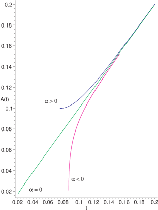
FIG. 1.: Plots from Eq. (19). We set $A(1)=1$, $kH_{o}^{2}=12$, and $\alpha H_{o}^{2}=(0;\,\pm 1.25\times 10^{-4})$ as illustrative values.

For the Euclidean section, by suitably choosing the origin of time, expression (19) can be solved as

$$A^{2}=H_{o}\,\sqrt{\frac{2}{3}\,(k\,c^{2}\,t^{2}+12\,\alpha)}.$$ (21)

¿From Eq. (17), the average strength of the magnetic field $H$ evolves in time as

$$H^{2}=\frac{3}{2}\,\frac{1}{{k\,c^{2}\,t^{2}}+12\,\alpha}.$$ (22)

Expression (21) is singular for $\alpha<0$, as there exist a time $t=\sqrt{-12\alpha/k\,c^{2}}$ for which $A(t)$ is arbitrarily small. Otherwise, for $\alpha>0$ we recognize that at $t=0$ the radius of the universe attains a minimum value $A_{min}$, which is given from

$$A^{2}_{min}=H_{o}\,\sqrt{8\,\alpha}.$$ (23)

Therefore, the actual value of $A_{min}$ depends on $H_{o}$, which turns out to be the unique free parameter of the present model. The energy density $\rho_{\gamma}$ given by Eq. (15) reaches its maximum value $\rho_{max}=1/64\alpha$ at the instant $t=t_{c}$, where

$$t_{c}=\frac{1}{c}\,\sqrt{\frac{12\,\alpha}{k}}.$$ (24)

For smaller values of $t$ the energy density decreases, vanishing at $t=0$, while the pressure becomes negative. Only for times $t\,\raisebox{-2.15277pt}{$\stackrel{{\scriptstyle<}}{{\sim}}$}\,10\sqrt{\alpha/kc^{2}}$ the nonlinear effects are relevant for cosmological solution of the normalized scale factor, as shown in Fig. 2. Indeed, solution (21) fits the standard expression (12) of the Maxwell case at the limit of large times.

                          

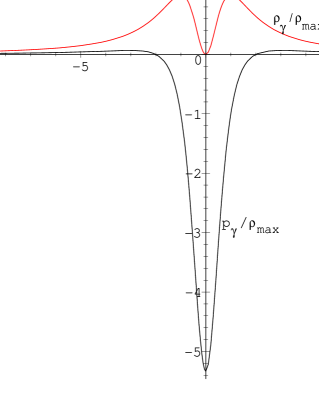
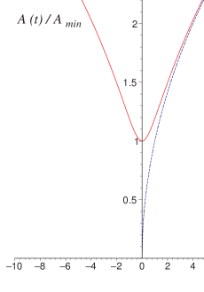
FIG. 2.: On the left panel: time dependence of the electromagnetic energy density $\rho_{\gamma}$ and pressure $p_{\gamma}$. $\rho_{max}=1/64\alpha$ and $t_{c}$ is given by Eq. (24). On the right panel: nonsingular behavior of the scale factor $A(t)$. $A_{min}$ and $t_{c}$ are given from Eqs. (23),(24). The corresponding classical expression (12) is shown (dashed line) for comparison, with $A_{o}=A_{min}$.

The energy-momentum tensor (14) is not trace-free for $\alpha\neq 0$. Thus, the equation of state $p_{\gamma}=p_{\gamma}(\rho_{\gamma})$ is no longer given by the Maxwellian value; it has instead a quintessential-like term [22] which is proportional to the constant $\alpha$. That is

$$p_{\gamma}=\frac{1}{3}\,\rho_{\gamma}-\frac{16}{3}\,\alpha\,H^{4}.$$ (25)

Equation (25) can also be written in the form

$$p_{\gamma} = \frac{1}{3}\,\rho_{\gamma}-\frac{1}{24\alpha}\left\{(1-32\alpha\rho_{\gamma})\right.$$ (27)

$$\left.+[1-2\Theta(t-t_{c})]\sqrt{1-64\alpha\rho_{\gamma}}\right\},$$

where $\Theta(z)$ it the Heaviside step function. The right-hand side of Eq. (27) behaves as $(1-64\alpha\rho_{\gamma})\rho_{\gamma}/3$ for $t>t_{c}$ in the Maxwell limit $\alpha\rho_{\gamma}\ll 1$.

The maximum of the temperature corresponding to $t=t_{c}$ is given by

$$T_{max}=\left(\frac{c}{24\alpha\sigma}\right)^{1/4},$$ (28)

where $\sigma$ is the Stefan-Boltzmann constant.

IV Conclusions

The consequences of the minimal coupling of gravity with second order nonlinear electrodynamics (13) were examined. ¿From the cosmological point of view, the proposed modification is relevant only in the primeval era of the universe. Indeed, the class of theories $\alpha>0$ leads to nonsingular solutions for which the scale factor $A(t)$ attains a minimum value. The regularity of the cosmological solution (21) is to be attributed to the fact that, for $t<\sqrt{24\alpha/kc^{2}}$, the quantity $\rho+3p$ becomes negative.

A Ultrarelativistic matter contribution

Beside photons there are plenty of other particles, and physics of the early universe deals with various sort of matter. In the standard framework they are treated in terms of a fluid with energy density $\rho_{\nu}$, which satisfies an ultrarelativistic equation of state $p_{\nu}=\rho_{\nu}/3$. Adding the contribution of this kind of matter to the average energy-momentum tensor of the photons it follows that $\rho_{\nu}=KA^{-\,4},$ where $K$ is an arbitrary positive constant. This result allows us to treat such extra matter as nothing but a reparametrization of the constants $H_{o}$ and $\alpha$ as $\hat{H}_{o}^{2}=H_{o}^{2}+2K$ and $\hat{\alpha}=\alpha{H_{o}^{4}}/{(H_{o}^{2}+2K)^{2}}$. The net effect of this is just to diminish the value of $A_{min}$ as

$$\hat{A}\mbox{}_{min}=\left(\frac{H_{o}^{2}}{H_{o}^{2}+2K}\right)^{1/4}A_{min}.$$ (A1)

Therefore, it turns out that the phenomenon of reversing the sign of the expansion factor $3\dot{A}/A$ due to the high negative pressure of the photons is not essentially modified by the ultrarelativistic gas. Only an exotic fluid possessing energy density $\rho_{exotic}\sim A^{n}$ with $n\leq-\,8$ could be able to modify the above result. However, this situation seems to be a very unrealistic case.

REFERENCES

- [1] E. W. Kolb and M. S. Turner, The Early Universe (Addison-Wesley, Redwood City, CA, 1990).
- [2] R. Brandenberger, in Proceedings of the VIII Brazilian School of Cosmology and Gravitation, edited by M. Novello (Editions Frontiéres, Singapore, 1996).
- [3] L. Kofman, A. Linde, and A. A. Starobinsky Phys. Rev. D 56, 3258 (1997).
- [4] W. de Sitter, Proc. K. Ned. Akad. Wet. 19, 1217 (1917).
- [5] M. Novello and J. M. Salim, Phys. Rev. D 20, 377 (1979); A. Saa, E. Gunzig, L. Brenig, V. Faraoni, T. M. Rocha Filho, and A. Figueiredo, gr-qc/0012105 (2000).
- [6] V. Mukhanov and R. Brandenberger, Phys. Rev. Lett. 68, 1969 (1992). See also R. Brandenberger, V. Mukhanov, and A. Sornborger, Phys. Rev. D 48, 1629 (1993); R. Moessner and M. Trodden, ibid 51, 2801 (1995).
- [7] M. Novello, L. A. R. Oliveira, J. M. Salim and E. Elbaz, Int. J. Mod. Phys. A 1, 641 (1993).
- [8] G. L. Murphy, Phys. Rev. D 8, 4231 (1973); J. M. Salim and H. P. de Olivera, Acta Phys. Pol. B 19, 649 (1988).
- [9] R. Garcia-Salcedo and N. Breton, Int. J. Mod. Phys. A 15 (27), 4341 (2000).
- [10] R. Klippert, V. A. De Lorenci, M. Novello, and J. M. Salim, Phys. Lett. B 472, 27 (2000); G. Veneziano, hep-th/0002094 2000.
- [11] S. W. Hawking and G. F. R. Ellis, The Large Scale Structure of Spacetime (Cambridge University Press, Cambridge, England, 1973); R. M. Wald, General Relativity (Univ. Chicago Press, Chicago, 1984).
- [12] M. Novello, in Proceedings of the II Brazilian School of Cosmology and Gravitation, edited by M. Novello (J. Sansom & Cia., Rio de Janeiro, 1980) (in Portuguese).
- [13] R. C. Tolman and P. Ehrenfest, Phys. Rev. 36, 1791 (1930); M. Hindmarsh and A. Everett, Phys. Rev. D 58, 103505 (1998).
- [14] H. P. Robertson, Rev. Mod. Phys. 5, 62 (1933); D. Edwards, Astrophys. Space Sci. 24, 563 (1973); R. Coqueraux and A. Grossmann, Ann. Phys. (N.Y.) 143, 296 (1982); M. Dabrowski and J. Stelmach, Astron. J. 92, 1272 (1986).
- [15] T. Tajima, S. Cable, K. Shibata, and R. M. Kulsrud, Astrophys. J. 390, 309 (1992); M. Giovannini and M. Shaposhnikov, Phys. Rev. D 57, 2186 (1998).
- [16] A. Campos and B. L. Hu, Phys. Rev. D 58, 125021 (1998).
- [17] G. Dunne and T. Hall, Phys. Rev. D 58, 105022 (1998); G. Dunne, Int. J. Mod. Phys. A 12, 1143 (1997).
- [18] M. Joyce and M. Shaposhnikov, Phys. Rev. Lett. 79, 1193 (1997).
- [19] C. Thompson and O. Blaes, Phys. Rev. D 57, 3219 (1998); K. Subramanian and J. D. Barrow, ibid 58, 883502 (1998).
- [20] K. Jedamzik, V. Jatalinić, and A. V. Olinto, Phys. Rev. D 57, 3264 (1998).
- [21] I. S. Gradshteyn and I. M. Ryzhik, Table of Integrals, Series, and Products, (Academic, London, 1965).
- [22] R. R. Caldwell, R. Dare, and P. J. Steinhardt, Phys. Rev. Lett. 80, 1582 (1998).