DFTT-32/98

gr-qc/9806073

Weighing the String Mass
with the COBE Data

M. Gasperini

Dipartimento di Fisica Teorica, Università di Torino,
Via P. Giuria 1, 10125 Turin, Italy
and

Istituto Nazionale di Fisica Nucleare, Sezione di Torino, Turin, Italy

In the context of the pre-big bang scenario the large-scale CMB anisotropy can be seeded by a primordial background of very light (or massless) axion fluctuations. In that case the slope of the temperature anisotropy spectrum, allowed by present observations, defines an allowed range of values for the string mass scale. Conversely, from the theoretical expected value of the string scale we can predict the slope of the anisotropy spectrum. In both cases there is a remarkable agreement between observations and theoretical expectations.

——————————

To appear in

Proc. of the Euroconference “Fifth Paris Cosmology Colloquium”
Observatoire de Paris, 3-5 June 1998 – Eds. H. J. De Vega and N. Sanchez

(World Scientific, Singapore)

1

WEIGHING THE STRING MASS WITH THE COBE DATA

MAURIZIO GASPERINI

Dipartimento di Fisica Teorica, Università di Torino,

Via P. Giuria 1, 10125, Turin, Italy

and Istituto Nazionale di Fisica Nucleare, Sezione di Torino, Turin, Italy

In the context of the pre-big bang scenario the large-scale CMB anisotropy can be seeded by a primordial background of very light (or massless) axion fluctuations. In that case the slope of the temperature anisotropy spectrum, allowed by present observations, defines an allowed range of values for the string mass scale. Conversely, from the theoretical expected value of the string scale we can predict the slope of the anisotropy spectrum. In both cases there is a remarkable agreement between observations and theoretical expectations.

Preprint No. DFTT-32/98;           E-print Archives: gr-qc/9806073

1 Introduction

The aim of this paper is to review, and briefly discuss, a possible mechanism for generating the large-scale CMB anisotropy, based on a primordial background of axion fluctuations acting as seeds for scalar metric perturbations^?,?,?.

Such a mechanism is particularly appropriate to pre-big bang models^? formulated in a string cosmology context, since in that case it seems difficult^? to generate the observed anisotropy through the standard inflationary mechanism. Let me explain why.

At very large angular scales, the temperature anisotropy spectrum is determined by the metric fluctuation spectrum $\Phi_{k}$ through the well-know Sachs-Wolfe (SW) effect^?:

$$\left(\Delta T\over T\right)_{k}\sim\Phi_{k}.$$ (1.1)

Metric fluctuations, directly amplified by the accelerated evolution of the background, have a spectrum that depends on the value of the Hubble scale at the time of horizon crossing,

$$\Phi_{k}\sim\left(H\over M_{p}\right)_{k}$$ (1.2)

($M_{p}$ is the Planck mass). In the standard de Sitter (or quasi-De Sitter) inflationary scenario $H$ is constant in time, so that the spectrum is scale invariant. A typical normalization of the spectrum, corresponding to inflation occurring roughly at the GUT scale,

$${H\over M_{p}}\sim{{\rm GUT~{}curvature~{}scale\over PLANCK~{}scale}}\sim 10^{-5},$$ (1.3)

is thus perfectly consistent with the anisotropy observed at the present horizon scale, $\Delta T/T\sim 10^{-5}$, and with the fact that the spectrum is scale-invariant.

Why this simple mechanism does not work in a string cosmology context? In string cosmology models the curvature scale grows with time, so that the spectrum of metric fluctuations (1.2) grows with frequency. In addition, the natural inflation scale corresponds to the string scale, so that the normalization of the spectrum, at the end-point frequency $k_{1}$, is controlled by the ratio

$$\left(H\over M_{p}\right)_{k_{1}}\sim{{\rm STRING~{}curvature~{}scale\over PLANCK~{}scale}}\sim 10^{-2}.$$ (1.4)

We are thus led to the situation qualitatively illustrated in Fig. 1. For pre-big bang models the slope of the spectrum is too steep, and the normalization too high, to be compatible with COBE observations^?. The slope is so steep, however, that the contribution of metric fluctuations to $\Delta T/T$ is certainly negligible at the COBE scale. So, on one hand there is no contradiction with observations, namely the COBE data cannot be used to rule out pre-big bang models. On the other hand, the problem remains: how to explain the observed anisotropy if the contribution of metric fluctuations is so small?

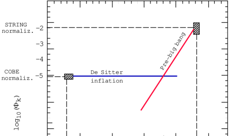
Figure 1: The contribution of primordial metric fluctuations to $\Delta T/T$, in the pre-big bang scenario, is expected to be negligible at the COBE scale.

A possible answer to this question comes from the observation that the previous argument applies to the primordial spectrum of metric fluctuations, directly amplified by the accelerated evolution of the background. There is an additional indirect contribution to the final metric perturbation spectrum, however, arising from the quantum fluctuations of other fields (let me call them, generically, $\sigma$), amplified during inflation. Even if such fluctuations are eventually negligible as sources of the metric background, $\rho_{\sigma}\ll\rho_{c}$, their inhomogeneous stress tensor generates metric fluctuations according to the standard gravitational equations, and they can act as “seeds” for temperature anisotropies through the SW effect, as before:

$${\rho_{\sigma}\over\rho_{c}}\sim\Phi\sim{\Delta T\over T}$$ (1.5)

Why the seed mechanism can work? First of all because, unlike metric perturbations, there are fields whose fluctuations can be amplified with a flat spectrum even in the context of the pre-big bang scenario.

Second because the contribution to $\Delta T/T$ is quadratic in the seed fields, and not linear like in case of metric perturbations. So, even if the amplitude of seed fluctuations is still normalized at the string curvature scale, the square of the amplitude is not very far from the expected value $10^{-5}$:

$${\Delta T\over T}\sim\Phi\sim\sigma^{2}\sim\left({\rm STRING~{}curvature~{}scale\over PLANCK~{}scale}\right)^{2}\sim 10^{-4}.$$ (1.6)

In addition, we must recall that the string normalization is imposed at the end-point of the spectrum^? (roughly, at the GHz scale), while COBE observations constrain the spectrum at the present horizon scale ($\sim 10^{-18}$Hz). A very small (blue) tilt of the seed field spectrum is thus enough to make compatible the COBE normalization and the string normalization, as illustrated in Fig. 2.

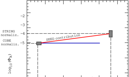
Figure 2: The amplitude of metric fluctuations induced by seeds may be consistent both with the COBE and the string normalization of the spectrum.

The basic question now becomes: are there fields, in the context of the pre-big bang scenario, whose fluctuations can be amplified with a flat enough spectrum, so as to seed metric fluctuations and to fit consistently the observed anisotropy?

In the following Sections I will present two possible examples that seem to be promising: the case of massless and massive axion fluctuations.

2 Massless axions as seeds of large-scale anisotropy

A first possible candidate for seeding the large-scale anisotropy is a stochastic background of massless pseudoscalar fluctuations^?. I will take, as a particular example, the so-called “universal” axion of string theory, namely the four-dimensional dual $\sigma$ of the Kalb-Ramond antisymmetric tensor $H_{\mu\nu\alpha}$, appearing in the low-energy string effective action:

$$S=-\int d^{4}x\sqrt{-g}e^{-\phi}\left[R+(\partial_{\mu}\phi)^{2}-{1\over 12}H_{\mu\nu\alpha}^{2}\right],$$

$$H^{\mu\nu\alpha}=e^{\phi}\epsilon^{\mu\nu\alpha\beta}\partial_{\beta}\sigma.$$ (2.1)

The whole discussion can be applied, however, to any type of pseudoscalar fluctuation amplified with a flat enough primordial energy spectrum.

I will concentrate my discussion on three points. First, I have to show that such axion fluctuations can be amplified with a final scale-invariant distribution of their spectral energy density $\Omega_{\sigma}$:

$$\Omega_{\sigma}(k,\eta)={d\rho_{\sigma}(k,\eta)\over\rho_{c}d\ln k}\sim{\rm scale~{}invariant}.$$ (2.2)

Second, I will show that the scalar metric fluctuation on a given scale $k$, at the time the scale re-enters the horizon, is precisely determined by the axion energy distribution evaluated at the conformal time of re-entry, $\eta_{re}\simeq k^{-1}$:

$$\Phi_{k}(\eta_{re})\sim\Omega_{\sigma}(k,\eta_{re}).$$ (2.3)

Third, I will show that the dominant contribution to the SW effect comes from a scale at the time it re-enters the horizon, so that the final temperature spectrum exactly reproduces the primordial seed spectrum:

$$\left(\Delta T\over T\right)_{k}\sim\Phi_{k}(\eta_{re})\sim\Omega_{\sigma}(k,\eta_{re}).$$ (2.4)

These last two results are far from being trivial, being a consequence of the particular time-dependence of the Bardeen spectrum induced by axion fluctuations (these results do not apply, for instance, to electromagnetic fluctuations^?). I will give in this paper only a sketch of the arguments leading to the above results. A detailed derivation can be found in Refs. [1,2].

1) The possibility of a flat axion spectrum^? can be easily checked by considering the axion perturbation equation written in terms of the canonical variable, $\psi=\sigma\xi$, and of the “pump” field $\xi=ae^{\phi/2}$ (here $\phi$ is the dilaton, and $a$ is the four-dimensional scale factor of the string frame metric). In the conformal time gauge one obtains from eq. (2.1) the effective action

$$S=\int d^{3}xd\eta~{}a^{2}e^{\phi}\left(\sigma^{\prime 2}+\sigma\nabla^{2}\sigma\right),$$ (2.5)

and the perturbation equation (for the Fourier modes $\psi_{k}$)

$$\psi_{k}^{\prime\prime}+\left[k^{2}-(\xi^{\prime\prime}/\xi)\right]\psi_{k}=0$$ (2.6)

(the prime denotes differentiation with respect to the conformal time $\eta$). Assuming, for instance, a power-law evolution of the pre-big bang background, $\xi\sim|\eta|^{\alpha}$, the perturbation equation reduces to a Bessel equation, and the normalized solution can be written in terms of the Hankel functions $H_{\nu}$ as

$$\psi_{k}=\eta^{1/2}H_{\nu}^{(2)}(k\eta),~{}~{}~{}~{}~{}~{}~{}~{}~{}~{}~{}~{}~{}~{}~{}~{}~{}\nu=|\alpha-1/2|,$$ (2.7)

where the Bessel index $\nu$ depends on the kinematic of the background. The spectral energy density, for modes re-entering in the radiation era, depends finally on the background as

$$\Omega_{\sigma}(k)\sim k^{3-2\nu}.$$ (2.8)

If we take now a very simple, higher-dimensional but isotropic vacuum solution of the string cosmology equations, in $d=3+n$ spatial dimensions^?,

$$a\sim|\eta|^{-1/(1+\sqrt{d})},~{}~{}~{}~{}~{}~{}~{}~{}~{}~{}~{}~{}~{}~{}~{}~{}~{}e^{\phi/2}\sim|\eta|^{-{3+\sqrt{d}\over 2(1+\sqrt{d})}},$$ (2.9)

we find that the spectral index depends on $d$,

$$3-2\nu={\sqrt{d}-3\over 1+\sqrt{d}},$$ (2.10)

and that the spectrum may be flat ($3-2\nu=0$), in particular^?, for $d=9$.

It is important to stress that a flat spectrum is possible, in the previous background, for axion fluctuations, but impossible for metric fluctuations which are characterized by a different pump field^?, $\xi=ae^{-\phi/2}$. With this pump field, in the same background (2.9), both the power $\alpha$ and the Bessel index $\nu$ are independent of $d$, and the spectrum is always growing with a cubic slope, in any number of dimensions:

$$\xi=ae^{-\phi/2}\sim|\eta|^{1/2},~{}~{}~{}~{}~{}~{}~{}~{}~{}~{}~{}~{}~{}~{}~{}~{}~{}~{}3-2\nu=3.$$ (2.11)

2) Let us now compute the spectrum of metric perturbations seeded by a flat, primordial distribution of axion fluctuations. Define, as usual, the power spectrum of the Bardeen potential, $P_{\Phi}(k)$, in terms of the Fourier transform of the two-point correlation function:

$$\int{d^{3}k\over(2\pi k)^{3}}e^{i{\bf k}\cdot({\bf x}-{\bf x^{\prime}})}P_{\Phi}(k)=\langle\Phi(x)\Phi(x^{\prime})\rangle$$ (2.12)

(the brackets denote spatial average, or expectation value if perturbations are quantized). The square root of the two-point function, evaluated at a comoving distance $k^{-1}$, represents the typical amplitude of fluctuations on a scale $k$:

$$\left(\langle\Phi(x)\Phi(x^{\prime})\rangle\right)^{1/2}_{|x-x^{\prime}|=k^{-1}}\sim k^{3/2}|\Phi_{k}|.$$ (2.13)

Define also the power spectrum of the seed stress tensor, in the same way (no sum over $\mu$, $\nu$):

$$\int{d^{3}k\over(2\pi k)^{3}}e^{i{\bf k}\cdot({\bf x}-{\bf x^{\prime}})}P_{\mu}^{\nu}(k)=\langle T_{\mu}^{\nu}(x)T_{\mu}^{\nu}(x^{\prime})\rangle-\langle T_{\mu}^{\nu}(x)\rangle^{2}.$$ (2.14)

Metric fluctuations and seed fluctuations are related by the cosmological perturbation equations. By taking into account the important contribution of the off-diagonal components of the axion stress tensor one finds, typically, that Bardeen spectrum and axion energy density spectrum are related by^?:

$$P_{\Phi}^{1/2}(k)\sim G\left(a\over k\right)^{2}P_{\rho}^{1/2}(k),$$ (2.15)

where

$$\int{d^{3}k\over(2\pi k)^{3}}e^{i{\bf k}\cdot({\bf x}-{\bf x^{\prime}})}P_{\rho}(k) = \langle\rho_{\sigma}(x)\rho_{\sigma}(x^{\prime})\rangle-\langle\rho_{\sigma}(x)\rangle^{2}$$ (2.16)

$$\sim \langle\sigma^{\prime 2}(x)\sigma^{\prime 2}(x^{\prime})\rangle-\langle\sigma^{\prime 2}(x)\rangle^{2}+...$$

It may be interesting to note that the two-point correlation function of the energy density becomes a four-point function of the seed field, since the energy is quadratic in the axion field.

Using the condition of stochastic average for the axion field^?,

$$=\langle\sigma^{\prime}({\bf k},\eta)\sigma^{\prime\ast}({\bf k^{\prime}},\eta)\rangle=(2\pi)^{3}\delta^{3}(k-k^{\prime})\Sigma({\bf k},\eta),$$ (2.17)

we find that the energy density spectrum reduces to a convolution of Fourier transforms,

$$P_{\rho}(k)\sim{k^{3}\over a^{4}}\int d^{3}p~{}\Sigma(p)\Sigma(|k-p|)+...~{}~{},$$ (2.18)

which is dominated by the region $p\eta\sim 1$ for a flat enough axion spectrum^?,?. By expressing the convolution through the spectral energy density $\Omega_{\sigma}$, and evaluating the Bardeen potential at the time of re-entry $\eta_{re}\sim k^{-1}$, we are led finally to relate the Bardeen spectrum and the axion spectrum as

$$P_{\Phi}^{1/2}(k,\eta_{re})\sim k^{3/2}\left|\Phi_{k}(\eta_{re}\right|\sim\Omega_{\sigma}(k,\eta_{re}).$$ (2.19)

In the next (and last) step of my discussion I will explain why we are interested in metric fluctuations evaluated at the time of re-entry.

3) Let us come back, finally, to the seed contribution to $\Delta T/T$. In the multipole expansion of the temperature anisotropies,

$$\left\langle{\delta T\over T}({\bf n}){\delta T\over T}({\bf n}^{\prime})\right\rangle_{{~{}}_{\!\!({\bf n\cdot n}^{\prime}=\cos\vartheta)}}~{}~{}=~{}~{}~{}~{}{1\over 4\pi}\sum_{\ell}(2\ell+1)C_{\ell}P_{\ell}(\cos\vartheta)~{},$$ (2.20)

the coefficients $C_{\ell}$, at very large angular scales ($\ell\ll 100$), are determined by the SW effect as follows^?,?:

$$C_{\ell}^{SW}={2\over\pi}\int d~{}(\ln k)\left\langle\left[\int^{k\eta_{0}}_{k\eta_{dec}}d(k\eta)~{}k^{3/2}(\Psi-\Phi)({\bf k},\eta)j_{\ell}^{\prime}\left(k\eta_{0}-k\eta\right)\right]^{2}\right\rangle.$$ (2.21)

Here $\Phi$ and $\Psi$ are the two-independent components of the gauge-invariant Bardeen potential, and $j_{\ell}$ are the spherical Bessel functions. Eq. (2.21) takes into account both the “ordinary” and the “integrated” SW contribution, namely the complete distortion of the geodesics of the CMB photons (due to shifts in the gravitational potential), from the time of decoupling $\eta_{dec}$ down to the present time $\eta_{0}$. By inserting the Bardeen potential determined by the axion field, one now finds that the time integral is dominated by the region $k\eta\sim 1$. Using eq. (2.19) we obtain

$$C_{\ell}^{SW} \sim \int d(\ln k)~{}k^{3/2}|\Phi_{k}(\eta_{re})|^{2}j_{\ell}(k\eta_{0})|^{2}$$ (2.22)

$$\sim \int d(\ln k)~{}\Omega_{\sigma}^{2}(k,\eta_{re})$$

($j_{\ell}$ are the spherical Bessel functions). Here is why it was important to evaluate the Bardeen spectrum at the time of re-entry, $\eta_{re}\sim k^{-1}$.

From the final expression that gives the multipole coefficients in terms of the axion spectral distribution^?,? we can extract, in particular, the value of the quadrupole coefficient $C_{2}$:

$$C_{2}\simeq\Omega_{\sigma}^{2}(k_{0},\eta_{0})\simeq\left(M_{s}\over M_{p}\right)^{4}\left(k_{0}\over k_{1}\right)^{n-1},$$ (2.23)

where $n$ is the spectral index (sufficiently near to $1$) characterizing the primordial axion distribution, $k_{0}$ is the comoving scale of the present horizon, and $k_{1}$ the end-point of the spectrum, namely the maximal amplified comoving frequency.

The peak amplitude of the axion spectrum, at the end-point frequency, is controlled by the fundamental ratio between string and Planck mass, $M_{s}/M_{p}$. The quadrupole coefficient, on the other hand, is presently determined by COBE as^?

$$C_{2}=(1.9\pm 0.23)\times 10^{-10}.$$ (2.24)

This experimental value, inserted into eq. (2.23), implies a relation between the string mass and the spectral index of the temperature anisotropy, which is illustrated in Fig. 3.

Figure 3: Relation between string mass and spectral index of CMB anisotropy, obtained by combining the COBE normalization of the spectrum with the prediction of an axionic seed model of the anisotropy. The dashed lines correspond to the experimentally allowed range of the spectral index. The shaded area corresponds to the theoretically expected value of the string scale.

The experimentally allowed range of the spectral index^? is, at present,

$$1\leq n\leq 1.4$$ (2.25)

(I have excluded the allowed values $0.8\leq n\leq 1$, which would imply in our case an over-critical axion production). It is remarkable that the corresponding allowed range of the string mass is perfectly compatible with theoretical expectations^?,

$$0.01~{}\raise 1.72218pt\hbox{$<$}\kern-8.00003pt\lower 2.6694pt\hbox{$\sim$}~{}M_{s}/M_{p}~{}\raise 1.72218pt\hbox{$<$}\kern-8.00003pt\lower 2.6694pt\hbox{$\sim$}~{}0.1$$ (2.26)

(see Fig. 3). Conversely, the above expected range for $M_{s}$ implies a spectral index around $1.1$ or $1.2$ (see again Fig. 3), which is also in very good agreement with observations.

It must be stressed, however, that eq. (2.23) is valid in the assumption that the inflation scale of pre-big bang models exactly coincides with the string mass scale. If the two scales were slightly different, an additional source of uncertainty would be introduced into the relation (2.23).

3 Massive axions as seeds of large-scale anisotropy

Up to now the discussion was devoted to massless pseudoscalar perturbations. It is likely, however, that axions become massive in the post-inflationary era: it is thus important to consider this possibility also.

Let me say immediately that also in the massive case the seed mechanism can work^?, and let me introduce the main differences between the massless and the massive case.

A first difference is the relation between the Bardeen potential $\Phi$ and the axion energy density $\rho_{\sigma}$. In the massless case the perturbation equations, taking into account the important contribution of all the off-diagonal terms of the axion stress tensor, lead to^?

$$\Phi_{k}\sim G\left(a\over k\right)^{2}\rho_{\sigma}(k).$$ (3.1)

In the massive case, on the contrary, the axion stress tensor can be approximated as a diagonal, perfect fluid stress tensor, and we obtain^?

$$\Phi_{k}\sim Ga^{2}\eta^{2}\rho_{\sigma}(k).$$ (3.2)

Also, in the massless case the convolution (2.18) for the axion energy density is dominated by the region^?,? $p\sim\eta^{-1}$, while in the massive case by^?,? $p\sim k$. In the massless case the integrated SW effect is the dominant one^?, while in the massive case the ordinary SW effect is dominant^?.

In spite of all these differences, the final result is similar, and in both cases the quadrupole coefficient is determined by the axion spectral energy density as

$$C_{2}\sim\Omega_{\sigma}^{2}(k_{0},\eta_{0}).$$ (3.3)

In the massive case, however, the axion spectrum is affected by non-relativistic corrections. In order to include such corrections, it is convenient^? to distinguish between modes that become non-relativistic ($k/a<m$) when they are already inside the horizon ($k/a>H$), and modes that become non-relativistic when they are still outside the horizon ($k/a<H$). In the first case the energy density is simply rescaled by the factor $m/\omega$ (where $\omega=k/a$ is the proper frequency), and the spectrum looses a power,

$$\Omega_{\sigma}\sim\omega^{3-2\nu}\rightarrow\left(m\over\omega\right)\Omega_{\sigma}\sim\omega^{2-2\nu}.$$ (3.4)

In the second case, on the contrary, the spectral slope is the same as the relativistic one, because of the freezing of perturbations outside the horizon. The difference between the two regimes is graphically illustrated in Fig. 4, where $\omega_{m}$ represents the limiting frequency of a mode that becomes non-relativistic just at the moment of horizon crossing.

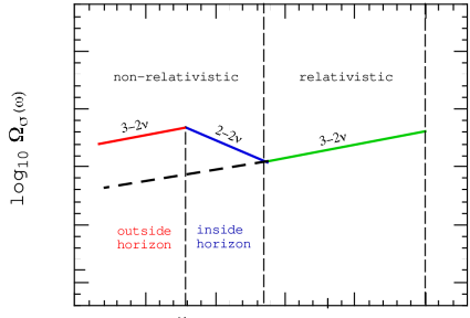
Figure 4: Mass-dependent enhancement of the spectrum at low frequency, due to non-relativistic corrections. The non-relativistic part of the spectrum, to the left of $\omega=m$, has a peak in correspondence of the frequency mode $\omega_{m}$ that becomes non-relativistic at the time it re-enters the horizon.

As clearly shown in Fig. 4, the effect of non-relativistic corrections is to enhance the amplitude of the spectrum at low frequency. The enhancement is proportional to the square root of the axion mass if, at the time when axions become massive, the scale $\omega_{m}$ is still outside the horizon. In the opposite case the enhancement is linear in the axion mass. An explicit calculation, for a class of cosmological models that remain radiation-dominated from the end of inflation down to the equilibrium epoch, leads in fact to the following expression for the low-frequency branch of the spectrum^?:

$$\Omega_{\sigma} = \left(M_{s}\over M_{p}\right)^{2}\left(m\over H_{eq}\right)^{1/2}\left(\omega\over\omega_{1}\right)^{3-2\nu},~{}~{}~{}~{}~{}~{}~{}~{}~{}~{}~{}~{}\left(m\over H_{eq}\right)^{1/2}<{T_{m}\over{\rm eV}},$$ (3.5)

$$= \left(M_{s}\over M_{p}\right)^{2}\left(m\over H_{eq}\right)\left({\rm eV}\over T_{m}\right)\left(\omega\over\omega_{1}\right)^{3-2\nu},~{}~{}~{}~{}~{}~{}\left(m\over H_{eq}\right)^{1/2}>{T_{m}\over{\rm eV}}.$$

Here $H_{eq}\sim 10^{-27}$ eV is the Hubble scale at the time of matter-radiation equilibrium, and $T_{m}$ is the temperature scale of mass generation (for instance, $T_{m}\sim 100$ MeV if axions become massive at the epoch of chiral symmetry breaking). In both cases the slope is the same as that of the massless spectrum, $3-2\nu$.

The amplitude of the spectrum now depends on the axion mass, and the constraint imposed by the COBE normalization (2.24) necessarily bounds the allowed range of masses. This might represent a problem, in general: since the slope cannot be too steep at low frequency (according to eq. (2.25)), the allowed mass could be too low to be compatible with realistic axion models.

This conclusion, based on the effect illustrated in Fig. 4, refers however to a relativistic spectrum characterized by a constant slope. On the other hand, it is quite easy to imagine, and to implement in practice, a model of background in which the relativistic axion spectrum is flat enough at low frequency (as required by a fit of the large-scale anisotropy), and much steeper at high frequency. A simple example is illustrated in Fig. 5, where I have compared two spectra. The first one is flat everywhere, except for non-relativistic corrections. The second one is flat at low frequency, and steeper at high frequency. It is evident that the steeper and the longer the high-frequency branch of the spectrum, the larger is the suppression of the amplitude at low frequency, and the larger is the axion mass allowed by the COBE normalization at $\omega=\omega_{0}$.

Figure 5: Two examples of axion spectra with non-relativistic corrections. Note the common normalization at the end-point frequency $\omega_{1}$, in spite of the different slopes in the different frequency regimes.

We have analysed this possibility^? in an explicit two-parameter model of background, including exact solutions of the low-energy string cosmology equations with classical string sources. The allowed region in parameter space turns out to be consistent with a very wide range of axion masses, from the equilibrium scale $m\sim 10^{-27}$ eV up to $m\sim 100$ MeV (higher masses are not acceptable, because of the axion decay into photons). We can say, therefore, that there is no fundamental incompatibility between a fit of the large-scale anisotropy, and an axion mass in the expected range of conventional axion models.

4 Conclusion

A stochastic cosmic background of pseudoscalar fluctuations, produced with a flat enough primordial spectrum, can seed the observed CMB anisotropy at very large angular scales. The end-point normalization of the spectrum imposed by the string cosmology scenario, and the observational normalization at the COBE scale, are consistent both for massless and massive fluctuations.

In spite of these promising results, it should be clearly stressed that this approach to CMB anisotropy is only the first step of a much longer research program, still to be implemented. Many important questions are still waiting for an answer, among which the crucial one, in my opinion, concerns the possible differences at smaller angular scales between this mechanism and the standard inflationary mechanism of anisotropy production. In particular: is the statistic non-Gaussian? are there shifts in the position of the Doppler peak? etc …

The answer to these questions is at present unclear, but we hope to provide answers in future papers.

Acknowledgments: I am very grateful to Ruth Durrer, Mairi Sakellariadou and Gabriele Veneziano for a fruitful collaboration which led to the results reported in this paper. I wish to thank also the Hector De Vega and Norma Sanchez for their kind invitation, and for the perfect organization of this interesting Euroconference.

References

- [1] R. Durrer, M. Gasperini, M. Sakellariadou and G. Veneziano, Seeds of large-scale anisotropy in string cosmology, gr-qc/9804076.
- [2] R. Durrer, M. Gasperini, M. Sakellariadou and G. Veneziano, Massless (pseudo)scalar seeds of CMB anisotropy, astro-ph/9806015.
- [3] M. Gasperini and G. Veneziano, Constraints on pre-big bang models for seeding large-scale anisotropy by massive Kalb–Ramond axions, hep-ph/9806327.
- [4] M. Gasperini and G. Veneziano, Astropart. Phys. 1, 317 (1993); Mod. Phys. Lett. A 8, 3701 (1993); Phys. Rev. D 50, 2519 (1994). An updated collection of papers on the pre-big bang scenario is available at http://www.to.infn.it/~gasperin/.
- [5] R. Brustein, M. Gasperini, M. Giovannini, V. F. Mukhanov and G. Veneziano, Phys. Rev. D 51, 6744 (1995).
- [6] R. K. Sachs and A. M. Wolfe. Ap. J. 147, 73 (1967).
- [7] G. F. Smoot et al., Ap. J. 396, L1 (1992); C. L. Bennett et al., Ap. J. 430, 423 (1994).
- [8] R. Brustein, M. Gasperini, and G. Veneziano, Phys. Rev. D 55, 3882 (1997).
- [9] E. J. Copeland, R. Easther and D. Wands, Phys. Rev. D 56, 874 (1997); E. J. Copeland, J. E. Lidsey and D. Wands, Nuc. Phys. B 506, 407 (1997).
- [10] G. Veneziano, Phys. Lett. B 265, 287 (1991).
- [11] A. Buonanno, K. A. Meissner, C. Ungarelli and G. Veneziano, JHEP01, 004 (1998).
- [12] M. Gasperini and M. Giovannini, Phys. Rev. D 47, 1519 (1993).
- [13] R. Durrer, Phys. Rev. D 42, 2533 (1990); Fund. of Cosmic Physics 15, 209 (1994).
- [14] A. J. Banday et al., Astrophys. J. 475, 393 (1997).
- [15] G.F. Smoot and D. Scott, in L. Montanet et al., Phys. Rev. D 50, 1173 (1994) (1996 update).
- [16] V. Kaplunowski, Phys. Rev. Lett. 55, 1036 (1985).