Scale invariance and critical gravitational collapse

Abstract

We examine ways to write the Choptuik critical solution as the evolution of scale invariant variables. It is shown that a system of scale invariant variables proposed by one of the authors[1] does not evolve periodically in the Choptuik critical solution. We find a different system, based on maximal slicing. This system does evolve periodically, and may generalize to the case of axisymmetry or of no symmetry at all.

I Introduction

Scaling behavior, as first found by Choptuik[2], occurs at and near the threshold of black hole formation in the gravitational collapse of many types of matter[3, 4, 5, 6, 7, 8, 9, 10]. For a one parameter family of initial data slightly above the threshold, the mass of the black hole scales like ${{(p-p*)}^{\gamma}}$. Here $p$ is the parameter, $p*$ is its critical value and $\gamma$ is a constant that depends on the type of matter, but not on the family of data. For initial data slightly below the threshold, the maximum curvature scales like ${{({p*}-p)}^{-2\gamma}}$ where $\gamma$ is the same constant as in the black hole mass scaling law.[11] For some types of matter, the critical solution ($p=p*$) has periodic self-similarity: after a certain amount of time, the metric and matter variables repeat themselves with the scale of space shrunk. For other types of matter, the critical solution has exact self-similarity: only the overall spatial scale changes with time.

Most of the work done on scaling has assumed spherical symmetry. However, Abrahams and Evans have found scaling in the collapse of axisymmetric gravity waves[6]. In addition, perturbative work of Gundlach on fluid collapse assumes no symmetries at all.[12] Thus (for certain types of matter) scaling seems to be a generic property of critical gravitational collapse.

The scaling of black hole mass (and of maximum curvature) has been explained[13, 14, 15] subject to the following assumptions: (i) the critical solution is periodically self-similar or exactly self-similar and (ii) the critical solution has exactly one unstable mode. What remains to be explained is why the critical solution is periodically self-similar (or exactly self-similar). It has been noted[1, 13, 14] that the property of periodic self-similarity bears a striking resemblance to periodicity of a limit cycle of a dynamical system. Correspondingly, exact self-similarity of a critical solution resembles a limit point of a dynamical system. Furthermore, one can turn “resembles” to “is” by writing the Einstein field equations as a dynamical system of scale invariant variables.

To write Einstein’s equations as a dynamical system requires a choice of foliation (time slicing) for the spacetime. Some foliations will be compatible with the periodic self-similarity and some will not. More precisely, periodic self-similarity means that there is a diffeomorphism $\zeta$ and a number $\Delta$ such that ${\zeta^{*}}\left({g_{ab}}\right)={e^{-2\Delta}}\,{g_{ab}}$. A foliation is a one parameter family of spacelike (or null) hypersurfaces $\Sigma(t)$. For a periodically self-similar spacetime, call a foliation compatible provided that for each $t_{0}$ there is a $t_{1}$ such that $\zeta\left(\Sigma(t_{0})\right)=\Sigma({t_{1}})$. In more physical terms a foliation is compatible if for each slice, there is a later slice that is identical except for an overall change in the scale of space. For a given periodically self-similar spacetime, there are many foliations that are compatible. Simply choose any initial hypersurface $\Sigma({t_{0}})$. Carry it forward by the diffeomorphism $\zeta$ to form the hypersurface $\Sigma({t_{1}})$. For ${t_{0}}<t<{t_{1}}$, interpolate the hypersurfaces in any smooth way. Then extend that family to the whole spacetime using $\zeta$ and $\zeta^{-1}$. There are also many foliations that are not compatible. Thus compatibility is a property of the entire foliation, or equivalently of the prescription for the lapse. Given any initial slice, there is some compatible foliation that contains that slice. A dynamical systems explanation of Choptuik scaling requires a compatible foliation.

Note that compatibility is a condition on the lapse and is independent of the choice of shift. However, one may want to choose the evolution vector field so that the diffeomorphism $\zeta$ has the form $t\to t+\Delta$ with the spatial coordinates unchanged. This requires both a compatible foliation and a condition on the shift.

Most of the work done on Choptuik scaling has assumed spherical symmetry. Here the metric can be put in the form[2]

$$d{s^{2}}=-\,{\alpha^{2}}\,d{t^{2}}\;+\;{a^{2}}\,d{r^{2}}\;+\;{r^{2}}\,d{\Omega^{2}}\;\;\;.$$

Here $\alpha$ and $a$ are functions of $r$ and $t$; $d{\Omega^{2}}$ is the unit two-sphere metric and $r$ is the usual area coordinate. The surfaces of constant $t$ are orthogonal to the surfaces of constant $r$. Usually the condition $\alpha=1$ at $r=0$ is imposed so $t$ is proper time at the position of the central observer. This foliation is compatible.

A spherically symmetric metric can also be put in the form[16]

$$d{s^{2}}=-\,g\,du\,({\bar{g}}\,du\,+\,2\,dr)\;+\;{r^{2}}\,d{\Omega^{2}}\;\;\;.$$

Here $r$ and $d{\Omega^{2}}$ are as in equation (1) and $g$ and $\bar{g}$ are functions of $r$ and $u$. The “time” coordinate $u$ is constant along outgoing light rays and equal to proper time at the position of the central observer. This foliation is compatible.

A metric or matter variable is scale invariant provided that it is unchanged when ${g_{ab}}\to k\,{g_{ab}}$ for any positive constant $k$. The quantities $\alpha$ and $a$ in equation (1) are scale invariant: under a scale transformation, $\alpha$ and $a$ have the same form with only the overall scale of $r$ and $t$ changed. Similarly, the quantities $g$ and $\bar{g}$ in equation (2) are scale invariant. In spherical symmetry, the metric is determined by the matter. The type of matter treated by Choptuik[2] is a massless, minimally coupled scalar field $\phi$. Initial data for this system consists of the field and its normal derivative at a moment of time. The matter variables used in[2] are $(r/a)\,\partial\phi/\partial r$ and $(r/\alpha)\,\partial\phi/\partial t$. These variables are scale invariant. For the same physical system, in the coordinates of equation (2) the usual matter variable is $h\equiv\partial(r\phi)/\partial r$, which is scale invariant. Scale invariant variables have also been found for other types of matter.[17, 18]

While compatible foliations are known in the spherically symmetric case, Choptuik scaling is a generic phenomenon that does not seem to depend on symmetry. Therefore, one would like to find a compatible foliation for the general case. The foliations of equations (1) and (2) depend, in an essential way, on spherical symmetry. The constant $t$ slices of equation (1) are defined as orthogonal to the spherical area coordinate $r$. The constant $u$ slices of equation (2) are the null cones of the observer left invariant by the spherical symmetry. Thus, there does not seem to be any natural way to generalize these foliations to the case of axisymmetry or of no symmetry.

Thus, what should be done is to use a slicing condition that makes no reference to symmetry, find a set of scale invariant variables associated with that foliation, and check that the foliation is compatible. In practice, one can check compatibility on a case by case basis. That is, given a particular critical solution, say as the output of a numerical code, one can check numerically whether a particular foliation is compatible. In this paper, we will explicitly check compatibility only with the Choptuik critical solution: that is, the case of a spherically symmetric, minimally coupled scalar field.

In reference[1] a slicing condition was proposed that makes no reference to symmetry, and a set of scale invariant metric and matter variables associated with this foliation was found. However, it was not known whether this foliation was compatible. This paper provides an answer to that question. In section 2 we present the numerical methods used in this study and consider the foliation of reference[1]. We show that this foliation is not compatible with the Choptuik critical solution. In section 3 we find a different system of scale invariant variables based on maximal slicing, and show that maximal slicing is compatible with the Choptuik critical solution. We then consider the question of whether maximal slicing is compatible in the case of axisymmetry or no symmetry.

II Numerical Methods

Typically, in numerical relativity, one thinks of the slicing condition as a part of the numerical code that evolves the metric variables to find the spacetime. Thus, the prospect of analyzing the Choptuik critical solution using several different slicing conditions seems daunting. A numerical treatment of the Choptuik critical solution requires great accuracy and stability and a large range of spatial scales. It would be difficult to write a code that does these things well in an arbitrary slicing. Fortunately, this is not necessary. Given the data from a code that uses one slicing condition, one can produce numerically the foliations of other slicing conditions.

We begin with numerical data for the metric and scalar field for the Choptuik critical solution in the coordinates of equation (2), as found in reference[5] (using methods based on the work of Christodoulou[16] and of Goldwirth and Piran[19]). A spherically symmetric slice in these coordinates is given by $u=u(r)$. To produce a slice in these coordinates, we must express the slicing condition as a differential equation for $u(r)$ and then numerically solve that equation. For the $t=const.$ slices of equation (1), ${\nabla_{a}}t$ is orthogonal to ${\nabla_{a}}r$. Therefore these slices are given by

$${{du}\over{dr}}=-\;{1\over{\bar{g}}}\;\;\;.$$

To solve this equation numerically, for each $u$ we begin at $r=0$ and integrate outward using a Runge-Kutta method. For each $(r,u)$ value we find the value of $\bar{g}$ by interpolation using the values that we have from the output of the numerical code of reference[5].

Now suppose that we wish to find the maximal slices. For a surface $u=u(r)$, the extrinsic curvature is

$$K={W\over{2g}}\;{{\partial g}\over{\partial u}}\;+\;{g\over 2}\;{W^{3}}\;{{\partial{\bar{g}}}\over{\partial u}}\;+\;\left({1\over{gW}}\;-\;{\bar{g}}\,W\right)\;\left({1\over{4g}}\;{{\partial g}\over{\partial r}}\;+\;{1\over r}\right)$$

$$-\;{1\over 4}\;\left(g\,{\bar{g}}\,{W^{3}}\,+\,3\,W\right)\;{{\partial{\bar{g}}}\over{\partial r}}\;-\;{{g\,{W^{3}}}\over{{(du/dr)}^{3}}}\;{{{d^{2}}u}\over{d{r^{2}}}}$$

Where $W$ is given by

$$W\equiv{{\left[-\,g\,\left({\bar{g}}\,+\,2{{[du/dr]}^{-1}}\right)\right]}^{-1/2}}\;\;\;.$$

Thus the equation $K=0$ becomes

$${{{d^{2}}u}\over{d{r^{2}}}}={1\over g}\;{{\left({1\over W}\;{{du}\over{dr}}\right)}^{3}}\;\bigg{[}{W\over{2g}}\;{{\partial g}\over{\partial u}}\;+\;{g\over 2}\;{W^{3}}\;{{\partial{\bar{g}}}\over{\partial u}}\;+\;\left({1\over{gW}}\;-\;{\bar{g}}\,W\right)\;\left({1\over{4g}}\;{{\partial g}\over{\partial r}}\;+\;{1\over r}\right)$$

$$-\;{1\over 4}\;\left(g\,{\bar{g}}\,{W^{3}}\,+\,3\,W\right)\;{{\partial{\bar{g}}}\over{\partial r}}\bigg{]}\;\;\;.$$

For each $u$ we begin at $r=0$ and produce each surface by a Runge-Kutta integration outward using equation (6). Again, for each $(r,u)$ value, the quantities $g,{\bar{g}}$ and their derivatives are interpolated from the gridpoint values of these quantities.

Now suppose that our slicing condition involves a dynamical evolution of the lapse. Given the lapse $N$, we evolve the slice, and given the conditions on the slice, we evolve the lapse. For a slice, $u=u(r)$, the unit normal vector is

$${n^{a}}=W\;{{\left({\partial\over{\partial u}}\right)}^{a}}\;-\;W\;\left[{\bar{g}}\;+\;{1\over{du/dr}}\right]\;{{\left({\partial\over{\partial r}}\right)}^{a}}\;\;\;.$$

Since we wish only to know how the slices evolve, we can without loss of generality choose the shift to vanish. The coordinates of the slice then evolve by

$${\dot{u}}=N\,W\;\;\;,$$

$${\dot{r}}=-\,NW\;\left[{\bar{g}}\;+\;{1\over{du/dr}}\right]\;\;\;.$$

Here an overdot denotes derivative with respect to the evolution vector field $N\,{n^{a}}$.

For the system of reference[1] The lapse evolves by

$${\dot{N}}={1\over 3}\;{N^{2}}\,K\;\;\;.$$

Let $({h_{ab}},\,{K_{ab}},\,{D_{a}})$ be respectively the intrinsic metric, extrinsic curvature and derivative operator of a slice. The scale invariant metric variables associated with this foliation are ${{\tilde{h}}_{ab}}\equiv{N^{-2}}\,{h_{ab}},\,{{\tilde{K}}_{ab}}\equiv{N^{-1}}\,\left({K_{ab}}\,-\,[K/3]\,{h_{ab}}\right)$ and ${\omega_{a}}\equiv{N^{-1}}\,{D_{a}}N$.

We choose as the initial slice, a $t=const.$ slice generated using equation (3). The initial lapse is chosen to be $1$. The slice and lapse are then evolved using equations (8a), (8b) and (9) to produce a foliation of the spacetime.

We would now like to know whether this foliation is compatible. In a compatible foliation, the scale invariant variables repeat their behavior. Thus at corresponding slices, the scalar field $\phi$ as a function of $r/{\sqrt{N}}$ should be the same. To identify which slices are “corresponding,” define $\phi_{0}$ to be the value of $\phi$ at $r=0$. Then $\phi_{0}$ repeats itself and the slices that contain repeating values of $\phi_{0}$ are corresponding slices.

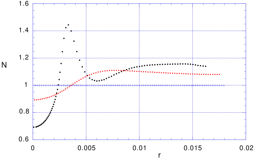
FIG. 1.: The lapse is plotted at the initial time and two later times. Note the steep peak in the lapse at the latest of these times.

Note from equation (9) that positive $K$ leads to an increasing lapse and, in fact, can cause the lapse to blow up in finite time. Figure 1 shows the lapse on three different slices. Note the steep peak in the lapse at the latest of these times. Shortly after this time, the lapse blows up. In the sequence of slices from the begining to the blow up of the lapse, $\phi_{0}$ does not even go through one cycle. Thus this foliation does not even exist long enough for a comparison of corresponding slices to take place. Therefore this foliation is not compatible.

III Maximal Slicing

A dynamical systems explanation of Choptuik scaling requires a compatible foliation and a set of scale invariant variables. For the Einstein-scalar equations, initial data on a slice $\Sigma$ are $({h_{ab}},\,{K_{ab}},\phi,\,P)$ where $h_{ab}$ is the intrinsic metric, $K_{ab}$ is the extrinsic curvature, $\phi$ is the scalar field and $P$ is its normal derivative. (recall that for $n_{a}$ the unit one-form normal to $\Sigma$ we have ${h_{ab}}={g_{ab}}+{n_{a}}{n_{b}},\;{K_{ab}}={{h_{a}}^{c}}{\nabla_{c}}{n_{b}}$ and $P={n^{a}}{\nabla_{a}}\phi$). If $({g_{ab}},\,\phi)$ is a solution of the Einstein-scalar equations and $c$ is any positive constant, then $({c^{2}}{g_{ab}},\,\phi)$ is also a solution. In this new solution, the unit normal one-form is now $c{n_{a}}$. It then follows that the initial data for this solution are $({c^{2}}{h_{ab}},\,c{K_{ab}},\,\phi,\,P/c)$. Since a maximal slice in $g_{ab}$ is also a maximal slice in ${c^{2}}{g_{ab}}$, it is natural to define the following equivalence relation among maximal initial data sets: a set $({{\tilde{h}}_{ab}},\,{{\tilde{K}}_{ab}},\,{\tilde{\phi}},\,{\tilde{P}})$ is equivalent to a set $({h_{ab}},\,{K_{ab}},\phi,\,P)$ provided that there is a positive constant $c$ such that

$$({{\tilde{h}}_{ab}},\,{{\tilde{K}}_{ab}},\,{\tilde{\phi}},\,{\tilde{P}})=({c^{2}}{h_{ab}},\,c{K_{ab}},\,\phi,\,P/c)\;\;\;.$$

Our set of scale invariant variables is an equivalence class of initial data. Is this set complete? That is, does an equivalence class of initial data contain enough information to determine its evolution? The answer is yes: simply take a member of the equivalence class, evolve it, and on each slice take its equivalence class. It does not matter which member of the equivalence class we pick, since in each case the metric that we produce differs only by an overall constant, leading to the same maximal slices and the same equivalence classes.

For the case of vacuum spacetimes, the scale invariant variables are simply equivalence classes of $({h_{ab}},\,{K_{ab}})$. For types of matter other than the scalar field, one must add scale invariant variables corresponding to initial data for the matter fields.

An equivalence class is a somewhat abstract variable. Is there a way to make these scale invariant variables more concrete? In some cases, the answer is yes. Suppose that ${K^{ab}}{K_{ab}}$ is bounded on a slice $\Sigma$ (as will be the case if $\Sigma$ is asymptotically flat) and define $\lambda\equiv{\sup_{\Sigma}}{{\left({K^{ab}}{K_{ab}}\right)}^{1/2}}$. Then under the transformation ${g_{ab}}\to{c^{2}}\,{g_{ab}}$ we have $\lambda\to\lambda/c$. Now define

$$({{\bar{h}}_{ab}},\,{{\bar{K}}_{ab}},\,{\bar{\phi}},\,{\bar{P}})\equiv({\lambda^{2}}\,{h_{ab}},\,\lambda\,{K_{ab}},\,\phi,\,P/\lambda)\;\;\;.$$

Then under ${g_{ab}}\to{c^{2}}\,{g_{ab}}$ the set $({{\bar{h}}_{ab}},\,{{\bar{K}}_{ab}},\,{\bar{\phi}},\,{\bar{P}})$ remains unchanged. In fact, this set is isomorphic to equivalence classes of $({h_{ab}},\,{K_{ab}},\,\phi,\,P)$. Thus for concreteness, in the case where ${K^{ab}}\,{K_{ab}}$ is bounded on each slice, we can use $({{\bar{h}}_{ab}},\,{{\bar{K}}_{ab}},\,{\bar{\phi}},\,{\bar{P}})$ as our set of scale invariant variables.

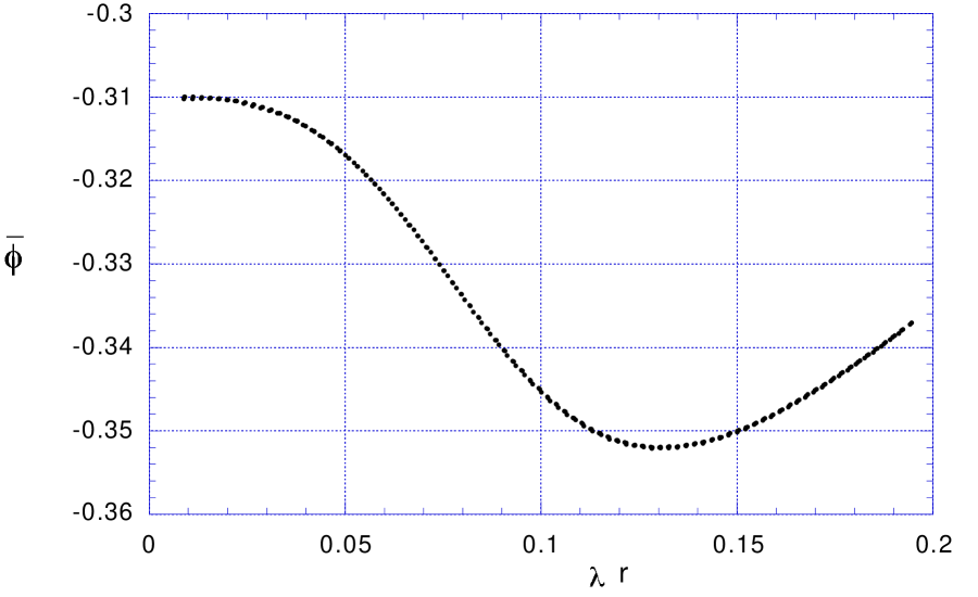
FIG. 2.: The scalar field is plotted as a function of rescaled radius

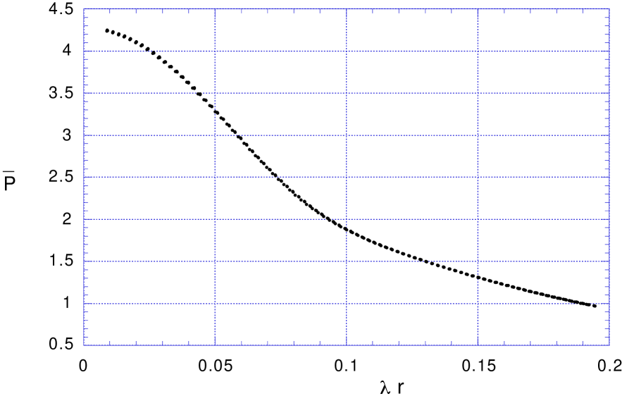
FIG. 3.: The rescaled time derivative of the scalar field is plotted as a function of rescaled radius

We now consider whether maximal slicing is compatible with the Choptuik critical solution. The maximal slices are generated numerically as described in the previous section. Compatibility of the foliation means that on corresponding slices, $\bar{\phi}$ and $\bar{P}$ as functions of $\lambda r$ are the same. Note that this is all that one needs to check, since in spherical symmetry the metric variables are determined by the matter variables. In figure 2, $\bar{\phi}$ is plotted vs. $\lambda r$ for three corresponding slices (those with $\phi_{0}$ halfway between zero and its minimum). These slices correspond to $\lambda=22.475,\,706.33$ and $22361$. Note that the three different curves are essentially indistinguishable, so $\bar{\phi}$ is the same on corresponding slices. In figure 3, $\bar{P}$ is plotted for these slices. Once again, the three curves are essentially indistinguishable, so $\bar{P}$ is the same on all three slices. It then follows that maximal slicing is compatible with the Choptuik critical solution.

This numerical study looks only at the case of the massless, minimally coupled, spherically symmetric scalar field. Nonetheless, we now argue that maximal slicing is always compatible in the case of spherical symmetry, and may be compatible in the case of axisymmetry or no symmetry. Let $g_{ab}$ be a periodically self-similar metric with associated diffeomorphism $\zeta$. Let $\Sigma$ be a maximal slice. Since ${\zeta^{*}}({g_{ab}})={e^{-2\Delta}}\,{g_{ab}}$, it follows that $\zeta(\Sigma)$ is a maximal slice. Therefore there must be a compatible maximal slicing that includes $\Sigma$. If the metric is spherically symmetric, there is a unique spherically symmetric maximal slicing. Therefore, this maximal slicing must be compatible. In the case of axisymmetry or no symmetry, things are more complicated because maximal slicing is no longer unique. The condition on the lapse $N$ that preserves maximal slicing is

$${D_{a}}{D^{a}}N\;+\;N\,\left[{R_{ab}}{n^{a}}{n^{b}}\,+\,R\,-\,{{}^{(3)}R}\right]=0\;\;\;.$$

Solutions of this equation are determined by boundary conditions. For gravitational collapse, the usual condition is that $N\to 1$ at infinity. Perhaps this condition leads to a compatible maximal slicing. The work of reference[6] on scaling in axisymmetric vacuum collapse uses maximal slicing with this condition on the lapse and finds that this foliation is compatible. It therefore seems likely that maximal slicing with $N\to 1$ at infinity in general leads to a compatible slicing. In any case, there is some maximal slicing that is compatible, even in the absence of symmetry. In this foliation, with our scale invariant variables, critical gravitational collapse is simply a limit cycle of a dynamical system.

IV Acknowledgements

We would like to thank Alan Rendall, Carsten Gundlach and Chuck Evans for helpful discussions. This work was partially supported by NSF grant PHY-9722039 and by a Cottrell College Science Award of Research Corporation to Oakland University. Part of this work was performed by KM in partial fulfillment of the requirements for the MS in Physics degree at Oakland University.

REFERENCES

- [1] D. Garfinkle, Phys. Rev. D56, R3169 (1997)
- [2] M. Choptuik, Phys. Rev. Lett. 70, 9 (1993)
- [3] C.R. Evans and J.S. Coleman, Phys. Rev. Lett. 72, 1782 (1994)
- [4] E.W. Hirschmann and D.M. Eardley, Phys. Rev. D51, 4198 (1995)
- [5] D. Garfinkle, Phys. Rev. D51, 5558 (1995)
- [6] A.M. Abrahams and C.R. Evans, Phys. Rev. Lett. 70, 2980 (1993)
- [7] R.S. Hamade, J.H. Horne and J.M. Stewart, Class. Quantum Grav. 13, 2241 (1996)
- [8] M. Choptuik, T. Chmaj and P. Bizon, Phys. Rev. Lett. 77, 424 (1996)
- [9] J. Traschen, Phys. Rev. D50, 7144 (1994)
- [10] S. Hod and T. Piran, Phys. Rev. D55, 3485 (1997)
- [11] D. Garfinkle and G. C. Duncan, gr-qc/9802061
- [12] C. Gundlach, gr-qc/9710066
- [13] T. Koike, T. Hara and S. Adachi, Phys. Rev. Lett. 74, 5170 (1995), T. Hara, T. Koike and S. Adachi, gr-qc/9607010
- [14] C. Gundlach, Phys. Rev. D55, 695 (1997)
- [15] S. Hod and T. Piran, Phys. Rev. D55, 440 (1997)
- [16] D. Christodoulou, Commun. Math. Phys. 105, 337 (1986)
- [17] C. Gundlach and J. Martin-Garcia, Phys. Rev. D54, 7353 (1996)
- [18] C. Gundlach, Phys. Rev. D55, 6002 (1997)
- [19] D.S. Goldwirth and T. Piran, Phys. Rev. D36, 3575 (1987)