Stability under radiation reaction of circular equatorial orbits around Kerr black holes

Abstract

We examine the evolution, under gravitational radiation reaction, of slightly eccentric equatorial orbits of point particles around Kerr black holes. Our method involves numerical integration of the Sasaki-Nakamura equation. It is discovered that such orbits decrease in eccentricity throughout most of the inspiral, until shortly before the innermost stable circular orbit (ISCO), when a critical radius $r_{\text{crit}}$ is reached beyond which the inspiralling orbits increase in eccentricity. It is shown that the number of orbits remaining in this last (eccentricity increasing) phase of the inspiral is an order of magnitude less for prograde orbits around rapidly spinning black holes than for retrograde orbits. In the extreme limit of a Kerr black hole with spin parameter $a=1$, this critical radius descends into the “throat” of the black hole.

I Introduction

Gravitational waves emitted by solar-mass-size compact bodies orbiting massive ($10^{6}M_{\odot}$ and greater) black holes (and spiralling towards them as they lose energy and angular momentum to the emitted radiation) are a favoured source for gravitational wave detectors sensitive to low-frequency radiation, such as proposed space-based detectors like the Laser Interferometer Space Antenna (LISA) [1]. Systems of this type lend themselves to theoretical analysis via perturbation theory, because of the extreme mass ratio between the two bodies. In recent years, the Teukolsky perturbation formalism for black holes has been employed successfully to describe orbital decay of small bodies orbiting a large Schwarzschild (i.e. non-rotating) black hole [2, 3, 4], using a mixture of analytic and numerical results (for an informative overview of much of the purely analytic work to date, see Mino et al. [5]). One result of this work has been to modify the long-standing result [6] that, under radiation reaction, orbits tend to become more circular as they slowly decay. In fact, inside a critical radius, which is $r_{\text{crit}}=6.6792M$ for nearly circular orbits in the Schwarzschild geometry, non-circular orbits tend to become more, rather than less, eccentric [2]. Although a precisely circular orbit would remain circular inside the critical radius, its circularity is no longer stable to small perturbations away from precise circularity as the orbital decay continues.

Despite their intrinsic interest, these results may prove of limited usefulness for any future low-frequency gravitational wave detectors, since there is no reason to expect that large black holes should typically have no spin at all. Just the opposite (that they should exhibit strong rotation) is perhaps more to be expected [7]. Therefore it is of great interest to extend this type of analysis to the case of rotating, or Kerr black holes. This presents no difficulty for the Teukolsky perturbation formalism itself, which was developed for the Kerr metric, but a problem does arise in dealing with an additional constant of the motion which governs orbits around spinning black holes. Unlike the energy and angular momentum, whose flux can easily be determined from the waves far from the source, until very recently there was no clear understanding of how to calculate the amount of “Carter constant” carried away by the emitted radiation. In spite of this, it has been shown recently, for general orbits in Kerr, that circular orbits (defined as orbits of constant Boyer-Lindquist radius, and sometimes referred to as “quasi-circular”) remain circular under radiation reaction [8, 9, 10]. While progress continues in developing techniques for dealing with general orbits in Kerr [11, 12, 13], it now seems worthwhile to investigate the case of nearly-circular, equatorial orbits around rotating black holes [14]. Equatorial orbits in the Kerr spacetime, like orbits in Schwarzschild, can be said to have zero “Carter constant”, which remains unchanged during orbital decay. Looking at these orbits can tell us if the behaviour previously observed for slightly-eccentric orbits in Schwarzschild is also seen in the Kerr metric for all values of the Kerr spin parameter $0\leq a\leq 1$.

It is shown in this paper that, for equatorial orbits, it is generally true that a critical radius, $r_{\text{crit}}$ exists beyond which slightly eccentric orbits become less circular due to radiation reaction, and that this radius is encountered close to the radius of the innermost stable circular orbit (ISCO). This is best illustrated by examining the behavior of the parameter $c=r_{0}\dot{e}/e\dot{r_{0}}$, where $e$ is the orbital eccentricity, and $r_{0}$ the mean radius, and an overdot indicates differentiation by time. This parameter is negative for orbits evolving with increasing eccentricities, and positive for decreasing eccentricity. Near the ISCO one can show, as in Sec. 9 below, that $c$ diverges towards negative infinity near the ISCO, for nearly all values of $a$. There is an apparent exception to this behaviour in the limiting case of a maximally rotating Kerr black hole with $a=M$. In that case, the horizon and the ISCO are both located at $r=M$ in Boyer-Lindquist co-ordinates, although they are still separate in terms of proper radial distance. As one approaches $r=M$, for the case of a prograde orbit around an extreme Kerr black hole, $c$ is both postive and finite, approaching the limit of $3/2$ at $r=M$. Not surprisingly therefore, for prograde orbits around black holes with very large $a>.99M$, the transition to eccentricity-increasing inspiral takes place only shortly before the onset of dynamical instability at the ISCO in terms of the Boyer-Lindquist radial co-ordinate. The number of orbits remaining at this point is an order of magnitude fewer for such cases than it is for retrograde orbits in the same geometry.

Since the radius of the ISCO is much smaller for prograde than for retrograde orbits (with $a=M$, $r_{\text{ISCO}}=M$ for prograde orbits and $r_{\text{ISCO}}=9M$ for retrograde orbits), the critical radius is also much smaller for prograde orbits. These results demonstrate that the onset of “back reaction instability” for circular orbits precedes, and is intimately connected with, the onset of dynamical instability signified by the ISCO. It seems reasonable to conjecture that the alteration in the shape of the radial protential as the ISCO approaches, at which point the minimum of the effective potential vanishes, is reponsible for the gain in eccentricity.

The organisation of the paper is as follows. In section 2, the orbital equations for geodesic motion (i.e. not including radiation reaction) are solved analytically for slightly eccentric, equatorial orbits. In section 3 the Tuekolsky perturbation formalism is described, and section 4 shows how to calculate the fluxes of energy and angular momentum carried away from the system using this formalism. In section 5 the Sasaki-Nakamura equation, which is actually solved rather than the Tuekolsky radial equation for numerical reasons, is presented. In section 6 the Teukolsky source function is calculated for a perturbing particle following the orbits of section 2, and the results of both of these sections come together in section 7 to yield the rate of change of orbital eccentricity due to radiation damping. This orbital evolution is described under the assumption of adiabaticity (that the orbital evolution is much slower than the orbital period), which introduces constraints which are discussed in section 8. Finally, in section 9, the analytic and numerical results are presented, followed by a discussion of their significance in section 10. A guide to the essential points of the argument is given at the end of section 7.

II Description of the orbit

Since the perturbation of the Kerr metric producing the gravitational waves is that of a small particle orbiting the black hole, it will be necessary to solve the orbital equations for a particle in orbit around a rotating black hole. We require expressions for $r(t)$, $\phi(t)$ and $\theta(t)$ to describe the orbit in Boyer-Lindquist co-ordinates. Since we restrict ourselves to equatorial orbits, the solution for the $\theta$ motion is trivial, $\theta=\pi/2$ is a constant throughout. The equatorial orbital equations for a particle in the Kerr spacetime, in these co-ordinates (leaving aside the trivial $d\theta/d\tau=0$), are well known [15]

$$\mu\Sigma^{2}dr/d\tau = [(E(r^{2}+a^{2})-aL_{z})^{2}-\Delta(\mu^{2}r^{2}+(L_{z}-aE)^{2})]^{1\over 2}\equiv\sqrt{R}$$ (1)

$$\mu\Sigma^{2}d\phi/d\tau = -(aE-L_{z}/\sin^{2}\theta)+(a/\Delta)(E(r^{2}+a^{2})-aL_{z})\equiv\Phi$$ (2)

$$\mu\Sigma^{2}dt/d\tau = -a(aE\sin^{2}\theta-L_{z})+{(r^{2}+a^{2})\over\Delta}(E(r^{2}+a^{2})-aL_{z})\equiv T,$$ (3)

where $\tau$ is proper time, $\Sigma=r^{2}+a^{2}\cos^{2}\theta$, $\Delta=r^{2}-2Mr+a^{2}$, and the black hole’s spin parameter $a$ is defined for convenience as $a=\vec{J}\cdot\hat{L}/M$, with $\vec{J}$ the spin angular momentum vector of the black hole, and $\hat{L}$ a unit vector pointing in the direction of the particle’s orbital angular momentum vector. For prograde orbits (in which the particle orbits in the same sense as the black hole’s spin) $a$ is positive, and for retrograde orbits (in which the particle rotates in the opposite sense to the hole), $a$ is negative. Recall that we restrict attention to equatorial orbits only, so that $\vec{J}$ and $\hat{L}$ are either parallel or anti-parallel. It is a condition of the perturbation scheme that $\mu/M\ll 1$, where $M$ is the mass of the central black hole and $\mu$ the mass of the orbiting particle. Finally, $E$ and $L_{z}$ are the particle’s orbital energy and angular momentum, respectively.

We now consider slightly eccentric orbits, and define a mean radius $r_{0}$, so that $\partial(R/r_{0}^{4})/\partial r|_{r=r_{0}}=0$. The eccentricity $e$ is defined so that $R(r=r_{0}(1+e))=0$. These definitions are chosen so that as $e\rightarrow 0$, $r_{0}$ reduces to the constant radius of a circular orbit, and so that $e$ corresponds, when $e\ll 1$ and in the appropriate limits, to definitions of the eccentricity of an orbit commonly used in the Schwarzschild geometry and in Newtonian mechanics [2]. These defining equations for $r_{0}$ and $e$ permit us to write the orbital energy and angular momentum in terms of these two quantities. Since we assume throughout that $e$ is a small quantity, it is convenient to expand $E$ and $L_{z}$ in terms of it,

$$E(r_{0},e) = E_{0}(r_{0})+eE_{1}(r_{0})+e^{2}E_{2}(r_{0})+e^{3}E_{3}(r_{0})+O(e^{4})$$ (4)

$$L_{z}(r_{0},e) = L_{0}(r_{0})+eL_{1}(r_{0})+r^{2}L_{2}(r_{0})+e^{3}L_{3}(r_{0})+O(e^{4}).$$ (5)

Using our two equations in $r_{0}$ and $e$, it is easy to show that

$$E_{0} = \mu{1-2v^{2}+qv^{3}\over(1-3v^{2}+2qv^{3})^{1\over 2}}$$ (6)

$$E_{1} = 0$$ (7)

$$E_{2} = \mu{v^{2}(1-3v^{2}+qv^{3}+q^{2}v^{4})(1-6v^{2}+8qv^{3}-3q^{2}v^{4})\over 2(1-3v^{2}+2qv^{3})^{3\over 2}(1-2v^{2}+q^{2}v^{4})}$$ (8)

$$E_{3} = -\mu{v^{2}(1-3v^{2}+qv^{3}+q^{2}v^{4})(1-7v^{2}+10qv^{3}-4q^{2}v^{4})\over(1-3v^{2}+2qv^{3})^{3\over 2}(1-2v^{2}+q^{2}v^{4})}$$ (9)

$$L_{0} = \mu{r_{0}v(1-2qv^{3}+q^{2}v^{4})\over(1-3v^{2}+2qv^{3})^{1\over 2}}$$ (10)

$$L_{1} = 0$$ (11)

$$L_{2} = \mu{qr_{0}v^{5}(q-3v+qv^{2}+q^{2}v^{3})(1-6v^{2}+8qv^{3}-3q^{2}v^{4})\over 2(1-3v^{2}+2qv^{3})^{3\over 2}(1-2v^{2}+q^{2}v^{4})}$$ (12)

$$L_{3} = -\mu{qr_{0}v^{5}(q-3v+qv^{2}+q^{2}v^{3})(1-7v^{2}+10qv^{3}-4q^{2}v^{4})\over(1-3v^{2}+2qv^{3})^{3\over 2}(1-2v^{2}+q^{2}v^{4})}.$$ (13)

Here $v=\sqrt{M/r_{0}}$ and $q=a/M$. These results, up to order $e^{2}$ are given in Ref. [14].

We wish to write the change in the eccentricity brought about by the loss of orbital angular momentum and energy, in terms of the rates of loss of those two quantities. Since we have $E$ and $L_{z}$ as functions of $r_{0}$ and $e$, we use the chain rule for differentiation to write

$$\dot{E} = -dE_{GW}/dt={\partial E\over\partial e}\dot{e}+{\partial E\over\partial r_{0}}\dot{r}_{0}$$ (14)

$$\dot{L}_{z} = -dL_{GW}/dt={\partial L_{z}\over\partial e}\dot{e}+{\partial L_{z}\over\partial r_{0}}\dot{r}_{0},$$ (15)

where $dE_{GW}/dt$ and $dL_{GW}/dt$ are the total energy and angular momentum carried towards infinity and the black hole horizon per unit time by the gravitational waves, averaged over several wavelengths. We will write these quantities also in terms of $e$ and $r_{0}$,

$${dE_{GW}\over dt} = \dot{E}_{0}+e\dot{E}_{1}+e^{2}\dot{E}_{2}+O(e^{3})$$ (16)

$${dL_{GW}\over dt} = \dot{L}_{0}+e\dot{L}_{1}+e^{2}\dot{L}_{2}+O(e^{3}).$$ (17)

As we shall find later, $\dot{E}_{1}=\dot{L}_{1}=0$. Eliminating $r_{0}$ from Eq. (15), we derive

$$\dot{e}=[-{dE_{GW}\over dt}L_{z}^{\prime}+{dL_{GW}\over dt}E^{\prime}]/[{\partial E\over\partial e}L_{z}^{\prime}-{\partial L_{z}\over\partial e}E^{\prime}],$$ (18)

where $\prime\equiv\partial/\partial r_{0}$.

Substiting Eqs. (17) and (5) into Eq. (18), we find, keeping terms up to order $e^{2}$,

$$\dot{e}={-L_{0}^{\prime}(\dot{E}_{0}-{E_{0}^{\prime}\over L_{0}^{\prime}}\dot{L}_{0})-e^{2}L_{0}^{\prime}(\dot{E}_{2}-{E_{0}^{\prime}\over L_{0}^{\prime}}\dot{L}_{2})-e^{2}L_{2}^{\prime}(\dot{E}_{0}-{E_{2}^{\prime}\over L_{2}^{\prime}}\dot{L}_{0})\over 2e(E_{2}L_{0}^{\prime}-L_{2}E_{0}^{\prime})}.$$ (19)

Now, from Eqs. (13), we see that

$${E_{0}^{\prime}\over L_{0}^{\prime}}={\sqrt{M}\over r_{0}^{3\over 2}+a\sqrt{M}}=\Omega,$$ (20)

where $\Omega$ is the angular frequency of a circular orbit of radius $r_{0}$. It follows from an interesting (and quite general [16]) characteristic of circular orbits, and will be shown later in this case that, the circular (i.e. zeroth order in the eccentricity) rates of loss of energy and angular momentum are related by

$$\dot{E}_{0}=\Omega\dot{L}_{0}.$$ (21)

Therefore

$$\mu\dot{e}=-ej(v)[g(v)\dot{E}_{0}+\dot{E}_{2}-\Omega\dot{L}_{2}],$$ (22)

where

$$j(v)={\mu\over E_{2}-\Omega L_{2}}={(1+qv^{3})(1-2v^{2}+q^{2}v^{4})(1-3v^{2}+2qv^{3})^{1\over 2}\over v^{2}(1-6v^{2}+8qv^{3}-3q^{2}v^{4})}$$ (23)

and

$$g(v)={L_{2}^{\prime}\over L_{0}^{\prime}}-{E_{2}^{\prime}\over E_{0}^{\prime}}={{\cal G}(v)\over 2(1+qv^{3})(1-6v^{2}+8qv^{3}-3q^{2}v^{4})(1-2v^{2}+q^{2}v^{4})^{2}},$$ (24)

where

$${\cal G}(v)=2 - 27v^{2}+72v^{4}-36v^{6}+38qv^{3}-17q^{2}v^{4}-144qv^{5}+86q^{2}v^{6}$$ (25)

$$+ 4q^{3}v^{7}+72qv^{7}-12q^{4}v^{8}-36q^{2}v^{8}-23q^{4}v^{10}+30q^{5}v^{11}$$ (26)

$$- 9q^{6}v^{12}$$ (27)

Since $\dot{e}$ is proportional to $e$ in this equation, it is plain that a precisely circular orbit (one with $e=0$), will remain circular under radiation reaction, provided that we can indeed show that $\dot{E}_{0}=\Omega\dot{L}_{0}$ and $\dot{E}_{1}=\dot{L}_{1}=0$. It is also plain that the question of the stability of an orbit’s circularity will be determined by the sign of Eq. (22), which requires us to calculate the loss of orbital energy and angular momentum up to second order in $e$.

Similarly we can solve for $\dot{r}_{0}$, the rate of change of the orbital radius, which tells us that to leading order $\dot{r}_{0}=-\dot{E}_{0}/E^{\prime}_{0}$, which implies that

$$\mu\dot{r}_{0}/r_{0}=-{2(1-3v^{2}+2qv^{3})^{3/2}\over v^{2}(1-6v^{2}+8qv^{3}-3q^{2}v^{4})}\dot{E}_{0}.$$ (28)

With this in hand it is possible to proceed to the solution of the geodesic equations [Eqs. (3)]. We expand $r(t)$ about the mean radius $r_{0}$ in terms of the small eccentricity $e$, so that

$$r(t)=r_{0}[1+er_{1}(t)+e^{2}r_{2}(t)+O(e^{3})].$$ (29)

Making use of the expansions of $E$, $L_{z}$ and $r(t)$ in terms of $e$, we expand out the equation $(dr/dt)^{2}=R/T^{2}$, and collect terms of order $e^{2}$ and $e^{3}$ (note that the $e^{3}$ term in $r(t)$ does not contribute until $O(e^{4})$ in $R/T^{2}$), giving us two differential equations,

$$(dr_{1}/dt)^{2}=\Omega_{r}^{2}(1-r_{1}^{2}),$$ (30)

where we define a radial frequency,

$$\Omega_{r}=\Omega(1-6v^{2}+8qv^{3}-3q^{2}v^{4})^{1\over 2}$$ (31)

and

$${1\over\Omega_{r}^{2}}{dr_{1}\over dt}{dr_{2}\over dt}+r_{1}r_{2}=f_{1}(v)+f_{2}(v)r_{1}+f_{3}(v)r_{1}^{3},$$ (32)

where

$$f_{1}(v) = -{1-7v^{2}+10qv^{3}-4q^{2}v^{4}\over 1-6v^{2}+8qv^{3}-3q^{2}v^{4}}$$ (33)

$$f_{2}(v) = {2v^{2}(1-2qv^{3}+q^{2}v^{4})\over(1+qv^{3})(1-2v^{2}+q^{2}v^{4})}$$ (34)

$$f_{3}(v) = {{\cal F}_{3}(v)\over(1+qv^{3})(1-2v^{2}+q^{2}v^{4})(1-6v^{2}+8qv^{3}-3q^{2}v^{4})},$$ (35)

and

$${\cal F}_{3}(v)=1 - 11v^{2}+26v^{4}+11qv^{3}-3q^{2}v^{4}-41qv^{5}+15q^{2}v^{6}$$ (36)

$$- 10qv^{7}+7q^{3}v^{7}+24q^{2}v^{8}-4q^{4}v^{8}-27q^{3}v^{9}+16q^{4}v^{10}$$ (37)

$$- 4q^{5}v^{11}.$$ (38)

Integrating these equations in order, we find,

$$r_{1}(t) = \cos(\Omega_{r}t)$$ (39)

$$r_{2}(t) = -f_{1}(v)(1-\cos(\Omega_{r}t))+{1\over 2}f_{3}(v)(1-\cos(2\Omega_{r}t)).$$ (40)

It remains to solve for the $\phi$-motion. Again we expand out the geodesic equation $d\phi/dt=\Phi/T$, integration of which yields

$$\phi(t)=\Omega_{\phi}t-ep(v)\sin(\Omega_{r}t)+O(e^{2}),$$ (41)

where

$$p(v)={2(1-3v^{2}+2qv^{3})\over[(1+qv^{3})(1-2v^{2}+q^{2}v^{4})(1-6v^{2}+8qv^{3}-3q^{2}v^{4})^{1/2}]}$$ (42)

and

$$\Omega_{\phi} = \Omega\Bigl{[}1$$ (43)

$$- {3(1-11v^{2}+24v^{4}+13qv^{3}-4q^{2}v^{4}-46qv^{5}+25q^{2}v^{6}+q^{3}v^{7}-3q^{4}v^{8})\over 2(1+qv^{3})(1-2v^{2}+q^{2}v^{4})(1-6v^{2}+8qv^{3}-3q^{2}v^{4})}e^{2}$$ (44)

$$+ O(e^{3})\Bigr{]}$$ (45)

$$\equiv \Omega[1-\Delta\Omega e^{2}+O(e^{3})]$$ (46)

is the azimuthal angular frequency. The $O(e^{2})$ part of $\phi(t)$ which is proportional to $\sin(\Omega_{r}t)$ is not given, as neither it nor the $O(e^{2})$ part of $r(t)$ contribute to the final result for $\dot{e}$, for reasons which will become clear later. Only the $O(e^{2})$ part of $\Omega_{\phi}$ (i.e. $\Delta\Omega$) is required, although it is necessary to know $r_{2}(t)$ to derive $\Delta\Omega$.

III The Teukolsky formalism

We employ a scheme previously used in the Schwarzschild case to investigate the evolution of slightly eccentric orbits under radiation reaction [2]. This scheme is based on the Teukolsky formalism for perturbations of the Kerr metric. In this formalism one can decompose the Weyl scalar $\psi_{4}$ (which describes gravitational wave fluxes near infinity for such a system) as follows,

$$\psi_{4}={1\over(r-ia\cos\theta)^{4}}\int^{+\infty}_{-\infty}\sum_{lm}R_{lm\omega}(r)\mbox{}_{-2}S_{lm}^{a\omega}(\theta)e^{im\phi}e^{-i\omega t}d\omega,$$ (47)

where $\mbox{}_{-2}S_{lm}^{a\omega}$ is the spheroidal harmonic function of spin weight $s=-2$. The normalization used here for these functions is $\int^{\pi}_{0}|\mbox{}_{-2}S_{lm}^{a\omega}(\theta)|^{2}\sin\theta d\theta=1/2\pi$. The radial function $R_{lm\omega}(r)$ obeys the Teukolsky equation,

$$\Delta^{2}{d\over dr}\Bigl{(}{1\over\Delta}{dR_{lm\omega}\over dr}\Bigr{)}-V(r)R_{lm\omega}(r)=T_{lm\omega}(r),$$ (48)

where $T_{lm\omega}$ is the Teukolsky source function, to be evaluated below. The Teukolsky potential is defined by

$$V(r)=-{K^{2}+4i(r-M)K\over\Delta}+8i\omega r+\lambda,$$ (49)

where $K=(r^{2}+a^{2})\omega-ma$ and $\lambda$ is the eigenvalue associated with the appropriate spheroidal harmonic $\mbox{}_{-2}S^{a\omega}_{lm}$.

We can define two solutions to the homogeneous Teukolsky equation, $R^{H}_{lm\omega}(r)$ and $R^{\infty}_{lm\omega}(r)$, with the following boundary conditions,

$$R^{H}_{lm\omega} \sim \Delta^{2}e^{ikr^{*}},\text{as}\quad r\rightarrow r_{+}$$ (50)

$$R^{H}_{lm\omega} \sim r^{3}B^{\text{out}}_{lm\omega}e^{i\omega r^{*}}+{1\over r}B^{\text{in}}_{lm\omega}e^{-i\omega r^{*}},\text{as}\quad r\rightarrow\infty$$ (51)

and

$$R^{\infty}_{lm\omega} \sim D^{\text{out}}e^{ikr^{*}}+\Delta^{2}D^{\text{in}}e^{-ikr^{*}},\text{as}\quad r\rightarrow r_{+}$$ (52)

$$R^{\infty}_{lm\omega} \sim r^{3}e^{-i\omega r^{*}},\text{as}\quad r\rightarrow\infty,$$ (53)

where $k=\omega-ma/(2Mr_{+})$, $r_{+}=M+\sqrt{M^{2}-a^{2}}$ is the radius of the black hole horizon, and $r^{*}$, the tortoise co-ordinate, is defined as

$$r^{*}=r+{2Mr_{+}\over r_{+}-r_{-}}\ln{r-r_{+}\over 2M}-{2Mr_{-}\over r_{+}-r_{-}}\ln{r-r_{-}\over 2M},$$ (54)

where $r_{-}=M-\sqrt{M^{2}-a^{2}}$.

From Ref. [17], the solution of the Teukolsky equation (solved via a retarded Green’s function) is

$$R_{lm\omega}(r)=R^{\infty}_{lm\omega}(r)Z^{H}(r)+R^{H}_{lm\omega}(r)Z^{\infty}(r),$$ (55)

where

$$Z^{H}(r)={1\over 2i\omega B^{\text{in}}_{lm\omega}}\int^{r}_{r_{+}}{R^{H}_{lm\omega}(r)T_{lm\omega}(r)\over\Delta^{2}}dr$$ (56)

and

$$Z^{\infty}(r)={1\over 2i\omega B^{\text{in}}_{lm\omega}}\int^{\infty}_{r}{R^{\infty}_{lm\omega}(r)T_{lm\omega}(r)\over\Delta^{2}}dr.$$ (57)

For convenience, we will write $Z^{H}_{lm\omega}=Z^{H}(r\rightarrow\infty)$ and $Z^{\infty}_{lm\omega}=Z^{\infty}(r\rightarrow r_{+})$, and therefore our two solutions can be written as

$$R_{lm\omega}(r\rightarrow\infty)\sim Z^{H}_{lm\omega}r^{3}e^{i\omega r^{*}}$$ (58)

and

$$R_{lm\omega}(r\rightarrow r_{+})\sim Z^{\infty}_{lm\omega}\Delta^{2}e^{-ikr^{*}}.$$ (59)

IV Energy and angular momentum fluxes

Towards infinity, the Weyl scalar can be related to the two fundamental polarizations of gravitational waves by

$$\psi_{4}={1\over 2}(\ddot{h}_{+}-i\ddot{h}_{\times}).$$ (60)

From this and Eq. (47) above, we can determine the averaged energy and angular momentum fluxes at infinity, employing the Isaacson stress-energy tensor to define the energy flux in the wave [18], as

$$\langle{dE_{\text{GW}}\over dt}\rangle=\dot{E}^{\infty}=\sum_{lmk}{|Z^{H}_{lmk}|^{2}\over 4\pi\omega_{k}^{2}}$$ (61)

and

$$\langle{dL_{\text{GW}}\over dt}\rangle=\dot{L}_{z}^{\infty}=\sum_{lmk}{m|Z^{H}_{lmk}|^{2}\over 4\pi\omega_{k}^{3}},$$ (62)

where the amplitude coefficient is decomposed into a discrete set of frequencies based on the particle’s orbital motion,

$$Z^{H}_{lm\omega}=\sum_{k}Z^{H}_{lmk}\delta(\omega-\omega_{k}).$$ (63)

Energy and angular momentum are also lost by radiation through the horizon of the central black hole. Again, $\psi_{4}$ completely describes the waves as $r^{*}\rightarrow-\infty$ and, with Teukolsky and Press [19], we find

$$\dot{E}^{H}=\sum_{lmk}\alpha^{k}_{l}{|Z^{\infty}_{lmk}|^{2}\over 4\pi\omega^{2}_{k}}$$ (64)

and

$$\dot{L}^{H}_{z}=\sum_{lmk}\alpha^{k}_{l}{m|Z^{\infty}_{lmk}|^{2}\over 4\pi\omega^{3}_{k}},$$ (65)

with an identical decompostion of $Z^{\infty}_{lm\omega}$ as with $Z^{H}_{lm\omega}$, and where

$$\alpha^{k}_{l}={2^{8}w_{k}^{7}k(k^{2}+4\epsilon^{2})(k^{2}+16\epsilon^{2})(2Mr_{+})^{5}\over|C|^{2}}$$ (66)

and $\epsilon=\sqrt{M^{2}-a^{2}}/4Mr_{+}$ and

$$|C|^{2} = [(\lambda+2)^{2}+4a\omega m-4a^{2}\omega^{2}](\lambda^{2}+36a\omega m-36a^{2}\omega^{2})$$ (67)

$$+ (2\lambda+3)(96a^{2}\omega^{2}-48a\omega m)+144\omega^{2}(M^{2}-a^{2}).$$ (68)

The total rates of loss of energy and angular momentum by the system are $\dot{E}^{H}+\dot{E}^{\infty}$ and $\dot{L}^{H}_{z}+\dot{L}^{\infty}_{z}$.

V The Sasaki-Nakamura equation

The preceding section makes it clear that our chief task is to calculate the amplitudes $Z^{H,\infty}_{lmk}$, and it is apparent from Eqs. (56) and (57) that this will entail solving the Teukolsky equation to find the amplitude of the in-going waves at infinity, $B^{\text{in}}_{lm\omega}$ from Eq. (51). Numerically this presents a problem, however, since the ingoing waves for this solution are completely swamped by the outoing waves at large radii [compare amplitudes of $B^{\text{out}}_{lm\omega}r^{3}$ and $B^{\text{in}}_{lm\omega}/r$ as $r\rightarrow\infty$ in Eq. (51)]. In the Schwarzschild case this problem is typically avoided by solving instead the Regge-Wheeler equation, and transforming its solution to that of the Teukolsky equation via the Chandrasekhar transformation [20]. The virtue of this is that in the Regge-Wheeler formalism, with its short-range potential, the ingoing and outgoing waves near infinity have the same order of magnitude.

In the Kerr case Sasaki and Nakamura have found an equation with the same useful properties as the Regge-Wheeler equation in Schwarzschild which, moreover, reduces to the latter equation when $a\rightarrow 0$ [21]. The Sasaki-Nakamura equation is written as follows

$${d^{2}X_{lm\omega}\over dr^{2}}-F(r){dX_{lm\omega}\over dr}-U(r)X_{lm\omega}=0.$$ (69)

The functions $F(r)$ and $U(r)$ are given in the appendix. The equivalents to our two solutions to the Teukolsky equation are

$$X^{H}_{lm\omega} \sim A^{\text{out}}_{lm\omega}e^{i\omega r^{*}}+A^{\text{in}}_{lm\omega}e^{-i\omega r^{*}},\text{as}\quad r\rightarrow\infty$$ (70)

$$X^{H}_{lm\omega} \sim e^{-ikr^{*}},\text{as}\quad r\rightarrow r_{+}$$ (71)

and

$$X^{\infty}_{lm\omega} \sim e^{i\omega r^{*}},\text{as}\quad r\rightarrow\infty$$ (72)

$$X^{\infty}_{lm\omega} \sim D^{\text{out}}e^{ikr^{*}}+D^{\text{in}}e^{-ikr^{*}},\text{as}\quad r\rightarrow r_{+}.$$ (73)

The transformations between the quantities we require are

$$R^{H}_{lm\omega} = {1\over\eta}[(\alpha+{\beta_{,r}\over\Delta})\chi^{H}_{lm\omega}-{\beta\over\Delta}\chi^{H}_{lm\omega,r}],$$ (74)

$$R^{\infty}_{lm\omega} = -{c_{0}\over 4\omega^{2}\eta}[(\alpha+{\beta_{,r}\over\Delta})\chi^{\infty}_{lm\omega}-{\beta\over\Delta}\chi^{\infty}_{lm\omega,r}],$$ (75)

and

$$B^{\text{in}}_{lm\omega}=-{1\over 4\omega^{2}}A^{\text{in}}_{lm\omega},$$ (76)

where $\chi^{H,\infty}_{lm\omega}=X^{H,\infty}_{lm\omega}\Delta/\sqrt{r^{2}+a^{2}}$, and $c_{0}$, $\alpha$, $\beta$ and $\eta$ are given in the appendix.

VI The source term

The Teukolsky source term is given by [22]

$$T_{lm\omega}=4\int\rho^{-5}\bar{\rho}^{-1}(B_{2}^{\prime}+B_{2}^{\prime*})e^{-im\phi+i\omega t}\mbox{}_{-2}S^{a\omega}_{lm}d\Omega dt,$$ (77)

where

$$B_{2}^{\prime} = -{1\over 2}\rho^{8}\bar{\rho}L_{-1}[\rho^{-4}L_{0}(\rho^{-2}\bar{\rho}^{-1}T_{nn})]$$ (78)

$$- {1\over 2\sqrt{2}}\rho^{8}\bar{\rho}\Delta^{2}L_{-1}[\rho^{-4}\bar{\rho}^{2}J_{+}(\rho^{-2}\bar{\rho}^{-2}\Delta^{-1}T_{\bar{m}n})],$$ (79)

$$B_{2}^{\prime*} = -{1\over 4}\rho^{8}\bar{\rho}J_{+}[\rho^{-4}J_{+}(\rho^{-2}\bar{\rho}T_{\bar{m}\bar{m}}]$$ (80)

$$- {1\over 2\sqrt{2}}\rho^{8}\bar{\rho}\Delta^{2}J_{+}[\rho^{-4}\bar{\rho}^{2}\Delta^{-1}L_{-1}(\rho^{-2}\bar{\rho}^{-2}T_{\bar{m}n})],$$ (81)

and $\rho=(r-ia\cos\theta)^{-1}$, with $\bar{\rho}$ its complex conjugate. The operators $L_{s}$ and $J_{+}$ are defined as

$$L_{s}=\partial_{\theta}+{m\over\sin\theta}-a\omega\sin\theta+s\cot\theta$$ (82)

and

$$J_{+}=\partial_{r}+i{K\over\Delta}.$$ (83)

The tetrad components of the particle’s energy momentum tensor can be written

$$T_{nn} = {C_{nn}\over\sin\theta}\delta(r-r(t))\delta(\theta-\pi/2)\delta(\phi-\phi(t)),$$ (84)

$$T_{\bar{m}n} = {C_{\bar{m}n}\over\sin\theta}\delta(r-r(t))\delta(\theta-\pi/2)\delta(\phi-\phi(t)),$$ (85)

$$T_{\bar{m}\bar{m}} = {C_{\bar{m}\bar{m}}\over\sin\theta}\delta(r-r(t))\delta(\theta-\pi/2)\delta(\phi-\phi(t)),$$ (86)

where

$$C_{nn} = C^{(0)}_{nn}+C^{(1)}_{nn}{dr\over dt}+C^{(2)}_{nn}({dr\over dt})^{2}$$ (87)

$$= {\mu\over 4\Sigma^{3}\dot{t}}[E(r^{2}+a^{2})-aL_{z}]^{2}+{\mu\over 2\Sigma^{2}}[E(r^{2}+a^{2})-aL_{z}]{dr\over dt}$$ (88)

$$+ {\mu\dot{t}\over 4\Sigma}({dr\over dt})^{2}$$ (89)

$$C_{\bar{m}n} = C^{(0)}_{\bar{m}n}+C^{(1)}_{\bar{m}n}{dr\over dt}$$ (90)

$$= {\mu\rho\over 2\sqrt{2}\Sigma^{2}\dot{t}}[E(r^{2}+a^{2})-aL_{z}][i\sin\theta(aE-{L_{z}\over\sin^{2}\theta})]$$ (91)

$$- {\mu\rho\over 2\sqrt{2}\Sigma}[i\sin\theta(aE-{L_{z}\over\sin^{2}\theta}]{dr\over dt}$$ (92)

$$C_{\bar{m}\bar{m}} = {\mu\rho^{2}\over 2\Sigma\dot{t}}[i\sin\theta(aE-{L_{z}\over\sin^{2}\theta})]^{2}$$ (93)

and $\dot{t}=dt/d\tau$.

Integrating by parts, and making use of the adjoint operator $L_{s}^{\dagger}=\partial_{\theta}-m/\sin\theta+a\omega\sin\theta+s\cot\theta=\partial_{\theta}+f(\theta)$, which bears the following useful relation to the operator $L_{s}$ defined above:

$$\int^{\pi}_{0}h(\theta)L_{s}[g(\theta)]\sin\theta d\theta=-\int^{\pi}_{0}g(\theta)L^{\dagger}_{1-s}[h(\theta)]\sin\theta d\theta,$$ (94)

with $g(\theta)$ and $h(\theta)$ arbitrary functions [14], we find that

$$T_{lm\omega} = \int^{\infty}_{-\infty}\int^{2\pi}_{0}\Delta^{2}[\{(A_{nn0}+A_{\bar{m}n0}+A_{\bar{m}\bar{m}0})\delta(r-r(t)\}$$ (95)

$$+ \{(A_{\bar{m}n1}+A_{\bar{m}\bar{m}1})\delta(r-r(t))\}_{,r}$$ (96)

$$+ \{A_{\bar{m}\bar{m}2}\delta(r-r(t))\}_{,rr}]\delta(\phi-\phi(t))e^{i\omega t-im\phi}d\phi dt.$$ (97)

The $A$’s are all functions of $r$ only, and in each case $A=A^{(0)}+A^{(1)}(dr/dt)+A^{(2)}(dr/dt)^{2}$, where (writing $\mbox{}_{-2}S^{a\omega}_{lm}$ simply as $S$ hereafter for simplicity)

$$A^{(i)}_{nn0} = -{2\over\Delta^{2}}C^{(i)}_{nn}r^{3}(rS_{,\theta\theta}-2iaS_{,\theta}+2rf(\pi/2)S_{,\theta}$$ (98)

$$- 2iaf(\pi/2)S+rS(f(\pi/2)^{2}-2),$$ (99)

$$A^{(i)}_{\bar{m}n0} = {2\sqrt{2}\over\Delta}C^{(i)}_{\bar{m}n}r^{3}(S_{,\theta}+f(\pi/2)S)(i{K\over\Delta}+{2\over r}),$$ (100)

$$A^{(0)}_{\bar{m}\bar{m}0} = -r^{2}C_{\bar{m}\bar{m}}S(-i({K\over\Delta})_{,r}-({K\over\Delta})^{2}+{2i\over r}{K\over\Delta}),$$ (101)

$$A^{(i)}_{\bar{m}n1} = {2\sqrt{2}\over\Delta}r^{3}C^{(i)}_{\bar{m}n}(S_{,\theta}+f(\pi/2)S),$$ (102)

$$A^{(0)}_{\bar{m}\bar{m}1} = -2r^{2}C_{\bar{m}\bar{m}}S(i{K\over\Delta}+{1\over r}),$$ (103)

$$A^{(0)}_{\bar{m}\bar{m}2} = -r^{2}C_{\bar{m}\bar{m}}S,$$ (104)

$$A^{(2)}_{\bar{m}n0} = A^{(2)}_{\bar{m}n1}=A^{(1)}_{\bar{m}\bar{m}0}=A^{(2)}_{\bar{m}\bar{m}0}=A^{(1)}_{\bar{m}\bar{m}1}=A^{(2)}_{\bar{m}\bar{m}1}=A^{(1)}_{\bar{m}\bar{m}2}=A^{(2)}_{\bar{m}\bar{m}2}=0.$$ (105)

In every case the spheroidal harmonic function ($S$) and its derivatives are evaluated at $\theta=\pi/2$.

It is now easy to show, from Eqs. (56) and (57) and using integration by parts (keeping in mind that we are interested only in closed orbits, for which $r_{+}<r<\infty$ always holds strictly), that

$$Z^{H,\infty}_{lm\omega}={1\over 2i\omega B^{\text{in}}_{lm\omega}}\int_{r_{+}}^{\infty}\int^{\infty}_{-\infty}\int^{2\pi}_{0}I^{H,\infty}_{lm\omega}(r)\delta(r-r(t))\delta(\phi-\phi(t))d\phi dtdr,$$ (106)

for which $I^{H,\infty}_{lm\omega}(r)=I^{(0)}_{lm\omega}(r)+I^{(1)}_{lm\omega}(r)(dr/dt)+I^{(2)}_{lm\omega}(r)(dr/dt)^{2}$, where

$$I^{(i)}_{lm\omega}(r)=R^{H,\infty}_{lm\omega}(A^{(i)}_{nn0}+A^{(i)}_{\bar{m}n0}+A^{(i)}_{\bar{m}\bar{m}0})-{dR^{H,\infty}_{lm\omega}\over dr}(A^{(i)}_{\bar{m}n1}+A^{(i)}_{\bar{m}\bar{m}1})+{d^{2}R^{H,\infty}_{lm\omega}\over dr^{2}}A^{(i)}_{\bar{m}\bar{m}2}.$$ (107)

It is necessary to expand $Z^{H,\infty}_{lm\omega}$ in terms of the eccentricity $e$, keeping in mind that we wish, as shown in section 2 above, to find $\dot{E}^{H,\infty}$ and $\dot{L}_{z}^{H,\infty}$ to second order in $e$, and that each of these is proportional to $|Z^{H,\infty}_{lm\omega}|^{2}$. However, it transpires that only terms up to order $e$ in the integrand of Eq. (106) contribute to order $e^{2}$ in $\dot{e}$, the rate of change of eccentricity derived from $\dot{E}^{H,\infty}$ and $\dot{L}_{z}^{H,\infty}$. The reasons for this emerge as we proceed to expand $I^{H,\infty}_{lm\omega}(r)$, $\delta(r-r(t))$ and $\delta(\phi-\phi(t))$ in powers of $e$.

Employing the expansions of $r(t)$ and $\phi(t)$ derived above [Eqs. (29) and (41)], we can write the product of delta functions in Eq. (106) as a product of two Taylor expansions in the small parameter $e$, about the points $r-r_{0}$ and $\phi-\Omega_{\phi}t$.

$$\delta(r-r(t))\delta(\phi-\phi(t)) = \delta(r-r_{0})\delta(\phi-\Omega_{\phi}t)-er_{0}\cos\Omega_{r}t\delta^{\prime}(r-r_{0})\delta(\phi-\Omega_{\phi}t)$$ (108)

$$- ep(r_{0})\sin\Omega_{r}t\delta^{\prime}(\phi-\Omega_{\phi}t)\delta(r-r_{0})+O(e^{2}),$$ (109)

where the prime denotes differentiation with respect to the function’s argument. We can integrate by parts in Eq. (106) to integrate terms containing derivatives of delta functions, and this will simply mean that $\delta^{\prime}(\phi-\Omega_{\phi}t)$ will be replaced by $im\delta(\phi-\Omega_{\phi}t)$, since $e^{-im\phi}$ is the only other part of the integrand which depends on $\phi$. Completing the $\phi$ integration thus leaves us with the overall factor $e^{i(\omega-m\Omega_{\phi})t}$, and some terms depending on $\cos\Omega_{r}t$, $\sin\Omega_{r}t$ and, in the $O(e^{2})$ part, on $\cos 2\Omega_{r}t$ and $\sin 2\Omega_{r}t$. Following the time integration, then, we will have a series of delta functions of the type $\delta(\omega-m\Omega_{\phi})$ [at all orders, except $O(e)$], $\delta(\omega-m\Omega_{\phi}\pm\Omega_{r})$ (at all orders from $O(e)$ up) and, in general, $\delta(\omega-m\Omega_{\phi}\pm k\Omega_{r})$ at $O(e^{k})$ and above.

These delta functions, after integration over $\omega$ to derive $\psi_{4}$ [Eq. (47)], produce terms representing energy and angular momentum emitted at the fundamental (circular motion) frequency $w_{m}=m\Omega_{\phi}$, and at a series of discrete sidebands, $w_{\pm}=m\Omega_{\phi}\pm\Omega_{r}$ and $w_{\pm k}=m\Omega_{\phi}\pm k\Omega_{r}$. The occurrence of these delta functions justifies the decomposition of $Z^{H,\infty}_{lm\omega}$ referred to earlier [Eq. (63) above].

It is, of course, $|Z^{H,\infty}_{lm\omega}|^{2}$ which is integrated in Eq. (47). Therefore, up to order $e^{2}$, only those $O(e^{2})$ terms in $Z^{H,\infty}_{lm\omega}$ which cross multiply with $O(e^{0})$ terms will contribute. Since the frequency must be single valued for any given term, only the circular harmonic ($w_{m}$) term in $O(e^{2})$ survives the Fourier transform which produces the Weyl scalar, all other terms being annihilated. The $O(e)$ terms in $Z$ have no circular harmonic term, as mentioned before, so these terms only contribute to loss of energy and engular momentum at $O(e^{2})$.

As seen from Eq. (22) above, it is the difference $\dot{E}_{2}-\Omega\dot{L}_{2}$ on which $\dot{e}$ actually depends at leading order. Eqs. (61),(62),(64) and (65) show that

$$\dot{E}_{n}-\Omega\dot{L}_{n}\propto 1-{m\Omega\over\omega_{k}},\quad\text{at order}\quad e^{n}$$ (110)

which is zero to leading order if $\omega_{k}=\omega_{m}=m\Omega_{\phi}$. This means not only that the $O(e^{2})$ terms in $Z^{H,\infty}_{lm\omega}$ do not contribute at all to $\dot{e}$ below $O(e^{3})$, but also that $\dot{E}_{0}-\Omega\dot{L}_{0}$ is also zero to leading order, as noted above [Eq. (21)]. In fact, since the eccentric correction to the azimuthal frequency $\Omega_{\phi}$ is itself of $O(e^{2})$, the circular losses of energy and angular momentum contribute to $\dot{e}$ at $O(e^{2})$ to leading order, like the first order terms in $Z$. Therefore there is no loss of $E$ and $L_{z}$ at $O(e)$, and so $\dot{E}_{1}=0$ and $\dot{L}_{1}=0$ as claimed in section 2.

This proves that a precisely circular equatorial orbit in Kerr will always remain circular under radiation reaction (as long as the adiabatic approximation still holds). Furthermore it means that to find the leading order correction to this condition for slightly eccentric orbits, and thus establish the stability of circularity, we need only examine the $O(e)$ terms in Eq. (47), and can drop all $O(e^{2})$ corrections to the motion, except for the $\Delta\Omega$ part of $\Omega_{\phi}$. This also means, of course, that only contributions to the loss of energy and angular momentum from the first pair of sidebands ($\omega=\omega_{\pm}$) need be included with the circular harmonic ($\omega_{m}$) in calculating $\dot{e}$ to leading order.

VII Calculation of rate of change of eccentricity

As a final step before integration of Eq. (106), the function $I^{H,\infty}_{lm\omega}(r)$ must be expanded up to first order in $e$. It contains terms which depend on $dr/dt$ which, by Eq. (29) above, is $O(e)$ at leading order, $dr/dt=-er_{0}\Omega_{r}\sin\Omega_{r}t+O(e^{2})$. Therefore we will write

$$I^{H,\infty}_{lm\omega}(r)=I^{(0)}_{lm\omega}(r)-eI^{(1)}_{lm\omega}(r)r_{0}\Omega_{r}\sin\Omega_{r}t+O(e^{2}).$$ (111)

Thus, doing a final integration by parts in the integral over $r$ in Eq. (106), we find

$$Z^{H,\infty}_{lm\omega}=-{\pi\over i\omega B^{\text{in}}_{lm\omega}}[I^{(0)}_{lm\omega}(r_{0})\delta(\omega-m\Omega_{\phi})-eB^{+}_{lm}\delta(\omega-\omega_{+})-eB^{-}_{lm}\delta(\omega-\omega_{-})+O(e^{2})],$$ (112)

where

$$B^{\pm}_{lm}={1\over 2}(r_{0}{dI^{(0)}_{lm\omega}\over dr}\bigg{|}_{r=r_{0}}\pm mp(r_{0})I^{(0)}_{lm\omega}(r_{0})\mp I^{(1)}_{lm\omega}(r_{0})r_{0}\Omega_{r}).$$ (113)

The argument of the preceding section shows that, in order to calculate the quantity $\dot{E}_{2}-\Omega\dot{L}_{2}+\Delta\Omega\dot{E}_{0}$, we need only evaluate the co-efficients $B^{\pm}_{lm}$ in $Z_{lm}$. Therefore, returning to Eq. (22), we have

$$\mu\dot{e}/e=-j(v)[\Gamma-h(v)\dot{E}_{0}]$$ (114)

where

$$\Gamma = \dot{E}_{2}-\Omega\dot{L}_{2}+\Delta\Omega\dot{E}_{0}$$ (115)

$$= {\Omega_{r}\over 4\pi}\sum_{lm}\Bigl{(}{|B^{H+}_{lm}|^{2}\over\omega_{+}^{3}}-{|B^{H-}_{lm}|^{2}\over\omega_{-}^{3}}\Bigr{)}$$ (116)

$$+ {\Omega_{r}\over 4\pi}\sum_{lm}\Bigl{(}{|B^{\infty+}_{lm}|^{2}\over\omega_{+}^{3}}\alpha^{+}_{l}-{|B^{\infty-}_{lm}|^{2}\over\omega_{-}^{3}}\alpha^{-}_{l}\Bigr{)}$$ (117)

and

$$h(v)=\Delta\Omega-g(v)={{\cal H}(v)\over 2(1+qv^{3})(1-2v^{2}+q^{2}v^{4})^{2}(1-6v^{2}+8qv^{3}-3q^{2}v^{4})},$$ (118)

with

$${\cal H}(v)=1 - 12v^{2}+66v^{4}-108v^{6}+qv^{3}+8q^{2}v^{4}-72qv^{5}-20q^{2}v^{6}$$ (119)

$$+ 204qv^{7}+38q^{3}v^{7}-42q^{2}v^{8}-9q^{4}v^{8}-144q^{3}v^{9}+116q^{4}v^{10}$$ (120)

$$- 27q^{5}v^{11}.$$ (121)

As an aside, we take the opportunity to write the eccentricity in terms of quantities which can be deduced from the signal observed in a detector such as LISA. The complex wave amplitude at earth $h(t)=h_{+}-ih_{\times}$ can be written as

$$h(t)=-{r^{3}\over(r-ia\cos\theta)^{4}}\int^{\infty}_{-\infty}\sum_{lm}{1\over\omega^{2}}Z^{H}_{lm\omega}\mbox{}_{-2}S^{a\omega}_{lm}(\theta)e^{im\phi}e^{-i\omega(t-r^{*})}d\omega,$$ (122)

where $r$ is the distance from the source to Earth and $t-r^{*}$ is retarded time. A glance at Eq. (112) tells us we can define, based on this equation, amplitudes for the main sideband with frequency $\omega_{m}$ (call this amplitude $h_{m}$) and for the various sidebands (let $h_{1}$ be the amplitude for the sideband of frequency $\omega_{+}$). To leading order $h_{m}$ will not depend on the eccentricity, whereas $h_{1}$, the amplitude of the first sideband, will be linear in $e$. It is therefore easy to show that the eccentricity will be proportional to the ratio of the amplitudes of the first and the main sidebands (i.e. $h_{1}/h_{m}$). In fact,

$$e=\bigg{|}{h_{1}\over h_{m}}\bigg{|}{\sum{1\over\omega^{3}_{m}}{1\over B^{\text{in}}_{lm\omega_{m}}}I^{(0)}_{lm\omega_{m}}(r_{0})\mbox{}_{-2}S^{a\omega_{m}}_{lm}(\theta)e^{im\phi}e^{-i\omega_{m}(t-r^{*})}\over\sum{1\over\omega^{3}_{+}}{1\over B^{\text{in}}_{lm\omega_{+}}}B^{+}_{lm\omega_{+}}(r_{0})\mbox{}_{-2}S^{a\omega_{+}}_{lm}(\theta)e^{im\phi}e^{-i\omega_{+}(t-r^{*})}}.$$ (123)

In order to measure $e$ as it evolves with the signal, the signal will have to be strong enough to permit not only measuring the size of the first sideband, but also some parameter extraction, so that $a$ and $M$ can be estimated.

In summary, Eq. (114) is the equation which allows us to compute the change in eccentricity for an inspiralling orbit, and Eq. (28) defines the rate of inspiral. Eq. (117), Eq. (113) and Eq. (107), for $\Gamma$, and Eqs. (61) and (64) with the $O(e^{0})$ part of Eq. (112) for $\dot{E}_{0}$, allow us to express $\dot{e}$ in terms of the solution of the radial Tuekolsky equation $R^{H,\infty}_{lm\omega}$, and its derivatives, as well as the incoming wave amplitude $B^{in}_{lm\omega}$. These quantities are in turn derived numerically by solving the Sasaki-Nakamura equation as described below in section 9, and employing the transformations given in Eqs. (74), (75) and (76). The important functions $j(v)$, $h(v)$ and $\Delta\Omega$ in Eq. (114) are all derived in solving the equations of geodesic motion for the orbiting body in section 2.

VIII Adiabatic condition

The whole preceding argument depends on an adiabatic condition on the motion which says that the inspiral timescale $r_{0}/|\dot{r}_{0}|$ is much greater than the orbital period of the motion $2\pi/\Omega_{r}$. The necessity for this condition is most noticeable in the approximation which describes the evolution of the particle’s motion under back reaction as passing through a series of geodesic orbits, each defined as if no back reaction were taking place during that orbit. Once the inspiral proceeds on a timescale which is about as short as the time to complete an orbit, this approximation loses all validity. Using Eq. (28), we find that the adiabatic condition can be written,

$${\mu\over M}\ll{v^{5}\over 2\pi}{(1-6v^{2}+8qv^{3}-3q^{2}v^{4})^{3/2}\over(1-3v^{2}+2qv^{3})^{3/2}(1+qv^{3})}{1\over(M/\mu)^{2}\dot{E}_{0}}.$$ (124)

Just as the inspiral timescale must be greater than an orbital period, so too must the circularization timescale $e/\dot{e}$. However, this quantity is almost invariably less than the inspiral timescale, so Eq. (124) is the key condition. For very large radii, in the Newtonian limit, $(M/\mu)^{2}\dot{E}_{0}\simeq 32v^{10}/5$ (for a discussion of this limit see Ref. [2]) and the condition is simply $\mu/M\ll(5/128\pi)v^{-5}$, which is very much less restrictive than the linear perturbation condition $\mu/M\ll 1$, upon which the Teukolsky formalism rests. Approaching the ISCO however, where the numerical results tell us that $\dot{E}_{0}$ remains finite and of the same order as its Newtonian value, we see that the adiabatic limit on $\mu/M$ is proportional to $(1-6v^{2}+8qv^{3}-3q^{2}v^{4})^{3/2}$, which becomes vanishingly small as the ISCO nears. Therefore, near the ISCO the adiabatic condition supercedes the linear perturbation condition, as the leading constraint on $\mu/M$. Only by imagining a test particle which has vanishingly small mass can we apply the results of our calculation all the way to the ISCO, but no doubt there exist real physical systems, with $\mu/M\leq 10^{-6}$ for instance, which are correctly described for almost all of the inspiral by this approximation (recalling that our calculations presume that the particle is a point mass as a further simplification). This issue will be discussed more quantitatively in Ref. [23].

IX Results

With the results of section 7, it only remains to calculate $R^{H,\infty}_{lm\omega}$, $B^{\text{in}}_{lm\omega}$ [Eqs. (50) and (51)] and $\mbox{}_{-2}S^{a\omega}_{lm}(\pi/2)$ [Eq. (47)] numerically to find $\dot{e}/e$. To find the solutions to the radial equation [Eq. (48)] one actually solves the Sasaki-Nakamura equation [Eq. (69)] for $X^{H,\infty}_{lm\omega}$ and $A^{\text{in}}_{lm\omega}$ [Eqs. (70) and (71)]. These solutions are very smooth, apart from a singularity at the horizon $r_{+}$, and so Bulirsch-Stoer integration works very well in integrating them. The singularity is avoided by starting the integration from a point just outside the horizon (typically at $r_{+}+10^{-8}$). The solutions are insensitive to variations by several orders of magnitude of this small increment. Richardson polynomial extrapolation is used to evaluate $A^{\text{in}}_{lm\omega}$ as $r\rightarrow\infty$, since it can be expressed as the first term in a polynomial in $1/\omega r$ defining the amplitude of the ingoing wave at large $r$ in Eq. (70) [3]. This amplitude is evaluated for several endpoints of integration, doubling the endpoint radius at each trial, allowing the extrapolator to evaluate the limit of the amplitude as $r\rightarrow\infty$, which is $A^{\text{in}}_{lm\omega}$.

The Spheroidal harmonic functions are calculated by expressing them as a linear combination of spherical harmonics of equal $m$, summed over all available values in $l$ (truncating the series after 30 terms in practice). Substituting this series into the second-order ODE defining the spheroidal harmonics gives us a 5-term recurrence relation for the co-efficients of the expansion. This procedure, for the scalar case only, is found in [26]. The recurrence relation for the expansion co-efficients can be solved using matrix eigenvalue routines which, like the Bulirsch-Stoer integrator and the polynomial extrapolator, are found in Ref. [24]. The derivative of each spheroidal harmonic is also expressible as a combination of spherical harmonics of different spin-weight values by use of the edth operator [25]. Useful checks for the numerical results are found in the Schwarzschild limit, in [2] and in the circular limit, in [27]. Analytically the results of sections 2 and 7 reduce to those of [2] in the Schwarzschild limit and those of section 2 to the results of [14] in the post-Newtonian limit.

The accuracy of the numerical results is limited by several factors. The relative accuracies of the Bulirsch-Stoer integrator and the Richardson extrapolator can be increased easily, at some loss in computing speed. For these calculations they were set to $10^{-6}$ and $10^{-5}$ respectively. The solution of the eigenvalue problem has very good accuracy, but the approximation of the spheroidal harmonics as a combination of spherical harmonics begins to lose accuracy seriously when $a\omega$ becomes much larger than order unity. However, this only occurs for very high ($m>20$) harmonics of the motion for small radii, and these contributions are not required at the accuracy used here. The chief limit on accuracy is, in fact, the number of harmonics in $l$ and $m$ which are calculated. Invariably, for small eccentricity orbits, the leading order contribution is for $l=2$, $m=2$, and the significance of the contribution decreases sharply (but less so for small radii) with increasing $l$ and $m$. A simple estimate, used in Ref. [2], enables one to reliably estimate the inaccuracy involved in truncating the calculation at $l=l_{\text{max}}$. It tells us that, for a relative error (in estimates of the loss of energy and angular momentum) no greater than $\eta$, with a mean orbital radius $r_{0}$, then $l_{\text{max}}\geq\log\eta/\log(M/r_{0})+3$. Taking all of these factors into account, we can generally estimate the accuracy of the numerical results at $10^{-4}$, and certainly the relative errors should be no greater than $10^{-3}$ in the worst case.

A useful parameter with which to investigate the orbital evolution is $c$, which represents a ratio of the inspiral timescale to the circularization timescale, or

$$c={r_{0}\over e}{de/dt\over dr_{0}/dt}.$$ (125)

Again, $c$ is positive when radiation reaction circularizes the orbit, and negative when it drives the orbit more eccentric. In order to see analytically the behaviour of $c$ as the ISCO approaches, recall Eq. (114) and write

$$c=-{r_{0}\over\mu\dot{r}_{0}}j(v)[\Gamma-h(v)\dot{E}_{0}].$$ (126)

As $r_{0}\rightarrow r_{\text{ISCO}}$, the radius of the innermost stable circular orbit, the function $h(v)$ [Eq. (118)] diverges, since $r_{\text{ISCO}}^{2}-6Mr_{\text{ISCO}}+8a\sqrt{Mr_{\text{ISCO}}}-3a^{2}=0$. Since the numerical results show that $\Gamma$ and $\dot{E}_{0}$ remain finite in all cases, it is apparent that $\Gamma$ (which is otherwise dominant), contributes negligibly near $r_{\text{ISCO}}$. Therefore, making use of the expression for $\dot{r}_{0}$ from Eq. (28), we find for $r_{0}$ near $r_{\text{ISCO}}$,

$$c\sim-{{\cal H}\over 4(1-2v^{2}+qv^{3})(1-3v^{2}+2qv^{3})(1-6v^{2}+8qv^{3}-3q^{2}v^{4})}.$$ (127)

Again, $1-6v^{2}+8qv^{3}-3q^{2}v^{4}\rightarrow 0$ as $r\rightarrow r_{\text{ISCO}}$, so $c$ diverges at the ISCO. However, its sign as this point approaches depends on the function ${\cal H}$ [Eq. (121)], since the expressions in the denominator are all positive for $r>r_{\text{ISCO}}$. It is obvious that for large $r$, ${\cal H}$ is always positive, but for small values of $r$, which can be achieved by prograde orbits around rapidly spinning black holes ($a>.95M$), ${\cal H}$ can become negative. However, it always becomes positive again before the ISCO, so that $c\rightarrow-\infty$ at the ISCO, in all cases except one.

The exceptional case is the extreme one of $a\rightarrow M$. At this unique point, ${\cal H}$, and all expressions in the denominator of Eq. (127) go to zero. Setting $q=1$ in Eq. (127), and canceling factors of $(v-1)$ from both numerator and denominator, one finds that

$$\lim_{q=1,v\rightarrow 1}c=3/2,$$ (128)

which is both positive and finite, in contrast to the usual behaviour as the ISCO approaches.

As Fig. 1 shows, the curves describing the critical radius and the ISCO do approach each other in terms of the Boyer-Lindquist radial coordinate as $a\rightarrow M$, as our analysis of $c$ might suggest. Therefore it is interesting to investigate the consequences of this for massive particles inspiraling around near extreme Kerr black holes. A useful measure here is the number of orbits left in the inspiral once the particle reaches the critical radius, that is, the number of orbits it will take the particle to reach the ISCO. Defining $t_{c}$ as the inspiral time between $r_{\text{crit}}$ and $r_{\text{ISCO}}$, and referring to Eq. (28) for the rate of inspiral, we have

$$t_{c}=-\int^{r_{\text{ISCO}}}_{r_{\text{crit}}}{v^{2}(1-6v^{2}+8qv^{3}-3q^{2}v^{4})\over 2\dot{E}_{0}(1-3v^{2}+2qv^{3})}{\mu dr_{0}\over r_{0}}.$$ (129)

To a rough approximation, we can take $\dot{E}_{0}$ as constant in this region, and therefore

$$t_{c}\approx{\mu\over\dot{E}_{0}}\bigg{|}\sqrt{1-3v^{2}+2qv^{3}}\biggl{(}-{1\over 2}+{v^{2}-1\over 2(1-3v^{2}+2qv^{3})}\biggr{)}\bigg{|}^{v_{\text{ISCO}}}_{v_{\text{crit}}}.$$ (130)

Approximately, the number of orbits left in this time will be

$$N_{c}\approx{t_{c}\over T}\approx{t_{c}\Omega\over 2\pi}\approx{\mu\over M}{v_{\text{crit}}^{3}\over 2\pi\dot{E}_{0}}{1\over 1+qv^{3}_{\text{crit}}}\bigg{|}\sqrt{1-3v^{2}+2qv^{3}}\biggl{(}-{1\over 2}+{v^{2}-1\over 2(1-3v^{2}+2qv^{3})}\biggr{)}\bigg{|}^{v_{\text{ISCO}}}_{v_{\text{crit}}}.$$ (131)

Note that $\dot{E}_{0}\propto(\mu/M)^{2}$, so that $N_{c}$ is inversely proportional to $\mu/M$. In the test particle limit $\mu/M\rightarrow 0$, $N_{c}\rightarrow\infty$.

For $a=-.9M$, we find that $N_{c}\approx.035M/\mu$, while for $a=.99M$, $N_{c}\approx.0025M/\mu$. Note that the rate of energy loss is similar in these two cases (retrograde orbits radiate more energy for an orbit of given radius than do prograde orbits), but the distance between $r_{\text{crit}}$ and $r_{\text{ISCO}}$ is much smaller in the latter case. The condition of Eq. (124) at the critical radius for $a=.99M$ is $\mu/M\ll.01$, so these estimates are still applicable to systems with extreme mass ratios, such as compact solar-mass-size objects spiralling into rapidly rotating supermassive black holes. For such a system, a prograde orbit spends an order of magnitude or more fewer orbits in the eccentricity increasing phase than does a retrograde orbit. Furthermore, the orbital periods for these two cases (a prograde orbit with $r_{0}\sim 1.5M$, and a retrograde orbit with $r_{0}\sim 9.5M$) are also very different, with the period of the retrograde orbit an order of magnitude longer. The retrograde orbit therefore spends a factor of hundreds more time gaining eccentricity than the prograde orbit. Conversely, the prograde orbit spend much longer in the eccentricity decreasing phase.

Fig. 1 illustrates the positions of the horizon, ISCO and the critical radius for prograde and retrograde orbits around black holes of all spins. Fig. 2 illustrates the behaviour of $c$ for Schwarzschild orbits ($a=0$) and for prograde and retrograde orbits around a Kerr black hole with $a=.9M$. The dramatic plunge in $c$ towards negative values as the ISCO approaches is seen in all three cases.

In order to calculate how the eccentricity changes as the orbit evolves, one can integrate Eq. (125) and define a new parameter $\gamma$, such that

$$\gamma\equiv\ln\bigl{(}{e_{f}\over e_{i}}\bigr{)}=\int^{r_{f}}_{r_{i}}{c\over r_{0}}dr_{0},$$ (132)

where $e_{i}$ is the initial eccentricity at radius $r_{i}$, and $e_{f}$ is the eccentricity at a smaller radius $r_{f}$. Employing the numerical results for $c$, along with the analytic approximation close to the ISCO given in Eq. (127), we can numerically integrate this equation to derive $\gamma$. Fig. 3 shows $\gamma$ for the three cases of Fig. 2, illustrating how the eccentricity changes as the orbit inspirals. One can see that, in the case of a black hole with spin parameter $a=0.9M$, a retrograde orbit ($q=-0.9$) will have an order-of-magnitude greater eccentricity (relative to the eccentricity it had at $r_{0}=100M$) when it reaches the critical radius (the turning point on the curve) then will a prograde orbit when it reaches its critical radius, much further in. The amount the eccentricity increases by after the critical radius is passed depends crucially on the details of the physical size and mass of the orbiting particle, which it is beyond the scope of this paper to analyse. For a test particle with vanishing $\mu/M$ the eccentricity increases arbitrarily, but in a physical case this process will be cut off by the onset of dynamical instability at some point.

X Conclusions

The results of this paper broadly confirm the experience of the non-rotating case, in that radiation reaction tends to reduce orbital eccentricity until near the the ISCO, when the onset of dynamical instability is prefigured by a period of decircularization of the inspiralling orbit. It seems reasonable to suppose that this effect is induced by alterations in the shape of the radial potential $R$ as the ISCO approaches, since at the ISCO, the minimum which defines the particle’s circular orbit disappears. Beyond this point the particle can only plunge towards the central body and is not longer in a dynamically stable orbit. One can imagine that as this point approaches, the potential well in which the orbit sits becomes shallower and broader (as it turns into a saddle point), so that the orbital eccentricity increases despite the circularizing force which drives the orbit towards the potential minimum. The tendancy of prograde orbits around rapidly rotating black holes to begin increasing in eccentricity only very shortly before the plunge into the black hole (at $r_{\text{ISCO}}$) suggests that massive bodies in such orbits will have smaller eccentricities at the end of their inspiral than with bodies in retrograde orbits, or the non-rotating case. In the case of prograde orbits around an extreme Kerr black hole, the fact that $c$ is positive arbitrarily close to $r=M$, suggests that the critical radius has descended in the “throat” of the black hole along with the ISCO, a region where the Boyer-Lindquist co-ordinates become degenerate. Since our notion of circularity is so dependant on this co-ordinate system, it is unclear whether we can attach any meaning to the critical radius for nearly circular orbits in this extreme context. Nevertheless, from a practical point of view this critical radius continues to be distinguishable, in terms of the B-L radius, from the radius of the ISCO as we approach arbitrarily close to the case of extremal rotation, albeit that it approaches the latter more and more closely as the rotation increases (for prograde orbits). It is worth empasizing that our definition of the eccentricity, although closely tied to a particular co-ordinate system, is nevertheless an important observable element of the gravitational wave signal emitted by the system, as seen above in Eq. (123).

Another effect of the back reaction force on the orbit is one which tends to alter the inclination angle, which measures the maximum departure of the orbit from the equatorial plane. Ryan [28] has shown that nearly equatorial prograde orbits tend to increase their inclination angle under radiation reaction, thus moving away from being equatorial, although the effect is not very pronounced. Retrograde orbits, on the other hand, tend to decrease their inclination angle (since the spin-orbit interaction is attractive for retrograde orbits). Therefore, by the late stages of inspiral, one might not expect prograde orbits to have remained very close to the equatorial plane. This illustrates the need for a more general calculation of orbital evolution in the Kerr geometry, which deals with the issue of the Carter constant.

Appendix

The potential functions $F(r)$ and $U(r)$ of the Sasaki-Nakamura equation (69) are given in this appendix.

$$F(r)={\eta_{,r}\over\eta}{\Delta\over r^{2}+a^{2}}$$ (133)

where

$$\eta=c_{0}+c_{1}/r+c_{r}/r^{2}+c_{3}/r^{3}+c_{4}/r^{4}$$ (134)

and

$$c_{0} = -12i\omega M+\lambda(\lambda+2)-12a\omega(a\omega-m)$$ (135)

$$c_{1} = 8ia[3a\omega-\lambda(a\omega-m)]$$ (136)

$$c_{2} = -24iaM(a\omega-m)+12a^{2}[1-2(a\omega-m)^{2}]$$ (137)

$$c_{3} = 24ia^{3}(a\omega-m)-24Ma^{2}$$ (138)

$$c_{4} = 12a^{4}.$$ (139)

$$U(r)={\Delta U_{1}\over(r^{2}+a^{2})^{2}}+G^{2}+{\Delta G_{,r}\over r^{2}+a^{2}}-FG$$ (140)

where

$$G = -{2(r-M)\over r^{2}+a^{2}}+{r\Delta\over(r^{2}+a^{2})^{2}}$$ (141)

$$U_{1} = V+{\Delta^{2}\over\beta}[(2\alpha+{\beta_{,r}\over\Delta})_{,r}-{\eta_{,r}\over\eta}(\alpha+{\beta_{,r}\over\Delta})]$$ (142)

$$\alpha = -i{K\beta\over\Delta^{2}}+3iK_{,r}+\lambda+{6\Delta\over r^{2}}$$ (143)

$$\beta = 2\Delta(-iK+r-M-{2\Delta\over r}).$$ (144)

$q$	$r_{\text{crit}}/M$
-0.9	9.64
-0.5	8.37
0.0	6.68
0.5	4.70
0.7	3.76
0.9	2.56
0.95	2.03
.99	1.47
1.0	1.0

TABLE I.: The position of the critical radius, $r_{\text{crit}}$ in units of $M$, for different black hole spins $a$. The parameter $q=a/M$ is defined here to be negative for retrograde orbits and positive for prograde orbits.

FIG. 1.: Graphs showing the positions of the horizon ($r_{+}$), innermost stable circular orbit ($r_{\text{ISCO}}$) and critical radius ($r_{\text{crit}}$) in terms of the mean orbital radius $r_{0}$ for all black hole spins ($a\leq M$). Positive $a$ indicates a prograde orbit, and negative $a$ a retrograde orbit. The figures corresponding to the squares on the critical radius curve (derived numerically) are given in the accompanying table.

FIG. 2.: Curves showing the evolution of the parameter $c$, defined in Eq. (125), as the mean orbital radius $r_{0}$ decreases, for three different types of orbit. For a black hole with spin $a=0.9M$, both the prograde ($q=a/M=0.9$) and retrograde orbits ($q=-0.9$) are shown. Also shown is the case of a Schwarzschild black hole ($q=0$). In each case $c$ begins to fall quickly towards zero as the innermost stable cirular orbit approaches.

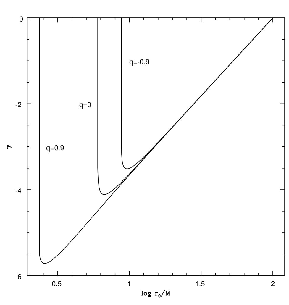
FIG. 3.: Curves showing the change of the orbital eccentricity as the radius $r_{0}$ decreases, in Schwarzschild ($q=0$), and for prograde ($q=0.9$) and retrograde ($q=-0.9$) orbits around a Kerr black hole with $a=0.9M$. In this graph, the parameter $\gamma$ is the natural log of the ratio of the current eccentricity (at $r_{0}$) to the eccentricty the orbit had at $r_{0}=100M$. We can see here clearly that at a certain point (equivalent to the critical radius illustrated in Fig. 1), the eccentricity begins to increase. For an arbitrarily small mass ratio $\mu/M$ it will increase indefinitely before reaching the ISCO, but in any practical case this process will be cut off before too long by the onset of the dynamical instability which causes the orbiting body to plunge inwards toward the central black hole.

REFERENCES

• [1] K. Dansman et al., Lisa Proposal for a Laser-Interferometric Gravitational Wave Detector in Space, Max-Planck-InstitΓΌt fΓΌr Quantenoptik, May, 1993.
• [2] T.A. Apostolatos, D. Kennefick, A. Ori and E. Poisson, Phys. Rev. D 47, 5376 (1993).
• [3] C. Cutler, D. Kennefick and E. Poisson, Phys. Rev. D 50, 3816 (1994).
• [4] T. Tanaka, M. Shibata, M. Sasaki, H. Tagoshi and T. Nakamura, Prog. Theor. Phys. 90, 65 (1993).
• [5] Y. Mino, M. Sasaki, M. Shibata, H. Tagoshi and T. Tanaka, Prog. Theor. Phys. Supl. 128, chapter 1 (1998).
• [6] P.C. Peters, Phys. Rev. 136, B1224 (1964).
• [7] J. Bardeen, Nature 226, 64 (1970).
• [8] D. Kennefick and A. Ori, Phys. Rev. D 53, 4319 (1996).
• [9] F.D. Ryan, Phys. Rev. D 53, 3064 (1996).
• [10] Y. Mino, thesis, Kyoto University, Japan.
• [11] T.C. Quinn and R.M. Wald, Phys. Rev. D 56, 3381 (1997).
• [12] Y. Mino, M. Sasaki and T. Tanaka, Phys. Rev. D 55, 3457 (1997).
• [13] A. Ori, Phys. Lett. A 202, 347 (1995).
• [14] For an analysis of nearly-circular, equatorial orbits of particles in Kerr in post-Newtonian expansion form see H. Tagoshi, Prog. Theor. Phys. 93, 307 (1995).
• [15] C.W. Misner, K.S. Thorne and J.A. Wheeler, Gravitation, pg. 899 (Freeman, New York,1973).
• [16] B. Carter, in General Relativity: An Einstein Centenary Survey, eds. S.W. Hawking and W. Israel (Univ. Press, Cambridge, 1979).
• [17] S. Detweiler, Astrophys. J. 225, 687 (1978).
• [18] R.A. Isaacson, Phys. Rev. 166, 1272 (1968).
• [19] S.A. Teukolsky and W.H. Press, Astrophys. J. 193, 443 (1974).
• [20] S. Chandrasekhar, Proc. Roy. Soc. London A343, 289 (1975).
• [21] M. Sasaki and T. Nakamura, Prog. Theor. Phys. 67, 1788 (1982).
• [22] R.A. Breuer, Gravitational Perturbation Theory and Synchroton Radiation, Lecture Notes in Physics 44 (Springer-Verlag, 1975).
• [23] L.S. Finn, A. Ori and K.S. Thorne, to be published.
• [24] W.H. Press, B.P. Flannery, S.A. Teukolsky and W.T. Vetterling, Numerical Recipes (University Press, Cambridge, 1986).
• [25] J.N. Goldberg, A.J. MacFarlane, E.T. Newman, F. Rohrlich and E.C.G. Sudarshan, J. Math. Phys. 8, 2155 (1967).
• [26] P.M. Morse and H.Feshbach Methods of Theoretical Physics pgs. 1502-1503 (McGraw-Hill, Toronto, 1953).
• [27] M. Shibata, Phys. Rev. D 48, 663 (1993).
• [28] F.D. Ryan, Phys. Rev. D 52, R3159 (1995).