The Singularity in Generic Gravitational Collapse Is Spacelike, Local, and Oscillatory

Abstract

A longstanding conjecture by Belinskii, Khalatnikov, and Lifshitz that the singularity in generic gravitational collapse is spacelike, local, and oscillatory is explored analytically and numerically in spatially inhomogeneous cosmological spacetimes. With a convenient choice of variables, it can be seen analytically how nonlinear terms in Einstein’s equations control the approach to the singularity and cause oscillatory behavior. The analytic picture requires the drastic assumption that each spatial point evolves toward the singularity as an independent spatially homogeneous universe. In every case, detailed numerical simulations of the full Einstein evolution equations support this assumption.

98.80.Dr, 04.20.J

Introduction. Even though much of the theoretical effort in gravitational physics is focused on either quantum gravity or astrophysical sources of gravitational waves, the most fundamental properties of general solutions to Einstein’s equations remain unknown. Foremost among these is the nature of the singularity that forms in generic gravitational collapse. Powerful theorems due to Penrose and Hawking and others [10, 19] predict that some kind of singular behavior will result. However, the proofs of these theorems require very little of the details of the field equations and are thus unable to provide details of the nature of the singularity. Many different types of singular behavior arise in a variety of special cases, but which, if any, of these characterize generic collapse is not known. In fact, it is hard to see that one could hope to answer the question. Einstein’s equations are second order nonlinear partial differential equations (PDE’s) in $3+1$ spacetime dimensions for the metric variables restricted by four constraints and with the freedom to impose four coordinate conditions. It is by no means clear that numerical relativity can help to answer this question either since a code will “blow up” if any variables become singular.

The surprising message of this essay then is that progress in understanding singularities in generic gravitational collapse can indeed be made. It requires a judicious choice of variables and a synergy between numerical simulations which suggest the patterns and analytic predictions which guide the simulations. Our conclusions are based on the properties of solutions with one or two directions of spatial symmetry. While these are not the most general solutions of Einstein’s equations, we believe they are sufficiently generic and sufficiently consistent with each other to indicate how completely general solutions are likely to behave.

Approximately thirty years ago, Belinskii, Khalatnikov, and Lifshitz (BKL) [1] proposed, based on a perturbative analysis, that the singularity in generic collapse was spacelike, local, and oscillatory. In their picture, each spatial point evolves toward the singularity as a distinct Mixmaster universe. Their claim has been criticized but never unambiguously proven or refuted. In addition substantial effort is required to follow their arguments. Our recent work, however, substantially supports their predictions and suggests a simple scenario: It appears that, despite their complexity, Einstein’s equations in the approach to the singularity have an attractor which is dominated by nonlinear terms acting as effective potentials for the dynamics. These potential terms act primarily on one of the gravitational field degrees of freedom and lead to a generic asymptotic solution that supports the BKL description of the generic singularity as spacelike, local, and oscillatory. Other information, such as spatial dependence and the behavior of the other degrees of freedom, is carried along by the dominant behavior.

Our method of studying a given family of solutions as they approach the singualrity is essentially the following [8]: We first determine the velocity-term dominated (VTD) solutions corresponding to the family. These are solutions of the ODE’s which result from the truncation of Einstein’s equations to eliminate all terms containing spatial derivatives (plus certain others; see [12]). Note that the VTD solutions are parametrized by spatially-dependent constants of integration (the “VTD parameters”). We then substitute these solutions into the Einstein equations or into the corresponding Hamiltonian. If, for generic VTD parameters, the terms in the equations or the Hamiltonian containing spatial derivatives become exponentially small (hence, dynamically irrelevant) as $\tau\to\infty$ ($\tau=\infty$ is the time of the spacelike singularity), then we predict that the family is asymptotically velocity-term dominated (AVTD) in the sense that a generic solution of the Einstein equations asymptotically approaches a VTD solution. If not, we monitor which terms might become important (as a result of exponential growth), and we try to predict the subsequent behavior.

We have applied this “Method of Consistent Potentials” (MCP) to various families of cosmological solutions such as the Gowdy spacetimes [7, 16], the Gowdy spacetimes with magnetic fields [20], and $U(1)$ symmetric spacetimes [17, 6]. In all cases, using a choice of time based on geometric invariants connected with the symmetry, we get a clear prediction: either that the spacetime solutions in the family are AVTD, or that they have oscillatory behavior characterized by a sequence of AVTD-like epochs punctuated by “bounces” which involve the short-term awakening of certain of the “potential” terms. Moreover, numerical simulations of solutions of the full Einstein equations (for each family) have in all cases agreed (at generic spatial points) with the MCP predictions. While these numerical simulations cannot be followed all the way to the singularity, they can be taken sufficiently far, with sufficient accuracy, to verify the simple BKL scenario.

We shall now discuss some of the details of these studies, starting with a look at spatially homogeneous cosmologies.

Homogeneous cosmologies. For a spatially homogeneous cosmology with flat spacelike hypersurfaces (Bianchi I), the Hamiltonian for Einstein’s theory takes the form

$$H=-p_{\Omega}^{2}+p_{+}^{2}+p_{-}^{2}=0,$$ (1)

where $p_{\Omega}$, $p_{\pm}$ are respectively canonically conjugate to $\Omega$, the logarithm of the isotropic scale factor, and $\beta_{\pm}$, the (logarithmic) anisotropic shears, and we have the Kasner solutions [13]. These are parametrized by the constants $v_{\pm}=p_{\pm}/|p_{\Omega}|$. Asymptotically ($\Omega\to-\infty$), the shear satisfies

$$\beta_{\pm}=-v_{\pm}\Omega$$ (2)

with $v_{\pm}$ satisfying as a consequence of the constraint (1)

$$v_{+}^{2}\,+\,v_{-}^{2}=1.$$ (3)

For more general homogeneous cosmologies, the Hamiltonian $H$ adds a term $V(\Omega,\beta_{\pm})$ which in certain cases [18] takes the form

$$V(\Omega,\beta_{\pm})=c_{1}e^{a_{1}(\Omega-2\beta_{+})}+c_{2}e^{a_{2}(\Omega+\beta_{+}+\sqrt{3}\beta_{-})}+c_{3}e^{a_{3}(\Omega+\beta_{+}-\sqrt{3}\beta_{-})}+\ \dots\ \ ,$$ (4)

where $c_{i}$ and $a_{i}$ are positive constants. The solutions corresponding to $H$ with this form of the potential are the well-studied Mixmaster solutions [1, 15, 11]. To see the oscillatory behavior of Mixmaster solutions from the MCP point of view, we note that the Bianchi I Hamiltonian (1) is exactly the VTD version of the Mixmaster Hamiltonian, and the VTD solutions are the Kasner spacetimes. If we now substitute these Kasner solutions into (4), as $\Omega\to-\infty$ we have

$$V\to c_{1}e^{a_{1}|\Omega|(-1-2v_{+})}+c_{2}e^{a_{2}|\Omega|(-1+v_{+}+\sqrt{3}v_{-})}+c_{3}e^{a_{3}|\Omega|(-1+v_{+}-\sqrt{3}v_{-})}\equiv V_{1}+V_{2}+V_{3}.$$ (5)

A few moments of reflection will show that the restriction (3) implies that any generic values of $v_{\pm}$ will cause one of the $V_{j}$ to grow and the others to decay. The growing term provides an exponential potential for the dynamics. A bounce off the potential changes the sign of the appropriate combination of momenta. What happens then is that a pattern of growing and decaying terms continues indefinitely. It has long been known that this picture is borne out by the full solutions to Einstein’s equations [1, 4]. An example showing the evolution of the $V$’s and $\beta_{+}$ vs $|\Omega|$ is given in Fig. 1.

Inhomogeneous cosmologies. We first consider the Gowdy family of spacetimes on $T^{3}\times R$. These allow spatial dependence in one direction with periodic boundary conditions and are described in terms of [7, 16, 20] $P(\theta,\tau)$, $Q(\theta,\tau)$, essentially the $+$ and $\times$ polarizations of gravitational waves, and a background $\lambda(\theta,\tau)$. This model has the nice feature that the dynamical equations for the wave amplitudes $P$, $Q$ decouple from the constraints which yield $\lambda$ as a function of the wave amplitudes.

Einstein’s evolution equations are obtained from the Hamiltonian density [16, 20]

$${\cal H}={1\over{4\pi_{\lambda}}}\left({\pi_{P}^{2}+e^{-2P}\pi_{Q}^{2}+e^{-2\tau}P^{\prime 2}+e^{2(P-\tau)}Q^{\prime 2}}\right)$$ (6)

where the $\pi$’s are the conjugate momenta and ${}^{\prime}=\partial/\partial\theta$. The Hamiltonian constraint is the equation for $\dot{\lambda}$ (where the overdot means $\partial/\partial\tau$) while the momentum constraint is one for $\lambda^{\prime}$. Neglecting spatial derivatives in the evolution equations yields, in the limit $\tau\to\infty$, the VTD solution

$$P=v(\theta)\tau,\quad Q=Q_{0}(\theta),\quad\lambda=-v^{2}(\theta)\tau,$$ (7)

with all the momenta dependent only on $\theta$ and $v=\pi_{P}\,/\,2\pi_{\lambda}$. Substitution in (6) shows that the only terms in ${\cal H}$ which could fail to be exponentially small are

$$V_{1}=\left({{\pi_{Q}}^{2}\over{4\pi_{\lambda}}}\right)\,e^{-2P}\to\left({{\pi_{Q}^{0}}^{2}\over{4\pi_{\lambda}^{0}}}\right)\,e^{-2v\tau},\quad V_{2}=\left({{{Q^{\prime}}^{2}}\over{4\pi_{\lambda}}}\right)\,e^{2(P-\tau)}\to\left({{{Q^{\prime}_{0}}^{2}}\over{4\pi_{\lambda}^{0}}}\right)\,e^{2(v-1)\tau}.$$ (8)

$V_{1}$ will grow exponentially if $v<0$. $V_{2}$ will grow if $v>1$. Bounces off $V_{1}$ and $V_{2}$ eventually drive $v$ into the range $0<v<1$, yielding a consistent AVTD solution at almost every spatial point [5, 3]. Fig. 2 shows how this process works for $V_{1}$ and $V_{2}$ and $P$ vs $\tau$ at a typical spatial point.

The “magnetic Gowdy” model is obtained by a change of topology and the addition of a magnetic field [20]. The VTD solution (7) is unchanged. The Hamiltonian (6) picks up an additional term

$$V_{3}=4\,\pi_{\lambda}\,B^{2}\,e^{(\lambda+\tau)/2}$$ (9)

where the constant $B$ measures the strength of the magnetic field and $\lambda$ is now dynamical. Substitution of the VTD solution (7) into (9) yields as $\tau\to\infty$

$$V_{3}=4\,\pi_{\lambda}^{0}\,B^{2}\,e^{(1-v^{2})\tau/2}.$$ (10)

The range $0<v<1$ which allows $V_{1}$ and $V_{2}$ to become exponentially small causes $V_{3}$ to grow. Thus, in the MCP picture, no value of $v$ leads to AVTD behavior. Further MCP qualitative study [20] indicates that at each spatial point, $V_{1}$, $V_{2}$, and $V_{3}$ alternately awaken, causing bounces characteristic of local Mixmaster behavior. Numerical simulations support this prediction with typical behavior shown in Fig. 3.

It is possible to generalize the plane symmetric Gowdy model on $T^{3}\times R$ by removing one of the Killing vectors. This yields vacuum $U(1)$ symmetric models [17, 5, 6]. Here, the dynamical degrees of freedom, now called $\varphi$ and $\omega$, no longer decouple from the background described by $\Lambda$, $z$, and $x$. Einstein evolution equations may be obtained from the variation of ($,_{a}=\partial/\partial x^{a}$ with spatial coordinates $u$, $v$, and time $\tau$)

$$H = \int\int du\kern 1.0ptdv\left({1\over 8}p_{z}^{2}+{1\over 2}e^{4z}p_{x}^{2}+{1\over 8}p_{\varphi}^{2}+{1\over 2}e^{4\varphi}p_{\omega}^{2}-{1\over 2}p_{\Lambda}^{2}+2p_{\Lambda}\right)$$ (13)

$$+e^{-2\tau}\int\int du\kern 1.0ptdv\left\{\left({e^{\Lambda}e^{ab}}\right),_{ab}-\left({e^{\Lambda}e^{ab}}\right),_{a}\Lambda,_{b}+e^{\Lambda}\right.\left[\left({e^{-2z}}\right),_{u}x,_{v}-\left({e^{-2z}}\right),_{v}x,_{u}\right]$$

$$\left.+2e^{\Lambda}e^{ab}\varphi,_{a}\varphi,_{b}+{1\over 2}e^{\Lambda}e^{-4\varphi}e^{ab}\omega,_{a}\omega,_{b}\right\}$$

$$= \int\int du\kern 1.0ptdv\,({\cal H}+2p_{\Lambda})$$ (14)

where $p_{\zeta}$ is canonically conjugate to $\zeta$, $e_{ab}(z,x)$ is the conformal metric in the $u$-$v$ plane, and ${\cal H}=0$ is the Hamiltonian constraint. The choice $p_{\Lambda}>0$ defines the collapsing direction [6]. The VTD solution as $\tau\to\infty$ is

$$z=-v_{z}\tau,\ \ x=x_{0},\ \ \Lambda=(2-p_{\Lambda}^{0})\tau,\ \ \varphi=-v_{\varphi}\tau,\ \ \omega=\omega_{0},$$ (15)

where $v_{z}$, $x_{0}$, $p_{\Lambda}^{0}$, $v_{\varphi}$, $\omega_{0}$, and the remaining momenta are functions of $u$ and $v$ but constants in $\tau$. Upon substitution of the VTD solution (15) into (13), it is seen immediately that the Gowdy-like potential terms

$$V_{z}={\textstyle{1\over 2}}\,p_{x}^{2}\,e^{4z}\to{\textstyle{1\over 2}}\,p_{x}^{2}\,e^{-4v_{z}\tau},\quad V_{1}={\textstyle{1\over 2}}\,p_{\omega}^{2}\,e^{4\varphi}\to{\textstyle{1\over 2}}\,p_{\omega}^{2}\,e^{-4v_{\varphi}\tau}$$ (16)

become negligible if $v_{z}>0$, $v_{\varphi}>0$, as in Gowdy. The very complicated terms in (13) with spatial derivatives have a simple exponential behavior. Given $v_{z}>0$, the inverse conformal metric $e^{ab}$ is dominated by $e^{-2z}$. Examination of the terms in (13) shows that all but one of them have the exponential factor

$$e^{(-2\tau+\Lambda-2z)}\approx e^{(-p_{\Lambda}^{0}+2v_{z})\tau}.$$ (17)

The remaining term is

$$V_{2}={\textstyle{1\over 2}}e^{-2\tau+\Lambda}e^{ab}\omega,_{a}\omega_{b}\approx F(x,\nabla\omega)e^{(-p_{\Lambda}^{0}+2v_{z}+4v_{\varphi})\tau}.$$ (18)

Now as $\tau\to\infty$, the Hamiltonian constraint, with the VTD solution substituted in, becomes

$${\cal H}\approx-{\textstyle{1\over 2}}(p_{\Lambda}^{0})^{2}+2v_{z}^{2}+2v_{\varphi}^{2}\approx 0.$$ (19)

This restriction means that $p_{\Lambda}^{0}>2v_{z}$ so that $p_{\Lambda}^{0},\ p_{z}>0$ implies the exponential decay of terms with the behavior of (17). On the other hand, $V_{2}$ will decay exponentially only if $(p_{\Lambda}^{0})^{2}>(2v_{z}+4v_{\varphi})^{2}$ which is inconsistent with (19). Thus $V_{2}$ must increase exponentially if $v_{z}$ and $v_{\varphi}$ are positive. The Hamiltonian constraint restriction means that $V_{2}$ will grow approximately as $e^{4v_{\varphi}\tau}$ so that $V_{2}$ will act as a potential for the $\varphi$ degree of freedom. A bounce will yield $v_{\varphi}<0$ which will cause $V_{1}$ from (16) to grow exponentially. A bounce off $V_{1}$ will cause the cycle to repeat. All other variables will remain consistent with the VTD solution. Surprisingly, this extremely simple picture describes the results of numerical simulations of the full $U(1)$ symmetric model Einstein equations [21]. The behavior of $V_{1}$, $V_{2}$, and $\varphi$ vs $\tau$ at a typical spatial point is shown in Fig. 4.

Conclusions. The asymptotic approach to the singularity of a sequence of increasingly complicated cosmological spacetimes has been examined. The VTD solution is substituted into the relevant Hamiltonian to obtain a prediction as to whether terms not present in the VTD solution become exponentially small. In the homogeneous Mixmaster case, we find that no matter what the value of the VTD constants, one of three dominant exponential potential terms will always grow. In the vacuum Gowdy case, there are two such potentials at every spatial point and a window, $0<v(\theta)<1$, consistent with AVTD behavior. Addition of a magnetic field (with a suitable change of topology) removes this window and causes the system to oscillate indefinitely as the three potentials grow and decay. Detailed study shows this to be truly local Mixmaster behavior [20]. On the other hand, generic $U(1)$ symmetric models have oscillations between two rather than three potentials at every spatial point although no value of $v_{\varphi}(u,v)$ is consistent with the AVTD solution.

We emphasize that, in the inhomogeneous case, this simplified picture follows from the MCP analysis if the time dependences of a variety of spatially dependent functions are assumed to be negligible compared to the exponentials we have singled out. In every case, this drastic assumption holds true in numerical simulations of the full Einstein evolution equations. This means that we could evolve toward the singularity using ODE’s at every spatial point rather than PDE’s. Thus the BKL conjecture that the generic approach to the singularity is local is very strongly supported. However, it is not yet clear whether, generically, the further conjecture that our observed oscillations are Mixmaster is also correct.

For the inhomogeneous models, the local nature of the dynamics is plausible. It is easy to show that the horizon size goes to zero as $\tau\to\infty$ in both the Gowdy [2] and $U(1)$ cases. Thus, in the chosen time coordinate, the spatial points causally decouple. Information from other sites, carried through the spatial derivatives, ceases to propagate.

There are several implications of these results. First, the local nature of the approach to the singularity means that our choice of cosmological boundary conditions is merely a convenience. The indicated behavior should arise asymptotically in any generic collapse leading to a spacelike singularity. Second, as bounces occur at different spatial points at different times, the amount of spatial structure in the gravitational waves will increase [14, 3]. Third, these results are certainly consistent with a generic spacelike singularity (at $\tau=\infty$) although this was not known before these studies to be a property of $U(1)$ symmetric models.

The simplicity of our picture despite the generality of the one Killing field spacetimes suggests that further generalization is possible. Within the models discussed here, one may for example introduce a scalar field of the type known to suppress Mixmaster oscillations in the homogeneous case [9]. Implementation of the MCP analysis leads in all classes of inhomogeneous models studied here to the prediction that the oscillations will be suppressed. These predictions have not yet been checked by numerical simulation.

Finally, the generalization to the zero Killing field case may be within reach. While precise, quantitative numerical studies in $2+1$ and $3+1$ dimensions must still come to terms with numerical difficulties caused by the spiky features seen in the Gowdy models [5, 3], the local nature of the collapse means that the qualitative features can be seen even at coarse spatial resolutions.

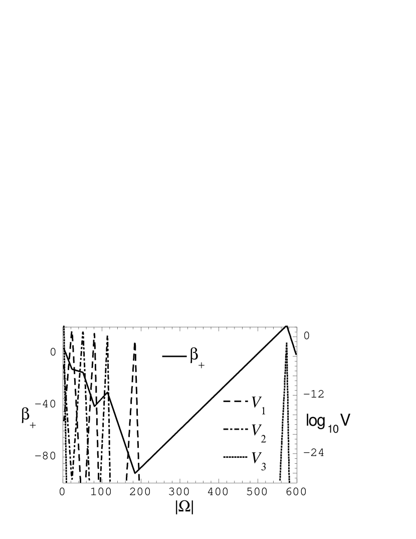
FIG. 1.: A typical Mixmaster trajectory (vacuum Bianchi IX) from a numerical simulation of Einstein’s equations. The potentials $V_{j}$ are defined in (4).

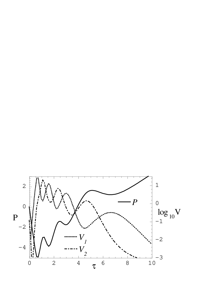
FIG. 2.: Evolution at a representative spatial point in a numerical simulation of Einstein’s equations for a typical vacuum Gowdy model. The potentials $V_{1}$ and $V_{2}$ are defined in (8).

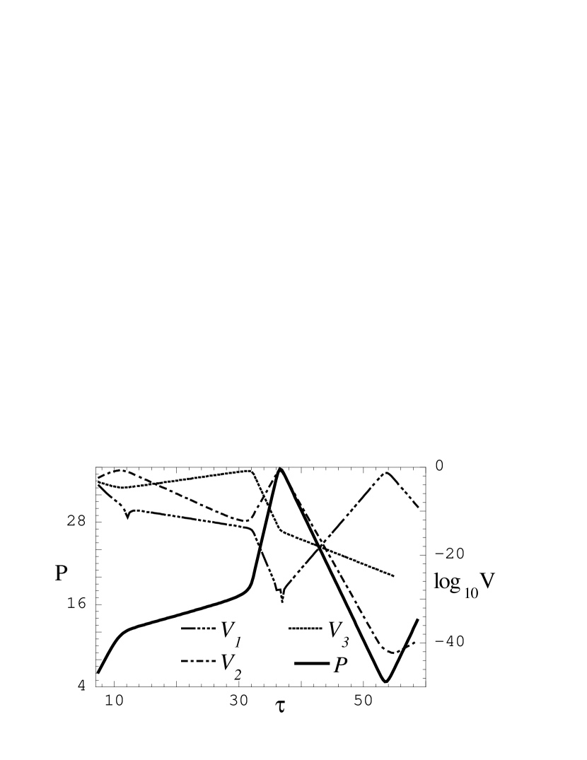
FIG. 3.: Evolution at a representative spatial point in a numerical simulation of Einstein’s equations for a typical magnetic Gowdy model. The potentials $V_{1}$ and $V_{2}$ are defined in (8) while $V_{3}$ is defined in (9).

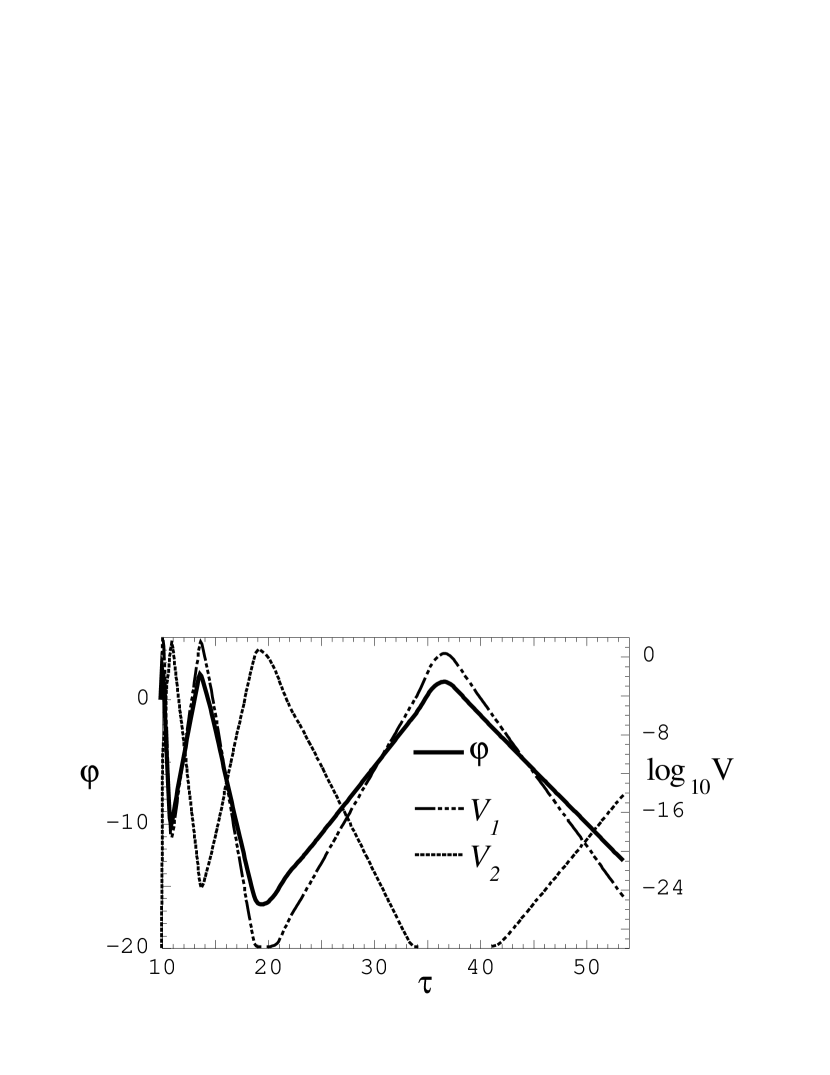
FIG. 4.: Evolution at a representative spatial point in a numerical simulation of Einstein’s equations for a typical generic $U(1)$ symmetric model. The potentials are defined in (16) and (18).

REFERENCES

- [1] Belinskii, V. A., Lifshitz, E. M., and Khalatnikov, I. M., Sov. Phys. Usp.,13, 745–765, (1971).
- [2] Berger, B. K., Ann. Phys. (N.Y.), 83, 458, (1974).
- [3] Berger, B. K., and Garfinkle, D., Phys. Rev. D, 57, 4767 (1998).
- [4] Berger, B. K., Garfinkle, D., and Strasser, E., Class. Quantum Grav., 14, L29–L36, (1997).
- [5] Berger, B. K., and Moncrief, V., Phys. Rev. D, 48, 4676, (1993).
- [6] Berger, B. K. and Moncrief, V., Phys. Rev. D, bf 57, 15 June 1998.
- [7] Gowdy, R. H., Phys. Rev. Lett., 27, 826, (1971).
- [8] Grubis̆ić, B., and Moncrief, V., Phys. Rev. D, 47, 2371–2382, (1993).
- [9] Halpern, P., J. Gen. Rel. Grav., 19, 73–94, (1987).
- [10] Hawking, S. W., and Penrose, R., Proc. Roy. Soc. Lond. A, 314, 529–548, (1970).
- [11] Hobill, D., Burd, A., and Coley, A., eds., Deterministic Chaos in General Relativity, (Plenum, New York, 1994).
- [12] Isenberg, J. A., and Moncrief, V., Ann. Phys. (N.Y.), 199, 84, (1990).
- [13] Kasner, E., Trans. Am. Math. Soc., 27, 155–162, (1925).
- [14] Kirillov, A. A., and Kochnev, A. A., JETP Lett., 46, 435–438, (1987).
- [15] Misner, C. W., Phys. Rev. Lett., 22, 1071–1074, (1969).
- [16] Moncrief, V., Ann. Phys. (N.Y.), 132, 87–107, (1981).
- [17] Moncrief, V., Ann. Phys. (N.Y.), 167, 118, (1986).
- [18] Ryan, Jr., M. P., and Shepley, L. C., Homogeneous Relativistic Cosmologies, (Princeton University, Princeton, 1975).
- [19] Wald, R. M., General Relativity, (University of Chicago Press, Chicago, 1984).
- [20] Weaver, M., Isenberg, J., and Berger, B. K., Phys. Rev. Lett., 80, 2984 (1998).
- [21] Berger, B. K. and Moncrief, V., submitted to Phys. Rev. D, gr-qc/9804085.