a Manuela

ai miei genitori

Ringraziamenti

Desidero ringraziare il mio supervisore prof. Sergio Zerbini per avermi dato la possibilità di studiare gli interessanti argomenti che sono oggetto di questa tesi, per le numerose discussioni ed utili consigli.

Vorrei inoltre ringraziare il mio collega e coautore dr. Valter Moretti per la sua collaborazione fondamentale per ottenere molti dei risultati esposti in questa tesi.

Sono grato al mio controrelatore prof. Emilio Elizalde per i suggerimenti e le critiche costruttive.

Ci sono numerose altre persone che vorrei ringraziare, in particolare il dr. Guido Cognola, il prof. Ruggero Ferrari, il dr. Dimitri V. Fursaev, il dr. Edisom S. Moreira Jnr., il dr. Giuseppe Nardelli, il prof. Marco Toller, il dr. Luciano Vanzo e il dr. Andrei Zelnikov. Altri ringraziamenti per alcuni suggerimenti specifici si trovano in fondo ai lavori pubblicati.

Infine, vorrei ringraziare i miei compagni del X ciclo di dottorato Stefano Dusini, Riccardo Giannitrapani e Franco Toninato per questi tre anni irripetibili.

Prefazione

Questa tesi tratta di alcuni aspetti della teoria quantistica dei campi su spazi che contengono singolarità di tipo conico, con particolare riferimento al caso della stringa cosmica, della teoria a temperatura finita nello spazio di Rindler e vicino all’orizzonte di un buco nero di Schwarzschild.

La tesi riassume i risultati ottenuti durante gli ultimi due anni del corso di Dottorato di Ricerca, sia già pubblicati in alcuni articoli che del materiale inedito. I lavori pubblicati, o comunque accettati per la pubblicazione al momento della stesura della presente tesi, corrispondono alla bibliografia [100, 101, 118, 99, 102].

Il lavoro è organizzato nel modo seguente. Dopo un’introduzione generale, il Capitolo 1 ha carattere introduttivo alla singolarità conica e alle tecniche di regolarizzazione basate sul nucleo del calore e la funzione $\zeta$. Il Capitolo 2, basato su [102], ha interesse generale per la teoria quantistica dei campi sugli spazi curvi, introducendo un nuovo metodo per la regolarizzazione delle fluttuazioni del vuoto usando la funzione $\zeta$. Nel Capitolo 3, basato su [99], viene esteso il metodo della funzione $\zeta$ sul cono al caso di un campo con massa. Il risultato ottenuto viene poi usato per calcolare il tensore energia-impulso, le fluttuazioni del campo e la contro-reazione delle fluttuazioni quantistiche sulla metrica di una stringa cosmica. Il Capitolo 4, che contiene la maggior parte del materiale inedito, tratta del calcolo delle correzioni quantistiche all’entropia di Bekenstein-Hawking usando il metodo della singolarità conica. Nel Capitolo 5, basato su [100, 101], viene esteso il metodo della singolarità conica al caso del campo del fotone e del gravitone, risolvendo alcuni problemi non banali legati all’invarianza di gauge. Nel Capitolo 6, che è una rielaborazione di [118] con dei contributi inediti, la teoria del campi sullo spazio conico viene studiata usando il metodo della trasformazione conforme alla metrica ottica, sia per il campo scalare che per il campo elettromagnetico, mettendo in evidenza alcuni problemi della teoria termica nello spazio conico. Infine, nelle conclusioni vengono sottolineati i principali problemi aperti della teoria sul cono e degli altri argomenti trattati.

La tesi è scritta in inglese. A questo proposito vorrei ringraziare il Ministero dell’Università e della Ricerca Scientifica e Tecnologica per aver finalmente dato la possibiltà di scrivere le tesi di dottorato in lingue diverse dall’italiano, favorendo in questo modo lo scambio dell’informazione nella comunità scientifica e l’utilità stessa della tesi a livello internazionale.

Introduction

The aim of this thesis is to investigate some aspects of the behaviour of quantum fields propagating in curved or non-trivial spacetimes. The gravitational field, namely the metric of the background, is treated classically, while the matter quantum fields are quantized. This approach is very useful when the interaction between fields and gravity is important, but not the quantum nature of the gravitational field itself. It can be reasonably assumed that non-trivial gravitational effects occur when one considers quantum modes with a wavelength comparable with the characteristic curvature radius of the background spacetime. This approach resembles the semiclassical calculations in the early days of quantum theory, in which the electromagnetic field was considered as a classical background field, interacting with the quantized matter.

Although one cannot expect that this approach gives final answers about unification and quantum gravity, it is very important and appealing because of the results obtained in the past twenty-five years and, in particular, the open problems that has raised. Indeed, in some of the topics faced in QFT in curved spacetimes one touches with the hand the limits of the present theories of gravitation and quantum fields. Furthermore, it is up to now the only way to say something about the influence of the gravitational field on the quantum phenomena.

The Hawking radiation and the Unruh effect are among the most important results of quantum field theory in curved spacetime and provide a beautiful unification of aspects of quantum theory, gravitation, and thermodynamics. Furthermore, the lack of an explanation of the huge entropy of a black hole in terms of statistical mechanics, namely counting the number of possible underlying quantum states, is probably the clearest indication that the present theories are close to their limits. We remind that, in units $c=\hbar=G=k_{B}=1$, a ball of thermal radiation has mass $M\sim T^{4}R^{3}$ and entropy $S\sim T^{3}R^{3}$, $T$ being the temperature and $R$ the radius of the ball. The radiation will form a black hole when $R\sim M$, and so when $T\sim M^{-1/2}$ and $S\sim M^{3/2}$. In contrast, the Bekenstein-Hawking entropy of the resulting black hole is $S_{BH}\sim M^{2}$. Therefore, a black hole with a mass much larger than the Planck mass, $M\gg 1$, has an entropy which is much larger than the entropy of the radiation that formed it. It is worth stressing that the thermal radiation has the highest entropy of ordinary matter. Furthermore, when one tries to compute the entropy of the quantum fluctuations living outside the horizon of a black hole, which can be considered as the first quantum correction to the thermodynamical Bekenstein-Hawking entropy, one finds that it is divergent and some cutoff is needed, such as a ‘fuzzy’ horizon: in the present theory it is difficult to find a satisfactory way to introduce such a cutoff.

All these problems make the black-hole entropy and its quantum corrections a very interesting subject to study. In some sense, there is an analogy with the ultraviolet catastrophe in the black-body radiation, the study of which gave rise to the quantum theory.

Regarding the the problem of the explanation of the microscopical origin of black hole entropy, it has be mentioned that much progress has been done in the last two years in the context of string theory. Indeed, a few years ago Susskind [137] suggested that there should be a one to one correspondence between strings and black holes, and that within this correspondence the enormous black-hole entropy could be explained counting the number of excited string states. Only very recently some apparent contradictions in the correspondence have been resolved, but now within string theory it is possible to reproduce the correct dependence on the mass and charges for essentially all black holes, although only for certain black holes the numerical coefficient of the entropy can be computed and shown to agree (for a recent review see [98][120]). This is clearly a subject of great interest to discuss and which opens new prospects for the understanding of the black hole entropy and related phenomena, but it is outside the reach of this thesis and I am not discussing it here.

Many different methods have been developed for computing the Bekenstein-Hawking entropy and its quantum corrections. Among these, the method of the conical singularity, introduced by Gibbons and Hawking [77], has been proved useful and effective, especially for computing the quantum corrections, but has also produced some contradictory results. As we will see, in order to apply this method it is necessary to employ one-loop physics for quantum fields living on manifolds with conical singularities: indeed, the aim of this thesis is to discuss some aspects of quantum field theory on this kind of manifolds.

The computation of the black-hole entropy is not the only case in which one comes across conical singularities. Another case that I will consider is the spacetime around an idealized cosmic string, whose study can have relevant cosmological applications. Indeed, the Rindler metrics, which one usually considers when computing the black-hole entropy, and the cosmic string metric are closely related, and most of the results obtained for one spacetime can be translated for the other by means of an appropriate identification. Other examples of conical singularities, that will not be discussed in the present thesis, are the orbifolds occurring in string compactification [84], the configuration space of gravitation theory [39] and the quantum gravity in $2+1$-dimensions [141].

Most of the original results exposed in this thesis have been obtained during the years ’96-’97 by myself or by dr. Valter Moretti and myself and published in five papers [100, 101, 118, 99, 102]. The present thesis contains also some new results which have not been published before. In particular, these results concerns the computation of regularized one-loop quantities for massive scalar fields on the cone from the integral representation of the heat kernel, and the relation among local and global approach for the regularization of quantum field theory on the cone. These new results are reported in Chapters 1 and 4.

The thesis is organized as follows. In Chapter I will review some of the techniques that will be used in the following Chapters. After a short introduction to the Rindler space and to the cosmic string, I will review the one-loop regularization of the effective action, with particular care for the $\zeta$-function regularization. Then I will discuss the possibility of regularizing the conical manifold by means of smooth manifolds which approximate it. It will be shown that this procedure is reliable only in the limit of vanishing deficit angles. Anyway, the smoothed singularity has the advantage of allowing the use of standard Riemannian geometry and is useful to gain some understanding of the conical geometry. In the subsequent two sections I will review the computation of the heat kernel and the $\zeta$ function of the Laplace-Beltrami operator on the flat cone, which will be the main tools used throughout the thesis for computing one-loop effects. In the final subsection I will introduce a new procedure to compute the integrated $\zeta$ function on the cone from the local one. This procedure gives results in agreement with those the integrated heat kernel on the cone and will be useful for clarifying the mysterious relation between local and integrated quantities. This is not a secondary point: it is my opinion that the relation between local and integrated quantities on the cone is the main point which remains to be clarified on quantum field theory on the cone. In Chapter 4 I will argue that the local approach is physically more reasonable, but many authors still use the integrated approach and the question has not been settled down yet.

Chapter 2 has a general character and it is essentially based on [102]. Here a new prescription is introduced for computing the vacuum fluctuations $\langle\phi^{2}\rangle$. This prescription, apart for being closer to the general spirit of the $\zeta$ function regularization, has the advantage of not requiring any subtraction of a reference state for defining the fluctuations, a subtraction which is necessary with the usual prescription. The new prescription is then applied to some examples, in particular to the closed static Einstein universe for general coupling and mass. An useful expression for the trace of stress tensor of a non-conformal invariant scalar field is also given.

In Chapter 3 I consider massive fields on the cone. The massive case on the cone was an open problem when I started this thesis: although there were representations for the heat-kernel and the Green functions for massive fields, these were so complicate that only few explicit results were available. Actually, only in [114] some explicit results were given. In paper [99], on which this Chapter is based, the $\zeta$ function for a massive scalar field was finally computed as a power series of $(mr)^{2}$, where $m$ is the mass of the field and $r$ is the proper distance from the apex of the cone. The approximation is the right one for computing quantum effects near a cosmic string or near the horizon of a black hole. By means of the $\zeta$ function it was not only possible to confirm the results of [114], but also compute important quantities such as the effective action and, in particular, the energy-momentum tensor. The results obtained have been recently confirmed by new computations, partially reported in Chapter 4, and based on the heat-kernel technique. Although in this Chapter I mainly focus on the cosmic string case, the results are easily translated for the Rindler case. In the final section of this Chapter I present an interesting application: the energy-momentum tensor of a massive field is employed for computing the back reaction of the quantum fluctuations on the background metric, showing how the conical geometry is changed by quantum effects.

Chapter 4 is devoted to the study of the quantum corrections to the black hole entropy that, as I have said above, is the main motivation for studying quantum field theory on manifold with conical singularities. After a short review of the tree level black hole entropy and the one-loop corrections, I discuss the conical singularity method by comparing the local and integrated approaches, and showing that they give different results. In particular, the horizon divergences in the thermodynamical quantities, expected from simple arguments based on the the behaviour of the local temperature, seem to arise in a completely different way in the two approaches. However, it is shown the the divergences in the integrated approach should be more properly interpreted as usual ultraviolet divergences, and in fact they can be renormalized away by redefining the Newton constant in the standard way, while the horizon divergences are not present in this approach. It is then argued that the local approach, in which the horizon divergences arise in a natural way, is physically more reasonable, although the question has not completely settled down yet. Then, in the last two sections, I briefly discuss the conjecture, due to Susskind and Uglum [138], of a possible renormalization of the horizon divergences in the local approach and the case of a non-minimally coupled field.

In Chapter 5 I discuss the generalization of the local $\zeta$ function on the cone to the case of the Maxwell field and the graviton field. The final result is just what one expects by counting the number of degrees of freedom of the fields, so that, for instance, one sees that the contribution of the photons or of the gravitons to the one-loop quantum corrections to the entropy in the Rindler space is just twice that of the massless scalar field. However, to derive this result one has to deal with the presence in the theory of gauge-dependent terms. These terms arise as surface terms and would disappear on regular manifolds, but remain in the theory because of the conical singularity. Actually, in section 5.2 the presence of such gauge-dependent terms is conjectured on more general manifolds. In [100] it was argued that the gauge-dependent surface terms should be discarded on the conical manifold as would happen on regular manifolds, since this is the only possible procedure to obtain physically reasonable results. In particular, this procedure gives an entropy which not only is independent on the gauge chosen, but is positive for any value of the temperature. If fact, the paper [100], on which this Chapter is based, originated from discussions about an interesting paper by Kabat [105]. In such paper it was shown that the one-loop quantum corrections to the black-hole entropy due to the electromagnetic field could be negative, and this negative entropy was identified with a low-energy relic of string theory effects conjectured by Susskind and Uglum [138]. Kabat’s result was regarded as very interesting in literature, but the negative result in [100] showed that, after all, photons do not remember much about the possible underlying string theory.

In Chapter 6 I discuss the optical approach, both on some aspects of general interest and on the specific case of the Rindler space. In the Introduction to this Chapter I review the relation between the canonical definition of the free energy of a system and the path integral approach, showing that the canonical free energy is equivalent to the path integral formulation in the optical related manifold rather than in the physical manifold. The difference between the free energies computed in the physical manifold and in the optical manifold is the logarithm of the functional Jacobian of the conformal transformation which relates the two manifolds. On regular manifolds this Jacobian changes only the value of the zero-temperature energy, which does not affect the thermodynamics. On the conical manifold the question more subtle, since the conical singularity could introduce a less trivial dependence on the temperature: in four dimension no explicit computation has been possible yet, and this issue, discussed in Appendix B, is still under investigation. In section 6.1 the results of the optical results and the results obtained in Chapter 4 in the physical static manifold are compared in the case of a scalar field: although the term proportional to $T^{4}$ agrees, the results differ for the coefficient of the term proportional to $T^{2}$, and the reason for this difference is still obscure. Furthermore, it is shown that there are some inconsistencies in the statistical-mechanical relations if one employs the one-loop quantities computed in the physical static manifold, while no such inconsistencies appear for the optical results. In any case, these problems have no direct influence on the discussion on the quantum corrections to the entropy of a black hole done in Chapter 4. In sections 6.2 the optical approach is extended to the case of the electromagnetic field, and in section 6.3 this approach is applied to the particular case of the Rindler space. Here an important result is that the gauge-dependent terms in the effective action, analogous to those encountered in Chapter 5, are canceled out by the ghost fields, and so the gauge-invariance is restored in a more satisfactory way. The free energies of the gas of photons computed with the direct and the optical methods are compared, and the conclusions are similar to those for the scalar fields.

To finish with, I would like to comment about the bibliography. I have tried to do my best to acknowledge the importance and the priority of each article. However, the number of papers is so large that probably I have not succeeded completely. Therefore, I would like to beg the pardon form all the authors that I have forgot or not considered with the right weight.

In this thesis I will use units such that $c=\hbar=G=k_{B}=1$. However, in order to stress some physical fact, in some case I will write explicitly the relevant constants.

Chapter 1 On the conical space

Introduction

In this first Chapter we review some well-known facts and tools that we will use throughout the thesis.

In the next two sections we start introducing and discussing some basic facts about two well-known spacetimes which show conical singularities, namely the Rindler wedge and the space around a cosmic string. Actually, as we will see, while the cosmic string background shows the conical singularity also in the Lorentzian section, in the Rindler space the singularity appears only when one considers the finite-temperature theory within the periodic Euclidean time formalism.

In section 1.3 we review the heat-kernel and the $\zeta$-function regularizations of the one-loop quantum field theory on a general curved manifold. We also discuss the relation among different regularization procedures, an important topic that will be used in Chapter 4.

The last three sections are devoted to conical space. In section 1.4 we discuss the Riemannian geometry of the cone by approximating it by means non-singular manifolds. In this way it is possible to understand some interesting facts about the cone geometry, but the results must be used with care since, as we will see, they are correct only for small deficit angles. In section 1.5 we will review the computation of the heat kernel for the Laplace-Beltrami operator on the cone, a subject which has a very long story initiated in the last century by the works of Sommerfeld. Finally, in the last section we will review the computation of the local $\zeta$ function on the cone. There we give also some new results about the tricky relation among local and integrated quantities on the cone.

1.1 A short introduction to the Rindler space

Finite temperature field theory in the Rindler wedge will be the main subject of this thesis and, therefore, we start by reminding some definitions and some basic facts about the Rindler wedge. Since this space has been discussed in details in thousands of beautiful papers and reviews, we refer to them for a deeper discussion (see, for instance, [143, 68, 15, 142, 150]).

The Rindler wedge is a submanifold of the Minkowski spacetime which can be considered as the part of Minkowski spacetime causally accessible to an accelerated observer. Let us consider the $D$-dimensional Minkowski spacetime with Cartesian coordinates $(t,x,{\bf x}_{\perp})$ and line element

$$ds^{2} = -dt^{2}+dx^{2}+d{\bf x}_{\perp}^{2}.$$

Consider then the Rindler coordinates $(\tau,r)$ in place of $(t,x)$:

$$x = r\,\mbox{cosh }\tau,$$

$$t = r\,\mbox{sinh }\tau,$$ (1.1)

with $0<r<+\infty$ and $-\infty<\tau<\infty$. This can be seen as the Minkowskian version of the transformation from Cartesian to cylindrical coordinates in Euclidean space. Then the line element takes the form

$$ds^{2} = -r^{2}\,d\tau^{2}+dr^{2}+d{\bf x}_{\perp}^{2}.$$ (1.2)

The above Rindler metric is static but not ultrastatic. Clearly, the Rindler coordinates do not cover the whole Minkowski spacetime, but only what is called the right Rindler wedge $W_{R}$: $x>|t|$. One could also consider the left Rindler wedge $W_{L}$, $x<-|t|$, which can be obtained by reflecting $W_{R}$ by means of the transformation $(t,x,{\bf x}_{\perp})\rightarrow(-t,-x,{\bf x}_{\perp})$. For sake of brevity, by Rindler wedge we will always mean the right wedge.

The components of the metric in the Rindler coordinates do not depend on $\tau$, and so $\partial_{\tau}$ is a time-like Killing vector: in Cartesian coordinates it is written as $x\partial_{t}+t\partial_{x}$, showing that the symmetry related to $\partial_{\tau}$, $\tau\rightarrow\tau+\tau_{0}$, has the character of a boost rather than of an ordinary time translation. Furthermore, the Rindler wedge is a globally hyperbolic manifold [69] in the sense that the Cauchy problem is well posed assigning the initial data on a surface of constant $\tau$, and so field theory is well founded in $W_{R}$.

Consider now a world line such that

$$r(\eta) = \mbox{constant}=a^{-1},$$

$${\bf x}_{\perp}(\eta) = \mbox{constant},$$

where $\eta$ is the proper time along the world line. From the line element follows that $\tau(\eta)=a\eta$ and in the Minkowski coordinates this world line takes the form

$$t(\eta) = a^{-1}\mbox{ sinh }a\eta,$$

$$x(\eta) = a^{-1}\mbox{ cosh }a\eta,$$

$${\bf x}_{\perp}(\eta) = \mbox{constant},$$

which is the world line of an observer who is accelerating uniformly with respect to the proper time $\eta$ with proper acceleration $a$. Notice that the hypersurfaces with constant $r$ are hyperbolae asymptotic to the hypersurfaces $t=\pm x$.

The two null hypersurfaces $t=\pm x$ form a bifurcate Killing horizon for a Rindler observer: the hypersurface $t=-x$ is a past horizon which divides the Rindler observers from the region of Minkowski spacetime in which they cannot send information, and the future horizon $t=x$ divides them from the region from which they cannot receive information.

It is important to notice that the Rindler metric is an approximation of the metric of the region near the horizon of a Schwarzschild black hole, as we will see in Chapter 4. Physically this is related to the fact that an observer at rest in the static gravitational field outside the horizon of the black hole must undergo a constant acceleration to avoid being pulled into the horizon: this situation is physically close to the flat space as experienced by an accelerated observer as the Rindler ones.

Passing to the Euclidean section, namely analytically continuing the Rindler metric to imaginary values of the Rindler time, $\tau\rightarrow i\tau$, we obtain the line element

$$ds^{2} = r^{2}\,d\tau^{2}+dr^{2}+d{\bf x}_{\perp}^{2}.$$ (1.3)

Particularly interesting is the case when we pass to the Euclidean section for considering a finite temperature field theory: in that case we must also make the imaginary time periodic: $0\leq\tau\leq\beta$ with $\tau=0$ and $\tau=\beta$ identified, where $\beta=T^{-1}$ is the inverse temperature. In doing this the Euclidean Rindler manifold becomes the manifold $C_{\beta}\times R^{D-2}$, where $C_{\beta}$ is the simple two-dimensional flat cone with deficit angle $2\pi-\beta$: the manifold has a conical singularity at $r=0$ unless $\beta=2\pi$.

Let us now remind some important results of quantum field theory in the Rindler wedge. The most important fact, known as Unruh effect [143], is that a Rindler observer experiences the usual Minkowski vacuum as a thermal state with temperature $T=1/2\pi$, the Unruh-Hawking temperature. Notice that this is the only temperature at which the metric (1.3) is non singular and that the local temperature is $T_{L}(x)=1/2\pi r$. This effect can be seen from the Bogolubov coefficients [15] or by comparing the two-point functions [70]. The physical interpretation of this phenomenon can be summarized as follows [139]. In the Minkowski space there are the usual fluctuations of the vacuum. This fluctuations are closed loops in spacetime. Some of these loops will encircle the origin $t=x=0$ of Minkowski spacetime and therefore they lay partially inside and partially outside the Rindler wedge. While a Minkowski observer would not distinguish these fluctuations from the others, as the Rindler observer is concerned they are particles which intersect the past and future horizon, and so are particles present for all time: a Rindler observer sees these fluctuations as a bath of thermal particles which are ejected from the horizon infinitely far in the past and which will eventually fall back onto the horizon in the infinite future. To this bath of thermal particles is associated an entropy which is proportional to the area of the horizon and divergent, as we will see in the next Chapters.

The origin of these thermal states can also be seen in an elegant way as entropy of entanglement [16, 136, 106, 28, 105]. Let us suppose to divide the Cauchy hypersurface at $t=0$ of Minkowski space into two halves, one with $x<0$ and one with $x>0$. Assume then that the Hilbert space ${\cal H}$ on the hypersurface factorizes into a product space ${\cal H}_{L}\otimes{\cal H}_{R}$, with orthonormal basis $|b\rangle_{L}$ and $|a\rangle_{R}$ respectively. Then a general ket $|\psi\rangle$ can be written as

$$|\psi\rangle = \sum_{b,a}\psi(b,a)\,|b\rangle_{L}\otimes|a\rangle_{R}.$$

Since no causal signal from the hypersurface $t=0$, $x<0$ can reach the right Rindler wedge, the complete set of states on the hypersurface $t=0,\,x>0$ is the complete set of states to describe the physics in the Rindler space for all time. Therefore, when we restrict the quantum theory to $W_{R}$ we must trace over the degrees of freedom in ${\cal H}_{L}$ obtaining a density matrix

$$\rho(a,a^{\prime}) = \sum_{b}\psi(b,a)\psi^{\ast}(b,a^{\prime}).$$

This means that a pure state for an inertial observer, such as the Minkowski vacuum, is seen as a thermal state by an accelerated observer.

We will come back to these and other aspects of quantum field theory in the Rindler space in the following Chapters.

1.2 A short introduction to cosmic strings

In this section we summarize very briefly some basic facts about cosmic strings. The main reference here is the report by Vilenkin [146]. Cosmic strings are essentially topological defects of the vacuum of a field which can form when a continuous symmetry is broken during a cooling process. Cosmic strings are of great importance for cosmological models where, for instance, they could act as seeds for galaxy formation. The simplest model that gives rise to cosmic strings is that of a self-interacting complex scalar field $\phi$, for instance the Higgs field, with symmetry group $U(1)$, $\phi\rightarrow e^{i\alpha}\phi$:

$${\cal L} = \partial_{\mu}\phi^{\dagger}\partial^{\mu}\phi-V_{T}(\phi).$$

The self-interaction potential contains a temperature-dependent term, for example

$$V_{T}(\phi) = AT^{2}\phi^{\dagger}\phi+\frac{1}{2}\lambda(\phi^{\dagger}\phi-\eta^{2})^{2},$$

where $\lambda$ is the self-coupling constant and $A>0$ is a dimensionless constant. At temperature $T$ the effective mass of the theory is

$$m^{2}(T) = AT^{2}-\lambda\eta^{2},$$

and so we have the critical temperature $T_{c}=\eta\sqrt{\lambda/A}$ at which the effective mass of the theory is zero and we have a second-order phase transition. For $T>T_{c}$ the effective mass $m^{2}(T)$ is positive and the vacuum expectation value of the field is $\langle\phi\rangle=0$: the symmetry $U(1)$ is restored for $T>T_{c}$. At low temperature, instead, the field acquires a vacuum expectation value $\langle\phi\rangle=\eta e^{i\theta}$, where the phase $\theta$ is arbitrary: the vacuum is degenerate and the symmetry $U(1)$ is broken at low temperature. The arbitrary phase $\theta$ varies in the space and, since $\langle\phi\rangle$ is a single valued function, the total change of $\theta$ around a closed loop must be $\Delta\theta=2\pi n$, where $n$ is an integer. If we consider a closed loop with, e.g., $\Delta\theta=2\pi$ we can continuously shrink it to a point, for which $\Delta\theta=0$, only if we encounter one point for which the phase is undefined, namely $\langle\phi\rangle=0$. The set of such points must form a closed loop or an infinite line, which are called cosmic strings, otherwise it would be possible to contract the loop without crossing a singular point. This shows that at least a cosmic string, namely a tube of false vacuum $\langle\phi\rangle=0$, should exist for any loop with $n\neq 0$.

The radius of the string core is of the order of the Compton wave length of the Higgs boson, $r_{0}\sim m_{\phi}^{-1}=(\eta\sqrt{\lambda})^{-1}$, and the mass per unit length is $\mu\sim\eta^{2}$.

Since for strings of cosmological interest the length is much greater that their width, if we are not interested in the internal structure of the string we can represent its energy-momentum tensor as proportional to a $\delta$-function peaked on the string. For instance, for a static straight string lying along the $z$-axis, Lorentz invariance for boosts along $z$ and the conservation laws fix the energy-momentum tensor to

$$T_{\mu\nu} = \mu\delta(x)\delta(y)\mbox{diag}(1,0,0,-1).$$

The metric of the space around the string is then a solution of the Einstein equations

$$R_{\mu\nu}-\frac{1}{2}g_{\mu\nu}R = 8\pi GT_{\mu\nu}.$$

The solution has been found by several authors [145] and in cylindrical coordinates is

$$ds^{2} = -dt^{2}+dz^{2}+dr^{2}+(1-4G\mu)^{2}r^{2}d\theta^{2},$$ (1.4)

which, in the spatial section $(r,\theta)$ describes a simple flat cone with deficit angle $2\pi-\alpha=8\pi G\mu$. For typical GUT theories the symmetry breaking scale is around $10^{16}GeV$, so that $\mu\sim 10^{-6}$ and $2\pi-\alpha\sim 10^{-6}$. It is clear that the Euclidean version of the above metric is the same as the Euclidean Rindler metric (1.3) after a suitable identification of the coordinates.

It is well known that, even though the space around a infinitely long, static and straight cosmic string is locally flat, the non-trivial topology gives rise to remarkable gravitational and quantum phenomena. For example, the classical trajectories of particles are deviated by the cosmic string by the same (absolute) angle independently of the radius of closest approach (see, e.g., [146, 6]). Moreover, the presence of the string allows effects such as particle-antiparticle pair production by a single photon and bremsstrahlung radiation from charged particles [90, 130] which are not possible in empty Minkowski space, due to conservation of linear momentum. Finally, the string polarizes the vacuum around it, in a way similar to the Casimir effect between two conducting planes forming a wedge [42, 95]: this last effect will be the our main interest in cosmic strings in this thesis.

1.3 Short introduction to $\zeta$ function and heat kernel

The $\zeta$-function and heat-kernel techniques are tools extensively used in this thesis, and therefore in this section we summarize some basic facts about the methods [51, 91, 15, 56, 53, 26].

Let us start considering a matter quantum field $\phi$ living on a $D$-dimensional background manifold ${\cal M}$ with a metric $g_{\mu\nu}$. Moreover, let us suppose that the metric is static, namely $\partial_{0}g_{\mu\nu}=0$ and $g_{0i}=0$, so that it is always possible to perform the analogue of the Wick rotation and make the metric Euclidean. The general case is more subtle and will not be considered in this thesis. The physical properties of the field can then be described by means of the Euclidean path integral [15]

$$Z[g] = \int{\cal D}\phi\,e^{-S_{E}[\phi,g]},$$

where $S_{E}[\phi,g]$ is the classical action of the field and the functional integral is taken over the field configurations satisfying suitable boundary conditions. The functional integration measure is the usual covariant one, ${\cal D}\phi=\prod_{x}d\phi(x)g^{1/4}(x)$. Finally, an infinite renormalization constant has been neglected.

The physical interpretation of the quantity $Z[g]$ is that, if the spacetime is asymptotically flat and the functional integral is taken over fields infinitesimally close to the classical vacuum, then $Z[g]$ is the vacuum to vacuum transition amplitude. Moreover, the quantity $W[g]=-\ln Z[g]$ generates the effective field equations, namely the classical ones plus quantum corrections, and therefore it is called effective action.

When the condition of asymptotically flatness is not satisfied, then the physical meaning of $Z[g]$ is less clear, but the functional $W[g]$ is still supposed to describe the effective action.

The dominant contribution to the path integral $Z[g]$ will come from fields that are near the solution $\phi_{0}$ of the classical field equations, namely which extremizes the action and satisfy the boundary conditions. Therefore, it is possible to expand the action in a Taylor series about the classical solution:

$$S_{E}[\phi,g] = S_{E}^{c}[\phi_{0},g]+S_{E}^{(2)}[{\tilde{\phi}},g]+\mbox{higher order terms in }{\tilde{\phi}},$$

where ${\tilde{\phi}}=\phi-\phi_{0}$ are the fluctuations and $S_{E}^{(2)}[{\tilde{\phi}},g]$ is quadratic in ${\tilde{\phi}}$. The above approximation is sufficient for considering one-loop effects, namely at first order in $\hbar$: the one-loop generating functional, known also as zero-temperature partition function or simply partition function, reads

$$Z[\phi,g] \simeq e^{-S_{E}^{c}[\phi_{0},g]}\int{\cal D}{\tilde{\phi}}\,e^{-\frac{1}{2}S_{E}^{(2)}[{\tilde{\phi}},g]}.$$

For a neutral scalar fields the quadratic terms have the form

$$S_{E}^{(2)}[{\tilde{\phi}},g] = -\frac{1}{2}\int_{M}{\tilde{\phi}}\,A\,{\tilde{\phi}},$$

where $A$ is known as the small disturbance or small fluctuations operator. When the background metric is Euclidean, $A$ is a second order, elliptic, self-adjoint (or with a self-adjoint extension), and non-negative operator. For a quasi-free scalar field, namely that interacts only with the background metric, the operator $A$ reads $A=-\Delta+m^{2}+\xi R$, where $\Delta$ is the Laplace-Beltrami operator on the manifold ${\cal M}$, $m$ is the mass of the field, $R$ is the scalar curvature of the manifold and $\xi$ is an arbitrary constant. If the field is self-interacting, $A$ will depend on the classical solution $\phi_{0}$ and a more sophisticated treatment is needed, especially if $\phi_{0}$ is not a constant configuration. The charged scalar field case is very similar, while in the Dirac’s field case the small disturbance operator is of first order, but the result can be easily extended to include this case. Finally, in the case of gauge fields and graviton field one has to consider the spin indices.

Lets consider, for simplicity, the case of a neutral scalar field. The operator $A$ will have a complete set of eigenvectors $\phi_{n}$, with real, non-negative eigenvalues $\lambda_{n}$:

$$A\phi_{n} = \lambda_{n}\phi_{n}$$

and the eigenvectors can be normalized so that

$$\int_{\cal M}d^{D}x\,\sqrt{g}\,\phi_{n}(x)\phi_{m}(x) = \delta_{nm}.$$

We have used a discrete index, and this will be the case if the manifold ${\cal M}$ is compact. In the non-compact case the eigenvectors will carry also continue indices, and what follows can be formally easily extended to include this case. However, in general the quantities will include extra divergences proportional to the volume of the manifold, and a local $\zeta$ function approach will be more convenient (see below).

Due to the completeness of the set of eigenvectors $\{\phi_{n}\}$, it is possible to expand the fluctuations ${\tilde{\phi}}$ in terms of the eigenfunctions,

$${\tilde{\phi}}(x) = \sum_{n}a_{n}\,\phi_{n}(x),$$

and therefore in the path integral the measure ${\cal D}{\tilde{\phi}}$ can be recast in terms of the coefficients $a_{n}$:

$${\cal D}{\tilde{\phi}} = \prod_{n}\mu da_{n},$$

where $da_{n}$ is a standard integration measure. The constant parameter $\mu$ is needed in order to match the dimensions: it has the dimension of a mass or an inverse length. On its meaning we will come back later. Then it follows that [91]

$$\int{\cal D}{\tilde{\phi}}e^{-\frac{1}{2}S_{E}^{(2)}[{\tilde{\phi}},g]} = \prod_{n}\int_{-\infty}^{\infty}\mu\,da_{n}\,e^{-\frac{1}{2}\lambda_{n}a^{2}_{n}}=\prod_{n}\left(\frac{\lambda_{n}}{2\pi\mu^{2}}\right)^{-\frac{1}{2}}$$

$$= \left[\det(A\mu^{-2})\right]^{-\frac{1}{2}},$$

where we have rescaled $2\pi\mu^{2}\rightarrow\mu^{2}$. The fundamental relation just written relates the one-loop effective action of the field with the determinant of the small fluctuations operator.

In the same way, it is possible to derive similar expressions for charged scalar and Dirac’s fields, and all these expressions can be summarized as [26]

$$Z^{(1)}[g] = \left[\det(A\mu^{-2})\right]^{-\nu},$$

$$W^{(1)}[g] = \nu\ln\,\det(A\mu^{-2}),$$ (1.5)

where $\nu=-1,+1,+\frac{1}{2}$ for Dirac’s, charged scalar and neutral scalar fields respectively.

1.3.1 $\zeta$-function regularization

We have seen above that the one-loop effective action can be expressed as the logarithm of the determinant of the small disturbances operator. This is, of course, a divergent quantity, since in the naïve definition as the product of the eigenvalues, these grow without bound. It is therefore necessary to regularize it in some way. The following step would be to show that the physical results are independent of the regularization prescription, but we will not deal with this topic here (see, e.g., [56, 53, 26]).

A very convenient way of regularizing the determinant is the $\zeta$-function method, studied long ago by mathematicians [112, 124] and introduced in the physical context by Hawking [91] (see also [51]).

The basic idea behind the $\zeta$ function evaluation of the determinant of the operator $A$ is the following. Let us suppose that $A$ is invertible, namely it has no zero modes, and consider the following quantity, known as $\zeta$ function associated to the operator $A$:

$$\zeta(s|A)=\sum_{n}\frac{1}{\lambda_{n}^{s}},$$ (1.6)

where $s$ is a complex number. From this definition, we can formally write

$$\frac{d}{ds}\zeta(s|A)|_{s=0} = -\sum_{n}\ln\lambda_{n}\,e^{-s\ln\lambda_{n}}|_{s=0}=-\sum_{n}\ln\lambda_{n}=-\ln\prod_{n}\lambda_{n}$$

$$= -\ln\,\det A.$$

This writing is just formal, since the sums diverge. Nevertheless, we will see below that $\zeta(s|A)$ converges in a region of the complex plane $s$ and that it can be analytically continued as a meromorphic function to the whole complex plane. Moreover, for many operators and spacetimes of physical interest, $\zeta(s|A)$ is analytic in $s=0$ (for a contrary example see [27]) and so we can consider the above formal identity as a regularized expression for $\det A$:

$$\det A = e^{-\frac{d}{ds}\zeta(s|A)|_{s=0}}.$$

For making our discussion more concrete, notice that Eq. (1.6) is just $\mbox{Tr}\,A^{-s}$, where the inverse complex power of the operator $A$ can be defined as the Mellin transform of the operator $e^{-tA}$:

$$A^{-s} = \frac{1}{\Gamma(s)}\int_{0}^{\infty}t^{s-1}\,e^{-tA}\,dt,$$

$$\ \zeta(s|A) = \mbox{Tr}\,\,A^{-s}=\frac{1}{\Gamma(s)}\int_{0}^{\infty}t^{s-1}\mbox{Tr}\,e^{-tA}\,dt$$

This allows us to relate the $\zeta$ function to another very important quantity, namely the heat kernel of the operator $A$, defined as

$$K_{t}(A)=e^{-tA}.$$

It is clearly a formal solution of the heat equation,

$$\partial_{t}K_{t}+A\,K_{t}=0,$$

with the boundary condition $\lim_{t\rightarrow 0_{+}}K_{t}=1$.

The heat kernel of an elliptic operator and its relation with the $\zeta$ function has been much studied by mathematicians and physicists, a work still in progress producing remarkable results (see, e.g., [82, 17, 18, 54, 55] and references therein). This fundamental theorem is due to Minakshisundaram and Pleijel [113]:

Theorem: Let $A$ be a elliptic, self-adjoint, positive differential operator of second order on a closed manifold ${\cal M}$ of dimension $D$. Then $\forall\,t>0$, $K_{t}(A)$ is an integral operator with trace, namely it can be written as

$$K_{t}(A)f(x)=\int_{\cal M}K_{t}(x^{\prime},x|A)f(x^{\prime})\sqrt{g}d^{D}x,$$

and the kernel $K_{t}(x^{\prime},x|A)$ is a smooth function of $t$ and

$$\mbox{Tr}\,\,e^{-tA}=\int_{\cal M}K_{t}(x,x|A)\sqrt{g}d^{D}x.$$

Moreover, for $t\rightarrow 0_{+}$ the following asymptotic expansion holds:

$$K_{t}(x,x|A) \simeq \frac{1}{(4\pi t)^{D/2}}\sum_{j=0}^{\infty}k_{j}(x|A)t^{j/2},$$

$$\mbox{Tr}\,\,e^{-tA} \simeq \frac{1}{(4\pi t)^{D/2}}\sum_{j=0}^{\infty}K_{j}(A)t^{j/2},\hskip 19.91692ptK_{j}(A)=\int_{\cal M}k_{j}(x|A)\sqrt{g}d^{D}x.$$

The coefficients $k_{j}(x|A)$ are known as Seeley-DeWitt coefficients. They are local invariants built out of the curvature tensor of the manifold and the extrinsic and intrinsic curvature of the boundary. If the manifold is without boundary then only the coefficients $k_{j}(x|A)$ with even index are present, $k_{2j+1}(x|A)=0$, and so we can call $k_{2n}(x|A)=a_{n}(x)$ and write the expansion as

$$K_{t}(x,x|A) \simeq \frac{1}{(4\pi t)^{D/2}}\sum_{n=0}^{\infty}a_{n}(x)t^{n}.$$ (1.7)

Only the first four coefficients $a_{n}(x)$ are known, and the computation of the first three is due to DeWitt [43, 44]: if $A=-\Delta+m^{2}+\xi R$ then the first three coefficients read [15]:

$$a_{0}(x) = 1$$

$$a_{1}(x) = \frac{1}{6}(1-6\xi)R(x)-m^{2}$$

$$a_{2}(x) = \frac{1}{2}[a_{1}(x)]^{2}+\frac{1}{6}\Delta a_{1}(x)+\frac{1}{180}\left(\Delta R+R_{\alpha\beta\mu\nu}R^{\alpha\beta\mu\nu}-R_{\alpha\beta}R^{\alpha\beta}\right)$$ (1.8)

$$= \frac{1}{180}\left(R_{\alpha\beta\mu\nu}R^{\alpha\beta\mu\nu}-R_{\alpha\beta}R^{\alpha\beta}\right)-\frac{1}{30}(1-5\xi)\Delta R$$

$$+\frac{1}{72}(1-6\xi)^{2}R^{2}-\frac{m^{2}R}{6}(1-6\xi)+\frac{m^{4}}{2}.$$

The case with boundary is more complicate and the coefficients are distributions on the boundary [19]. For the computation of higher-order heat-kernel coefficients see [17] and references therein. Off the diagonal an expansion similar to (1.7) holds:

$$K_{t}(x,x^{\prime}|A) \simeq \frac{e^{-\sigma(x,x^{\prime})/2t}}{(4\pi t)^{D/2}}\sum_{n=0}^{\infty}a_{n}(x,x^{\prime})t^{n},$$

where $\sigma(x,x^{\prime})$ is half the square of the proper distance from $x$ to $x^{\prime}$ and the first coefficients $a_{n}(x,x^{\prime})$ can be found in [15].

Coming back to the $\zeta$ function, since the operator $K_{t}(A)=e^{-tA}$ has a kernel, we see that also the operator $A^{-s}$ has the same property:

$$A^{-s}f(x) = \int_{\cal M}A^{-s}(x^{\prime},x)f(x^{\prime})\sqrt{g}d^{D}x,$$

$$A^{-s}(x^{\prime},x) = \frac{1}{\Gamma(s)}\int_{0}^{\infty}dt\,t^{s-1}\left[K_{t}(x^{\prime},x|A)-P_{0}(x^{\prime},x|A)\right],$$ (1.9)

where $P_{0}$ is the projector onto the zero-modes, so that we can drop the hypothesis that $A$ has no zero modes. However, although $A^{-s}(x^{\prime},x)$, $x^{\prime}\neq x$ is an entire function of $s$, the same does not hold for the trace: in fact, if we consider the above relation among $A^{-s}(x,x)$ and $K_{t}(x,x|A)$ and use the Seeley-DeWitt expansion, we see that the integral converges in $t=0$ only if $\mbox{Re}\,s>D/2$, since the main singularity of $K_{t}(x,x|A)$ is $t^{-D/2}$. At infinity, because of the positiveness of the eigenvalues, $K_{t}(x,x|A)$ is exponentially decreasing, and the integral converges for any value of $s$. Since $A^{-s}(x,x)$ exists for $\mbox{Re}\,s>\frac{D}{2}$, where it is an analytic function, it follows that

$$\mbox{Tr}\,A^{-s} = \int_{\cal M}A^{-s}(x,x)\sqrt{g}d^{D}x$$

$$= \sum_{n}\lambda_{n}^{-s}\equiv\zeta(s|A)$$

exists and is an analytic function in the semiplane $\mbox{Re}\,s>\frac{D}{2}$. This result was announced above. We also call $A^{-s}(x,x)=\zeta(s|A)(x)$ the local $\zeta$ function associated to $A$.

The next step is to analytically continue the $\zeta$ function. The analytic continuation and the meromorphic structure can be obtained in the following way (Seeley theorem): we split the integration over $t$ in the Mellin transform which relates the heat kernel to the $\zeta$ function in two parts, from $0$ to $1$ and from $1$ to $\infty$. Since $K_{t}(A)$ is a smooth function of $t$ as $t\rightarrow\infty$ we can write

$$\zeta(s|A)(x) = \frac{1}{\Gamma(s)}\int_{0}^{1}t^{s-1}K_{t}(x,x|A)dt+\frac{1}{\Gamma(s)}\int_{1}^{\infty}t^{s-1}K_{t}(x,x|A)dt$$ (1.10)

$$= \frac{1}{(4\pi)^{\frac{D}{2}}\Gamma(s)}\sum_{j=0}^{\infty}\int_{0}^{1}t^{s-1+\frac{j-D}{2}}k_{j}(x|A)dt+\frac{h(s;x)}{\Gamma(s)}$$

$$= \frac{1}{(4\pi)^{\frac{D}{2}}\Gamma(s)}\sum_{j=0}^{\infty}\frac{k_{j}(x|A)}{s+\frac{j-D}{2}}+\frac{h(s;x)}{\Gamma(s)},$$

where $h(s;x)$ is a smooth function of $s$. It follows that $\zeta(s|A)=\mbox{Tr}\,A^{-s}$ is a meromorphic function in the complex plane with at most simple poles on the real axis in

$$\left\{\begin{array}[]{l}s_{j}=\frac{D-j}{2},\hskip 28.45274ptj=0,1,2,\dots,\\ s_{j}\neq 0,-1,-2,\dots.\end{array}\right.$$

If the manifold is without boundary the poles are

$$\begin{array}[]{ll}s=\frac{D}{2},\frac{D}{2}-1,\dots,2,1&D\mbox{ even},\\ \\ s=\frac{D}{2}-j&D\mbox{ odd}.\end{array}$$

In four dimensions the possible poles are in $s=2$ and $s=1$. Furthermore, the residues of the poles of the $\zeta$ function are related to the Seeley-DeWitt coefficients by [147]

$$\mbox{Res}\left(\zeta(s|A)(x),s_{j}\right)=\frac{k_{j}(x|A)}{(4\pi)^{\frac{D}{2}}\Gamma\left(\frac{D-j}{2}\right)}.$$

An important consequence is that $\zeta(s|A)$ is analytic in $s=0$ and its value is

$$\zeta(s=0|A)=\frac{1}{(4\pi)^{\frac{D}{2}}}k_{D}(A),$$ (1.13)

and the corresponding local relation. If the manifold is without boundary and $D$ is odd then $\zeta(s=0|A)=0$.

Now that we know the analytic properties of $\zeta(s|A)$, reminding the naïve definition (1.6) we can define, in the sense of the above analytic continuation, the determinant of the elliptic operator $A$ as

$$\det A=\exp\left[-\frac{d}{ds}\zeta(s|A)|_{s=0}\right].$$ (1.14)

From this definition it follows that

$$\det\left(A^{r}\right)=\left(\det A\right)^{r},$$

since $\zeta(s|A^{r})=\zeta(sr|A)$. Furthermore, since $\zeta(s|aA)=a^{-s}\zeta(s|A)$ we have that

$$\det(aA)=a^{\zeta(s=0|A)}\det A.$$

Considering the fact that for a $n\times n$ matrix we would have $\det(aA)=a^{n}\det A$, we see that $\zeta(0|A)$ can be seen as the dimension of the operator $A$. This latter property is particularly important considering that, as we have seen above, for computing the one-loop effective action it is necessary to introduce an arbitrary parameter $\mu$ with the dimension of a mass, so that (for a neutral scalar field)

$$\ln Z^{(1)}=-W^{(1)}=-\frac{1}{2}\ln\,\det(A\mu^{-2}).$$

By using the $\zeta$ function regularization we obtain

$$W^{(1)} = -\frac{1}{2}\frac{d}{ds}\zeta(s|A\mu^{-2})|_{s=0}$$ (1.15)

$$= -\frac{1}{2}\frac{d}{ds}\zeta(s|A)|_{s=0}+\frac{1}{2}\zeta(s=0|A)\ln\mu^{2}.$$

The ambiguity introduced by the parameter $\mu$ is related with the scale dependence of the theory. For instance, if $A=-\Delta$ and we rescale the coordinates by a factor $\sqrt{k}$, then metric changes as ${\bar{g}}_{\mu\nu}=kg_{ab}$ and ${\bar{A}}=k^{-1}A$ and so

$$\ln\,\det{\bar{A}} = \ln\,\det A-k\zeta(s=0|A).$$

Hence, if $\zeta(s=0|A)\neq 0$ the determinant depends on the scale (scale anomaly). From the physical point of view, this means that, although the classical theory is scale invariant, the one-loop quantum effects break the invariance. The arbitrary scale $\mu$ can be fixed from the physical requests, such as the energy scale at which the experiment is performed.

On a manifold without boundary, $\zeta(s|A)=0$ if the dimension is odd, while in even dimension $\zeta(s=0|A)=(4\pi)^{-D/2}a_{D/2}(A)$.

There are a few more comments in order to finish this short introduction to heat kernel and $\zeta$ function. First of all, we see from Eq. (1.9) that the local $\zeta$ function can be written also by using the spectral representation of the inverse complex power of the kernel of $A$:

$$\zeta(s|A)(x)={\sum_{n}}^{\prime}\lambda_{n}^{-s}\phi_{n}(x)^{\ast}\phi_{n}(x),$$ (1.16)

where the prime indicates that the zero modes have to be omitted in the sum and the expression must be intended in the sense of the above analytic continuation. This can be a convenient starting point in some cases, at least when it is possible to sum and analytically continue the series. On the other hand, writing the $\zeta$ function as the Mellin transform of the heat kernel has the advantage that it is then possible to use the asymptotic expansion of the heat kernel to study the divergences of the theory.

Another difference among the heat kernel and the $\zeta$ function is that, although they seem to carry the same information, the heat kernel $K_{t}(A)$ involves a dimensional parameter $t$, with the dimension of a length squared, while in the $\zeta$ function there is only the dimensionless variable $s$. This has important consequences if one wants to use dimensional analysis to predict the forms the two function may take [1].

1.3.2 Relation among different regularizations

It is important to notice that if we employ the $\zeta$-function method to compute the effective action of a theory, then no explicit renormalization of the theory is necessary, since the ultraviolet divergences are automatically canceled by the analytic continuation procedure. Even though this is clearly a computational advantage, sometimes it can be misleading, since it is not a regularization independent feature. If we used a different regularization procedure, such as dimensional or Schwinger-DeWitt, we would obtain in the effective action terms which are divergent as the regularization parameter is removed, and these divergent quantities must be renormalized by redefining the bare quantities in the action.

In this section we want to discuss the relation among different possible regularization of $\ln\det A$ [51, 26]. From the definition of $\zeta$-function regularization we have

$$(\ln\det A)_{\zeta} = -\left.\frac{d}{ds}\right|_{\epsilon=0}\zeta(\epsilon|A)$$

$$= -\lim_{\epsilon\rightarrow 0}\frac{d}{d\epsilon}\frac{1}{\Gamma(\epsilon)}\int_{0}^{\infty}\frac{dt}{t}t^{\epsilon}\,\mbox{Tr}\,e^{-tA}.$$

We see that the $\zeta$ function can be seen as a particular regularization of the divergent expression

$$\int_{0}^{\infty}\frac{dt}{t}\mbox{Tr}\,e^{-tA}$$

where by inserting the function

$$\rho(\epsilon,t) = \left.\frac{d}{d\epsilon}\right|_{\epsilon=0}\frac{t^{\epsilon}}{\Gamma(\epsilon)}$$

we have regularized the singularity at $t=0$ coming from the asymptotic expansion of $K_{t}(A)=\mbox{Tr}\,\exp(-tA)$. In general, we can choose another regularizing function $\rho(\epsilon,t)$ and define the regularized determinant of the operator $A$ as (general Schwinger regularization)

$$(\ln\det A)_{\rho_{\epsilon}} = -\lim_{\epsilon\rightarrow 0}\int_{0}^{\infty}\frac{dt}{t}\rho(\epsilon,t)\mbox{Tr}\,e^{-tA}.$$

The regularizing function $\rho(\epsilon,t)$ has to satisfy some requirements:

1. $\lim_{\epsilon\rightarrow 0}\rho(\epsilon,t)=1$ for $t>0$ fixed.
   

2. For fixed and sufficiently large $\epsilon$, $\rho(\epsilon,t)$ has to regularize the divergence in $t=0$.
   

3. For small $\epsilon$ we must have

   $$-\int_{0}^{\infty}\frac{dt}{t}\rho(\epsilon,t)\,e^{-ty}\simeq\ln y+a+b(\epsilon)+{\cal O}(\epsilon),$$

   where $a$ and $\beta(\epsilon)$ are independent of $y$ and $b(\epsilon)$ is divergent as $\epsilon\rightarrow 0$.

Besides the $\zeta$-function regularization, other regularizations which satisfy the above requirements and are often used are the Schwinger proper-time, $\rho^{PT}(\epsilon,t)=\Theta(t-\epsilon)$, and the Dowker-Critchley [51], $\rho^{DC}(\epsilon,t)=t^{\epsilon}$. Other examples can be found in [26]. The Dowker-Critchley regularization is related to the dimensional regularization [15], in which we add $\epsilon^{\prime}$ flat dimensions to the spacetime, since this amounts to multiply the heat kernel by $(4\pi t)^{-\epsilon^{\prime}/2}$.

Let us now see the relation among the different regularizations. We start considering the $\zeta$ function:

$$(\ln\det A)_{\rho^{\zeta}_{\epsilon}} = -\frac{d}{d\epsilon}\frac{1}{\Gamma(\epsilon)}\sum_{n}\int_{0}^{\infty}dt\,t^{\epsilon-1}e^{-t\lambda_{n}}$$

$$= -\frac{d}{d\epsilon}\sum_{n}\lambda_{n}^{-\epsilon}=-\frac{d}{d\epsilon}\zeta(\epsilon|A)$$

$$= -\zeta^{\prime}(\epsilon|A)+{\cal O}(\epsilon)$$

since $\zeta(\epsilon|A)$ is analytic in $\epsilon=0$. Now we consider the Dowker-Critchley regularization:

$$(\ln\det A)_{\rho^{DC}_{\epsilon}} = -\sum_{n}\int_{0}^{\infty}dt\,t^{\epsilon-1}e^{-t\lambda_{n}}$$

$$= -\Gamma(\epsilon)\zeta(\epsilon|A)=-\zeta^{\prime}(\epsilon|A)-\frac{1}{\epsilon}\zeta(0|A)+{\cal O}(\epsilon)$$

$$= -\zeta^{\prime}(\epsilon|A)-\frac{K_{D}(A)}{(4\pi)^{D/2}\epsilon}+{\cal O}(\epsilon),$$

where we have used Eq. (1.13). Finally, in the general case

$$(\ln\det A)_{\rho_{\epsilon}} = (\ln\det A)_{\rho^{DC}_{\epsilon}}-\int_{0}^{\infty}\frac{dt}{t}\left[\rho(\epsilon,t)-t^{\epsilon}\right]\mbox{Tr}\,e^{-tA}$$

$$\simeq (\ln\det A)_{\rho^{DC}_{\epsilon}}+\sum_{j=0}^{\infty}\frac{K_{j}(A)}{(4\pi)^{D/2}}\int_{0}^{1}dt\left[\rho(\epsilon,t)-t^{\epsilon}\right]t^{\frac{j-D}{2}-1}$$

$$= -\zeta^{\prime}(0|A)-K_{D}(A)B_{D}(\epsilon)+\sum_{j<D}K_{j}(A)B_{j}(\epsilon)+{\cal O}(\epsilon),$$

where

$$B_{D}(\epsilon) = \frac{1}{(4\pi)^{D/2}}\int_{0}^{1}\frac{dt}{t}\rho(\epsilon,t),$$

$$B_{j}(\epsilon) = \frac{1}{(4\pi)^{D/2}}\int_{0}^{1}dt\,t^{\frac{j-D}{2}-1}\left[\rho(\epsilon,t)-t^{\epsilon}\right].$$

Notice that the constant terms can be reabsorbed in the definition of $\mu$.

We see that in the $\zeta$-function regularization all the divergent terms $B_{j}(\epsilon)$ vanish, while in the Dowker-Critchley only $B_{D}(\epsilon)$ survives. Finally, for the proper time regularization we get

$$(\ln\det A)_{\rho^{PT}_{\epsilon}} = -\zeta^{\prime}(0|A)+\frac{K_{D}(A)}{(4\pi)^{D/2}}\ln\epsilon+$$

$$+\frac{2}{(4\pi)^{D/2}}\sum_{j<D}\frac{\epsilon^{(j-D)/2}}{j-D}K_{j}(A)+\mbox{cts.}+{\cal O}(\epsilon).$$

In the case of a four dimensional manifold without boundary

$$(\ln\det A)_{\rho^{PT}_{\epsilon}} = -\zeta^{\prime}(0|A)+\frac{A_{2}(A)}{16\pi^{2}}\ln\epsilon-\frac{A_{1}(A)}{16\pi^{2}\epsilon}-\frac{A_{0}}{32\pi^{2}\epsilon^{2}}+\mbox{cts.}+{\cal O}(\epsilon).$$

It is clear from the above examples that the divergent terms depend on the regularization functions: being proportional to the Seeley-DeWitt coefficients they can be renormalized by redefining the bare gravitational coupling constants and the cosmological constant in the gravitational action by means of the standard renormalization procedure [15].

1.4 Riemannian geometry on smoothed cones

In this thesis we are more interested in functional analysis on manifolds with conical defects rather than in the geometry of the manifolds itself. It is however of great interest to have some understanding of the geometrical properties of the manifolds and, in particular, of quantities built out of the Riemannian curvature. In fact, these quantities are essential for discussing the classical theory of gravity on the cone, namely for writing down the Hilbert-Einstein action. Moreover, as far as the quantum theory is concerned, it is well known [15] that the divergent terms in the one loop effective action are proportional to the Seeley-DeWitt coefficients, which are geometrical objects constructed from the curvature tensor.

The description of the Riemannian geometry in presence of conical defects is quite complicate, because of the singular behavior of the curvature. In particular, the standard formulas of Riemannian geometry fail in describing the singularity, and alternative methods must be used to get the correct results. When this thesis was almost completed, a very interesting paper has been published by Dahia and Romero [38], in which the problem of describing the conical geometry is addressed employing the distribution theory, obtaining a very clear and effective approach. It would be worth investigating the potentiality of this method. Other interesting ideas can be found in [115].

A method developed to deal with the problem of describing the Riemannian geometry in presence of conical defects problem is that based on the “smoothed singularity”, in which the singular manifold ${\cal M}_{\alpha}$ is represented as the limit of a converging sequence of smooth manifolds, on which the standard Riemannian formulae hold. This method has been considered by various authors (see, for instance [5, 94, 127, 131, 75, 76, 96]). The most systematic approach has been given in the paper by Fursaev and Solodukhin [75]. In this section we will summarize their method and their results, since they shall be useful in the rest of the thesis.

Let us first consider the two-dimensional case to illustrate the method. Let ${\cal M}_{\alpha}$ be a two dimensional manifold whose metric is conformally related to that of a flat cone $C_{\alpha}$: then its metric reads

$$ds_{{\cal M}_{\alpha}}^{2}=e^{\sigma}(dr^{2}+r^{2}d\theta^{2})=e^{\sigma}ds^{2}_{C_{\alpha}},$$

where $0\leq\theta\leq 2\pi$, and the conformal factor $\sigma$ is assumed to have the following expansion near $r=0$:

$$\sigma = \sigma_{1}(\theta)r^{2}+\sigma_{2}(\theta)r^{4}+\dots.$$

This asymptotic secures that the only singularity comes from the conical metric.

Now we replace the the singular manifold $C_{\alpha}$ with metric $ds^{2}_{C_{\alpha}}$ by a regularized manifold ${\tilde{C}}_{\alpha}$ with metric

$$ds^{2}_{{\tilde{C}}_{\alpha}}=u(r;a)dr^{2}+r^{2}d\theta^{2},$$

where the smooth function $u(r;a)$ depends on a regularization parameter $a$ and obeys the following conditions:

$$\lim_{a\rightarrow 0}u(r;a) = 1,$$

$$u(r;a)|_{r\gg a} = 1,$$

$$u(r;a)|_{r=0} = (\alpha/2\pi)^{2}.$$

The meaning of the first condition is obvious. The second one means that far from the singularity the metric is unchanged by the regularization. The last condition means that near the singularity the metric of ${\tilde{C}}$ is conformal to that of a plane and therefore regular.

The simplest example of the above regularization is that corresponding to the change of $C_{\alpha}$ to a hyperbolic space:

$$ds^{2}_{{\tilde{C}}_{\alpha}}=\frac{r^{2}+a^{2}(\alpha/2\pi)^{2}}{r^{2}+a^{2}}dr^{2}+r^{2}d\theta^{2}.$$

As an alternative regularization one can change $g_{\theta\theta}$ instead of $g_{rr}$ [96].

In place of the singular manifold ${\cal M}_{\alpha}$ it is now possible to employ the smooth manifold ${\tilde{{\cal M}}}_{\alpha}$ with topology ${\tilde{C}}_{\alpha}$, taking the limit $a\rightarrow 0$ at the end. The first quantity considered in [75] is the integral curvature on ${\tilde{{\cal M}}}_{\alpha}$: it turns out that this quantity is independent of the regularizing function $u$ as $a\rightarrow 0$, and it is possible to write

$$\lim_{{\tilde{{\cal M}}}_{\alpha}\rightarrow{\cal M}_{\alpha}}\int_{{\tilde{{\cal M}}}_{\alpha}}R\,e^{\sigma}\sqrt{u}\,rdr\,d\theta=2(2\pi-\alpha)+\int_{{\cal M}_{\alpha}/\Sigma}R.$$

On the right hand side, $R$ is the curvature computed in the standard way on the smooth domain ${\cal M}_{\alpha}/\Sigma$ of ${\cal M}_{\alpha}$, and $\Sigma$ is the set of singular points of the manifold; in the present case it is the point $r=0$. The first term in the above equation is due to the singularity and does not depend on the behavior of the manifold at regular points. One can therefore represent the local curvature of the manifold ${\cal M}_{\alpha}$ as [133]

$$\sqrt{g}{}^{(\alpha)}R=2\left(\frac{2\pi}{\alpha}-1\right)\delta(r)+\sqrt{g}R.$$

By means of the method outlined above it is also possible to consider higher order curvature polynomials or functionals. However, in general these quantities do not have a strict mathematical meaning, being divergent as $a\rightarrow 0$ or depending on the particular regularizing function $u(r;a)$. The fact that the integral curvature is independent of $u(r;a)$ is related to the Gauss-Bonnet theorem: in two dimensions $(4\pi)^{-1}\int_{{\cal M}_{\alpha}}R=\chi[{\cal M}_{\alpha}]$ is the Euler number, which is a topological invariant of the manifold. The divergences are instead related to the presence of ill-defined quantities such as $\delta^{2}(r)$.

An example of this behavior is given by the integral of $R^{2}$, for which Fursaev and Solodukhin [75] obtain (for small $a$)

$$\int_{{\tilde{{\cal M}}}_{\alpha}}R^{2}=\int_{{\cal M}_{\alpha}/\Sigma}R^{2}+\frac{4\alpha}{3}R(0)\left[\left(\frac{2\pi}{\alpha}\right)^{3}-1\right]+\chi(\alpha;a),$$

where $\chi(\alpha;a)$ depends on the function $u(r;a)$ and is singular in the limit $a\rightarrow 0$. An important fact about the function $\chi(\alpha;a)$, because of it implications in the computation of the black-hole entropy, is that at small deficit angles it vanishes as $(2\pi-\alpha)^{2}$.

Let us now pass to the $D$-dimensional case. It is possible to consider the general case of a two-dimensional cone $C_{\alpha}$ embedded in a $D$-dimensional manifold ${\cal M}_{\alpha}$, so that near the singularity $(r=0)$ the metric is represented as

$$ds_{{\cal M}_{\alpha}}^{2}=e^{\sigma}[dr^{2}+r^{2}d\theta^{2}+\sum_{i,j=1}^{D-2}\left[\gamma_{ij}(x)+h_{ij}(x)r^{2}\right]dx^{i}dx^{j}+\dots],$$ (1.17)

where the ellipsis mean higher powers in $r^{2}$. The singular set is now a $(D-2)$-dimensional surface $\Sigma$ with coordinates $\{x^{i}\}$ and metric $\gamma_{ij}(x)$. Near this surface the manifold ${\cal M}_{\alpha}$ looks as the direct product $C_{\alpha}\times\Sigma$. We assume that the metric do not depend on $\theta$, at least in a small region near $\Sigma$.

The metric (1.17) can be regularized in the same way as the two-dimensional case:

$$ds^{2}_{{\tilde{{\cal M}}}_{\alpha}}=e^{\sigma}[u(r;a)dr^{2}+r^{2}d\theta^{2}+\sum_{i,j=1}^{D-2}\left[\gamma_{ij}(x)+h_{ij}(x)r^{2}\right]dx^{i}dx^{j}+\dots].$$

One can then proceed by computing the geometrical quantities for the smoothed manifold ${\tilde{{\cal M}}}_{\alpha}$ and then taking the limit $a\rightarrow 0$. As before, only the two-dimensional conical part gives rise to the singular contributions. Moreover, as before there are integral quantities which are independent of the regularization in the limit $a\rightarrow 0$, and others which are not.

Well defined quantities are the components of the Riemannian tensor, that can be represented near $\Sigma$ in the following local form:

$${}^{(\alpha)}{R^{\mu\nu}}_{\alpha\beta} = {R^{\mu\nu}}_{\alpha\beta}+(2\pi-\alpha)\left[(n^{\mu}n_{\alpha})(n^{\nu}n_{\beta})-(n^{\mu}n_{\beta})(n^{\nu}n_{\alpha})\right]\delta_{\Sigma},$$

$${}^{(\alpha)}{R^{\mu}}_{\nu} = {R^{\mu}}_{\nu}+(2\pi-\alpha)(n^{\mu}n_{\nu})\delta_{\Sigma},$$

$${}^{(\alpha)}R = R+2(2\pi-a)\delta_{\Sigma},$$ (1.18)

where $\delta_{\Sigma}$ is the $\delta$-function $\int_{{\cal M}_{\alpha}}f\delta_{\Sigma}=\int_{\Sigma}f$, and $n^{k}=n^{k}_{\mu}dx^{\mu}$ are two orthonormal vectors orthogonal to $\Sigma$, $(n_{\mu}n_{\nu})=\sum_{k=1}^{2}n^{k}_{\mu}n^{k}_{\nu}$. The quantities ${R^{\mu\nu}}_{\alpha\beta}$, ${R^{\mu}}_{\nu}$, and $R$ are computed at the regular points ${\cal M}_{\alpha}/\Sigma$ by means of the standard methods.

An important consequence of the above equations is the following formula for the integral curvature on ${\cal M}_{\alpha}$:

$$\int_{{\cal M}_{\alpha}}{}^{(\alpha)}R=2(2\pi-\alpha){\cal A}_{\Sigma}+\int_{{\cal M}_{\alpha}/\Sigma}R,$$

where ${\cal A}_{\Sigma}$ is the area of $\Sigma$.

As an example of quantities which are mathematically ill-defined on the cone, it is worth considering integrals of terms quadratic in the curvature. These contain a part which is well defined as the regularization is removed, and terms which are divergent or regularization dependent. However, it is an important result [75] that these ill-defined terms vanish as $(2\pi-\alpha)^{2}$ for small deficit angles, so that we can write ($D=4$)

$$\int_{{\cal M}_{\alpha}}R^{2}=4(2\pi-\alpha)\int_{\Sigma}R+\frac{\alpha}{2\pi}\int_{{\cal M}_{\alpha}/\Sigma}R^{2}+{\cal O}\left((2\pi-\alpha)^{2}\right)$$

$$\int_{{\cal M}_{\alpha}}R^{\mu\nu}R_{\mu\nu}=2(2\pi-\alpha)\int_{\Sigma}R_{\mu\nu}n^{\mu}_{i}n^{\nu}_{i}+\frac{\alpha}{2\pi}\int_{{\cal M}_{\alpha}/\Sigma}R^{\mu\nu}R_{\mu\nu}$$

$$\hskip 99.58464pt+{\cal O}\left((2\pi-\alpha)^{2}\right)$$

$$\int_{{\cal M}_{\alpha}}R^{\mu\nu\alpha\beta}R_{\mu\nu\alpha\beta}=4(2\pi-\alpha)\int_{\Sigma}R_{\mu\nu\alpha\beta}n^{\mu}_{i}n^{\alpha}_{i}n^{\nu}_{j}n^{b}_{j}$$

$$\hskip 99.58464pt+\frac{\alpha}{2\pi}\int_{{\cal M}_{\alpha}/\Sigma}R^{\mu\nu\alpha\beta}R_{\mu\nu\alpha\beta}+{\cal O}\left((2\pi-\alpha)^{2}\right).$$ (1.19)

Another important result in four-dimensions regards the Euler number, which for the regularized manifold ${\tilde{{\cal M}}}_{\alpha}$ reads [75]

$$\chi[{\tilde{{\cal M}}}_{\alpha}] = \frac{1}{32\pi^{2}}\int_{{\tilde{{\cal M}}}_{\alpha}}\left[R^{2}-4R^{\mu\nu}R_{\mu\nu}+R^{\mu\nu\alpha\beta}R_{\mu\nu\alpha\beta}\right].$$

Although each term contains parts which are divergent or depend on the regularization, it turns out that these terms cancel each other, leaving a well-defined result as $a\rightarrow 0$:

$$\chi[{\cal M}_{\alpha}] = \frac{1}{2\pi}(2\pi-\alpha)\chi[\Sigma]$$

$$+\frac{1}{32\pi^{2}}\int_{{\cal M}_{\alpha}/\Sigma}\left[R^{2}-4R^{\mu\nu}R_{\mu\nu}+R^{\mu\nu\alpha\beta}R_{\mu\nu\alpha\beta}\right],$$

where $\chi[\Sigma]=(4\pi)^{-1}\int_{\Sigma}R_{\Sigma}$ is the Euler number of the surface $\Sigma$. It is clear that the first term on the right hand side is the contribution of the singular points. This topological result can be generalized to higher even dimensions $D=2d$.

Finally, we can compute the heat kernel coefficients for the operator $A=-\Delta+m^{2}+\xi R$ on the manifold ${\cal M}_{\alpha}$. The general expressions of the first three coefficients was given in Eq. (1.8), and using the formulae given above we get ($D=4$)

$$a_{0}(A) = \int_{{\cal M}_{\alpha}},$$

$$a_{1}(A) = \frac{1}{3}(1-6\xi)(2\pi-\alpha)\int_{\Sigma}+\frac{1}{6}(1-6\xi)\int_{{\cal M}_{\alpha}}R-m^{2}\int_{{\cal M}_{\alpha}},$$

$$a_{2}(A) = \frac{1}{180}\left\{\frac{\alpha}{2\pi}\int_{{\cal M}_{\alpha}}\left[R^{\mu\nu\alpha\beta}R_{\mu\nu\alpha\beta}-R^{\mu\nu}R_{\mu\nu}+\frac{5}{2}(1-6\xi)^{2}R^{2}\right.\right.$$

$$\left.-30m^{2}(1-6\xi)R+\frac{180\pi}{\alpha}m^{4}\right]$$

$$+2(2\pi-\alpha)\int_{\Sigma}\left[2R_{\mu\nu\alpha\beta}n^{\mu}_{i}n^{\alpha}_{i}n^{\nu}_{j}n^{\beta}_{j}-R_{\mu\nu}n^{\mu}_{i}n^{\nu}_{i}+2R-30m^{2}(1-6\xi)\right]$$

$$\left.+{\cal O}\left((2\pi-\alpha)^{2}\right)\right\}.$$

We have used the fact that on the smooth manifold $\int\Delta R$ is a surface term that vanishes if $R\rightarrow 0$ at infinity.

In order to check these results we consider the important case of a simple flat cone, ${\cal M}_{\alpha}=C_{\alpha}\times R^{2}$, so that the regular part of the curvature vanishes. In the case $\xi=0$ and $m=0$ we get

$$a_{0}(A) = {\cal A}_{\Sigma}V(C_{\alpha}),$$

$$a_{1}(A) = \frac{{\cal A}_{\Sigma}}{3}(2\pi-\alpha),$$

$$a_{2}(A) = {\cal O}\left((2\pi-\alpha)^{2}\right).$$

The short proper-time asymptotic expansion of the heat kernel then reads

$$K_{t}(A) \simeq \frac{{\cal A}_{\Sigma}V(C_{\alpha})}{16\pi^{2}t^{2}}+\frac{{\cal A}_{\Sigma}}{48\pi^{2}t}(2\pi-\alpha)+{\cal O}\left((2\pi-\alpha)^{2}\right).$$

On the simple flat cone $C_{\alpha}\times R^{2}$ we know the exact integrated heat kernel (see Eq. (1.28), which reads

$$K_{t}(A) = \frac{{\cal A}_{\Sigma}V(C_{\alpha})}{16\pi^{2}t^{2}}+\frac{{\cal A}_{\Sigma}}{48\pi t}\left(\frac{2\pi}{\alpha}-\frac{\alpha}{2\pi}\right)$$

$$\simeq \frac{{\cal A}_{\Sigma}V(C_{\alpha})}{16\pi^{2}t^{2}}+\frac{{\cal A}_{\Sigma}}{48\pi^{2}t}(2\pi-\alpha)+{\cal O}\left((2\pi-\alpha)^{2}\right),$$

where in the last row we expanded for $2\pi-\alpha$ small. Thus, we see that for small deficit angles the two results are equivalent. However, for arbitrary deficit angles the smoothed singularity method fails in predicting the correct heat kernel coefficients. Indeed, if we consider just the $a_{1}$ coefficient, it is well defined within the smoothed singularity method, but, nevertheless it is equivalent to the exact one only up to terms ${\cal O}\left((2\pi-\alpha)^{2}\right)$: the presence of a term proportional to $\alpha^{-1}$ in this heat kernel coefficient implies that it is not a locally computable geometric invariant [33].

In conclusion, we can say that although the smoothed singularity method is a valid tool to understand some aspects of the conical geometry, it must be used with great care, since it is reliable only for small deficit angles.

1.5 Heat kernel of the scalar Laplacian on the cone

In this section we study the heat kernel of minus the Laplace-Beltrami operator on a simple two-dimensional flat cone, $C_{\alpha}$, with metric

$$ds^{2}=dr^{2}+r^{2}d\tau^{2}.$$ (1.20)

This problem has been considered by many authors (see, e.g., [134, 31, 45, 33, 23, 47, 41, 80, 71, 34]) and here we will summarize some of the results.

In order to construct the heat kernel of the operator $A=-\Delta_{\alpha}$ we need a complete set of eigenfunctions of the self-adjoint extension of the operator of the manifold $C_{\alpha}$. It was shown by Kay and Studer [108] that this extension is not unique, but rather there is a family of self-adjoint extensions labeled by a parameter $R$, $R\in[0,\infty)$. If $R=0$ the extension of $A$ is positive, while when $R\neq 0$ there is a bound state in the spectrum. Essentially, these extensions correspond to different boundary conditions of the eigenfunctions at the apex of the cone, $r=0$: regular, and therefore vanishing, in the case $R=0$, or divergent as $\ln r/R$ for $R\neq 0$. The $R=0$ case corresponds to the Friedrichs extension of the operator (see, for instance, [125]).

Notwithstanding this, in the same paper it was shown that only the Friedrichs extension should be physically relevant, unless we want to consider some non trivial interaction between the field and some singular $\delta$-like potential at the conical singularity (see [108] and [4] for a complete discussion of this problem). Therefore we limit ourselves to the case of the Friedrichs extension, which corresponds to the problem of finding the normalized eigenfunctions of $A=-\Delta_{\alpha}=-(\partial_{r}^{2}+\frac{1}{r}\partial_{r}+\frac{1}{r^{2}}\partial_{\tau}^{2})$ which vanish at $r=0$. These are easily found and read

$$\phi_{n\lambda}(x) = \frac{1}{\sqrt{\alpha}}e^{i\frac{2\pi n}{\alpha}\tau}J_{\nu_{n}}(\lambda r),\hskip 28.45274ptn=0,\pm 1,\pm 2,\dots,\hskip 14.22636pt\lambda\in R^{+},$$

$$\Delta_{\alpha}\phi_{n\lambda}(x) = -\lambda^{2}\phi_{n\lambda}(x),$$

where $J_{\nu}(z)$ are the Bessel functions. We have also introduced the useful notation $\nu_{n}=2\pi|n|/\alpha$, which will be used throughout this thesis. Often we will also use $\nu=\nu_{1}=2\pi/\alpha$. The normalization can be checked using the relation

$$\int_{0}^{\infty}dr\,rJ_{\nu}(\lambda^{\prime}r)J_{\nu}(\lambda r)=\frac{1}{\lambda}\delta(\lambda-\lambda^{\prime}).$$ (1.21)

Using the above eigenfunctions we can write the heat kernel of the operator $A$ as

$$K_{t}^{\alpha}(x,x^{\prime}|A) = \langle x|e^{-tA}|x^{\prime}\rangle$$ (1.22)

$$= \frac{1}{\alpha}\sum_{n=-\infty}^{\infty}\int_{0}^{\infty}d\lambda\,\lambda\,e^{-t\lambda^{2}}e^{i\nu n\Delta\tau}J_{\nu_{n}}(\lambda r^{\prime})J_{\nu_{n}}(\lambda r),$$

where $\Delta\tau=\tau-\tau^{\prime}$. The integration measure is a consequence of the normalization chosen. The integration over $\lambda$ can be easily performed (see [83], page 718) to give

$$K_{t}^{\alpha}(x,x^{\prime}|A) = \frac{1}{2\alpha t}e^{-\frac{r^{2}+{r^{\prime}}^{2}}{4t}}\sum_{n=-\infty}^{\infty}I_{\nu_{n}}\left(\frac{rr^{\prime}}{2t}\right)e^{i\nu n\Delta},$$

where $I_{\nu}(z)$ are the Bessel functions of imaginary argument. The summation over $n$ can now be performed with the help of the Schalafi representation of $I_{\nu}$ (see [83], page 952 and 954):

$$I_{\nu}(x)=\frac{1}{2\pi}\int_{C}dz\,e^{x\cos z+i\nu z},$$

where the integration contour is given in figure 1.1.

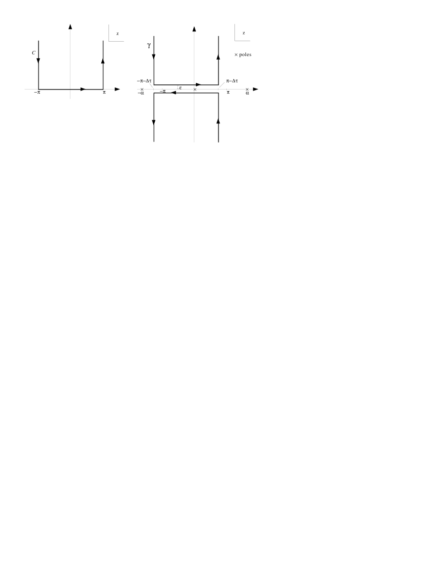
Figure 1.1: Contours $C$ and $\gamma$.

Using this representation we have

$$K_{t}^{\alpha}(x,x^{\prime}|A) = \frac{1}{4\pi\alpha t}e^{-\frac{r^{2}+{r^{\prime}}^{2}}{4t}}\int_{C}dz\,e^{\frac{rr^{\prime}}{2t}\cos z}\sum_{n=-\infty}^{\infty}e^{i\nu_{n}z+i\nu_{n}\Delta\tau},$$

The series is divergent and so it must be regularized: we can use an $\epsilon$-prescription multiplying by $e^{-\epsilon|n|}$:

$$\sum_{n}e^{i\nu|n|z+i\nu n\Delta\tau} \Rightarrow \sum_{n}e^{i\nu|n|z+i\nu n\Delta\tau-\epsilon|n|}$$

$$=1+\sum_{n=1}^{\infty}\left[e^{i(\nu z+\nu\Delta\tau+i\epsilon}\right]^{n}+\sum_{n=1}^{\infty}\left[e^{i(\nu z-\nu\Delta\tau+i\epsilon}\right]^{n}$$

$$=\frac{i}{2}{\mbox{ctg}\,}\left[\frac{1}{2}(\nu(z+\Delta\tau)+i\epsilon)\right]+\frac{i}{2}{\mbox{ctg}\,}\left[\frac{1}{2}(\nu(z-\Delta\tau)+i\epsilon)\right].$$

Then we have

$$K_{t}^{\alpha}(x,x^{\prime}|A) = \frac{i}{8\pi\alpha t}e^{-\frac{r^{2}+{r^{\prime}}^{2}}{4t}}\int_{C}dz\,e^{\frac{rr^{\prime}}{2t}\cos z}\times$$

$$\times\left\{{\mbox{ctg}\,}\left[\frac{1}{2}(\nu(z+\Delta\tau)+i\epsilon)\right]+{\mbox{ctg}\,}\left[\frac{1}{2}(\nu(z-\Delta\tau)+i\epsilon)\right]\right\}.$$

Now we can split the integral in two parts: in the first we change variable to $w=-(z+\Delta\tau+i\epsilon/\nu)$, while in the second $w=z-\Delta\tau+i\epsilon/\nu$. The final result is [45, 41] ($\epsilon/\nu\rightarrow\epsilon$)

$$K_{t}^{\alpha}(x,x^{\prime}|A) = \frac{i}{8\pi\alpha t}\int_{\gamma}dw\,e^{-\frac{r^{2}+{r^{\prime}}^{2}-2rr^{\prime}\cos(w+\Delta\tau)}{4t}}{\mbox{ctg}\,}\frac{\pi w}{\alpha}.$$ (1.23)

Since the flat-space ($\nu=1$) heat kernel is just

$$K_{t}^{\alpha}(x,x^{\prime}|A)=\frac{1}{4\pi t}e^{\frac{(x-x^{\prime})^{2}}{4t}},\hskip 28.45274ptx=(r\cos\tau,r\sin\tau),$$

we can also write the heat kernel on the cone as

$$K_{t}^{\alpha}(x,x^{\prime}|A) = \frac{i}{2\alpha}\int_{\gamma}dw\,{\mbox{ctg}\,}\left(\frac{\pi w}{\alpha}\right)\,K_{t}^{2\pi}(x(w),x^{\prime}|A),$$ (1.24)

where $x(w)=\left(r\cos(\tau+w),r\sin(\tau+w)\right)$.

It is also possible to deform the integration contour $\gamma$ in various ways. For example [41], we can separate the contour into the sum of vertical lines plus the closed Cauchy contour around the poles of ${\mbox{ctg}\,}(\pi w/\alpha)$:

$$K_{t}^{\alpha}(x,x^{\prime}|A) = \frac{1}{4\pi t}{\sum_{n}}^{\prime}e^{-\frac{r^{2}+{r^{\prime}}^{2}-2rr^{\prime}\cos(n\alpha+\Delta\tau)}{4t}}$$

$$+\frac{1}{8\pi\alpha t}\int_{-\infty}^{\infty}dy\,e^{-\frac{r^{2}+{r^{\prime}}^{2}+2rr^{\prime}{\mbox{\tiny ch}\,}y}{4t}}\times$$

$$\times\left\{{\mbox{ctg}\,}\left[\frac{\pi}{\alpha}(iy-\pi-\Delta\tau)\right]+{\mbox{ctg}\,}\left[\frac{\pi}{\alpha}(iy+\pi-\Delta\tau)\right]\right\}.$$

The primed sum is over the $n$ such that $-\pi<n\alpha+\Delta\tau<\pi$. In the coincidence limit $x^{\prime}\rightarrow x$ the above expression can be written as

$$K_{t}^{\alpha}(x,x^{\prime}|A) = \frac{1}{4\pi t}{\sum_{n}}^{\prime}e^{-\frac{r^{2}}{t}\sin^{2}\frac{n\alpha}{2}}$$

$$+\frac{1}{8\pi\alpha t}\int_{-\infty}^{\infty}dy\,e^{-\frac{r^{2}}{t}{\mbox{ch}\,}^{2}\frac{y}{2}}\left\{{\mbox{ctg}\,}\left[\frac{\pi}{\alpha}(iy-\pi)\right]+{\mbox{ctg}\,}\left[\frac{\pi}{\alpha}(iy+\pi)\right]\right\}.$$

Some comments on the behavior of this kernel can be found in [41].

Another useful representation of the heat kernel (1.24) can be obtained for $\Delta\tau<\pi$ by modifying the contour $\gamma$ into a contour $\Gamma$ which consists of two branches, one going from $-\pi-\Delta\tau+i\infty$ to $-\pi-\Delta\tau-i\infty$ and intersecting the real axis very close to the origin, and the other one from $\pi-\Delta\tau+i\infty$ to $\pi-\Delta\tau-i\infty$ in the same way. Then we have [31, 34, 71]

$$K_{t}^{\alpha}(x,x^{\prime}|A) = \frac{1}{4\pi t}e^{-\frac{(x-x^{\prime})^{2}}{4t}}+\frac{i}{8\pi\alpha t}\int_{\Gamma}dw\,e^{-\frac{r^{2}+{r^{\prime}}^{2}-2rr^{\prime}\cos(w+\Delta\tau)}{4t}}{\mbox{ctg}\,}\frac{\pi w}{\alpha}$$ (1.27)

$$= K_{t}^{2\pi}(x,x^{\prime}|A)+\frac{i}{2\alpha}\int_{\Gamma}dw\,{\mbox{ctg}\,}\frac{\pi w}{\alpha}\,K_{t}^{\alpha}(x(w),x^{\prime}|A)$$

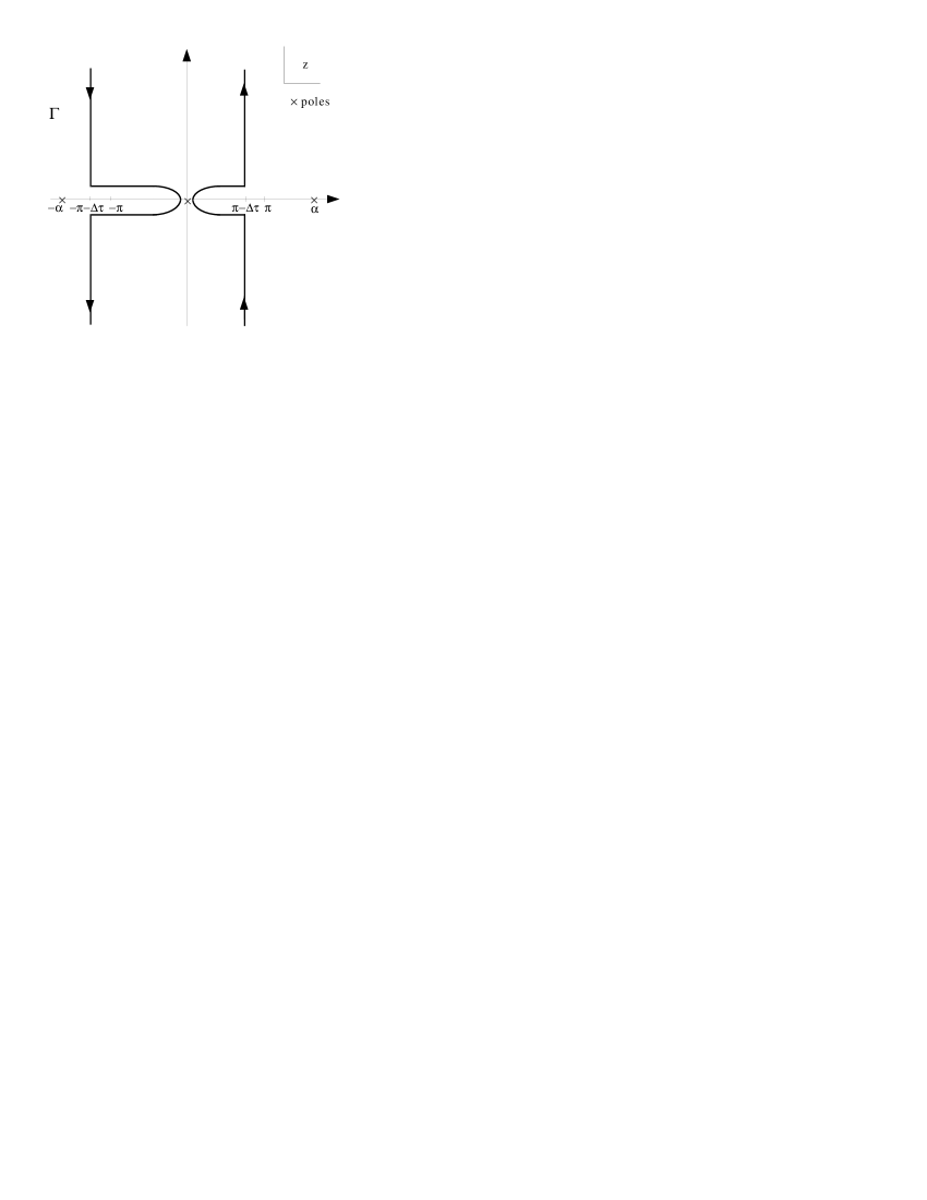
Figure 1.2: Contour $\Gamma$.

The advantage of this representation is that we have isolated the flat-space heat kernel from the conical singularity contribution.

Up to we have considered the local heat kernel. The integrated trace of the kernel can be computed integrating (see Eq. (1.31)) the above representation (1.27) on the cone [107, 33, 47, 34]:

$$\mbox{Tr}\,e^{t\Delta_{\alpha}}=K_{t}^{\alpha}(A)=\frac{V(C_{\alpha})}{4\pi t}+\frac{1}{12}\left(\frac{2\pi}{\alpha}-\frac{\alpha}{2\pi}\right),$$ (1.28)

where $V(C_{\alpha})=\alpha R^{2}/2$ is the (infinite) volume of the cone of radius $R$. The constant term is the conical singularity contribution, first obtained by Kac [107]: the presence of the term $\alpha^{-1}$ implies that it is not a locally computable geometric invariant [33].

1.5.1 Singular heat-kernel expansion

In this section we consider the asymptotic expansion of the heat kernel on the cone considered in the previous section. As a consequence of the singular nature of the curvature at the apex of the cone, we expect that the terms of such an expansion are distributions concentrated at the tip of the cone. Indeed, the expansion has been computed by Cognola et al. [34] and Fursaev [71] (see also [72] and [50]). Because of the distributional nature of the asymptotic expansion we consider it as a functional acting on test functions $f(r,\tau)$ periodic in $\tau$ that we suppose integrable on the cone and such that $rf(r,\tau)$ in infinitely differentiable at $r=0$. Then the asymptotic expansion of the trace reads ($t\rightarrow 0_{+}$)

$$K_{t}^{\alpha}(A) = \mbox{Tr}\,\left(e^{-tA}f\right)=\int d^{2}x\sqrt{g}\,K^{\alpha}_{t}(x,x|A)f(x)$$ (1.29)

$$\simeq \frac{1}{4\pi t}\sum_{n=0}^{\infty}a_{\alpha,n}(f)\,t^{n}.$$

The first coefficient is just the flat space one, and so it reads

$$a_{\alpha,0}(f) = \int d^{2}x\sqrt{g}\,f(x).$$

The other contributions act as Dirac’s delta functions and derivatives at $r=0$ [71]:

$$a_{\alpha,n}(f) = \frac{\Gamma(n)}{(2n-1)!}C_{2n}(\alpha)\int_{0}^{\alpha}d\tau\,\frac{d^{2n-1}}{dr^{2n-1}}rf(r,\tau)|_{r=0},\hskip 14.22636ptn\geq 1,$$ (1.30)

where the coefficients $C_{2n}(\alpha)$ are given by the integrals

$$C_{2n}(\alpha)=\frac{i}{4\alpha}\int_{\Gamma}dw\,\mbox{ctg}\left(\frac{\pi w}{\alpha}\right)\left(\sin^{2}\frac{w}{2}\right)^{-n},$$ (1.31)

and the contour $\Gamma$ is that in figure (1.2). These integrals have been computed by Dowker [47], and the first two are

$$C_{2}(\alpha) = \frac{1}{6}\left[\left(\frac{2\pi}{\alpha}\right)^{2}-1\right]=\frac{\pi}{3\alpha}\left(\frac{2\pi}{\alpha}-\frac{\alpha}{2\pi}\right)=\frac{2\pi}{\alpha}I_{\alpha}(0)$$

$$C_{4}(\alpha) = \frac{1}{15}C_{2}(\alpha)\left[\left(\frac{2\pi}{\alpha}\right)^{2}+11\right]=\frac{2\pi}{\alpha}I_{\alpha}(-1),$$ (1.32)

where we have also reported the relation with the function $I_{\alpha}(z)$ that will be defined in the next section. It is also possible to write a local form for the above expansion [34]:

$$K_{t}^{\alpha}(x,x|A) = \frac{1}{4\pi t}\left[1+\alpha\sum_{k=0}^{\infty}\frac{C_{2k+2}(\alpha)}{2^{k}k!}{\Delta_{\alpha}}^{k}\hat{\delta}(r)\,t^{k+1}\right],$$

where $\hat{\delta}(r)=\delta(r)/r$.

From the above equations we see that the heat-kernel coefficients act like delta functions and derivatives of delta functions at $r=0$, and so they do not depend on the value of $f$ at regular points of the cone: they would never appear if the integration over $r$ is stopped short before $r=0$, no matter how close. This problem, however, affects only the asymptotic expansion, not the integral representations of the local heat kernel we have seen in the previous section.

Another aspect to be remarked of the above expansion is that the half-integer powers of $t$ are absent [34, 72]: this means that, as far as the asymptotic expansion of the heat kernel is concerned, the cone $C_{\alpha}$ does not behave as a two-dimensional manifold with a boundary at $r=0$.

Let us now consider a function which is $1$ in a domain of radius $R$, and zero outside, $f(r,\tau)=\Theta(R-r)$, then the asymptotic series is truncated and one gets the expression exact up to terms that vanish exponentially as $t\rightarrow 0_{+}$ [71]

$$K_{t}^{\alpha}(A)_{R} = \frac{1}{4\pi t}\left(\frac{\alpha R^{2}}{2}+\alpha C_{2}(\alpha)\,t\right)+\mbox{E.S.}$$

$$= \frac{V(C_{\alpha})}{4\pi t}+\frac{1}{12}\left(\frac{2\pi}{\alpha}-\frac{\alpha}{2\pi}\right)+\mbox{E.S.}$$

which is just the expression (1.28) obtained integrating the integral representation of the heat kernel [107, 33], and so we conclude that the exponentially small terms are actually zero.

1.6 $\zeta$ function of the scalar Laplacian on the cone

In the previous section we have studied the heat kernel of the scalar Laplacian on the simple cone $C_{\alpha}$, and we have seen that there are various integral representation of the local heat kernel. In this section we turn our attention to the local $\zeta$ function that, as we have seen in section (1.3), is related to the local heat kernel by a Mellin transform. Nevertheless, we will follow a completely different way to compute the $\zeta$ function, and the final result, instead of an integral representation, will be a meromorphic function. This part is based on the paper [152] by Zerbini et al.. In the final part of this section we will compare the global heat kernel and $\zeta$ function, introducing a new procedure to define the global $\zeta$ function which solves the apparent discrepancy of the two methods.

In the case of the $\zeta$ function on the cone the bibliographic references are much more limited than for the heat kernel. The general theory was developed by Cheeger [33] for manifolds and operators more general than those of interest for us. Other relevant papers in the mathematical literature are those of Brüning and Seeley [22, 23]. Finally, the method of Cheeger was introduced and developed in the physical context by Zerbini et al.[152].

We start by reviewing the Cheeger-Zerbini method for computing the $\zeta$ function on a simple cone $C_{\alpha}\times\mbox{R}^{D-2}$, with metric $ds^{2}=r^{2}d\tau^{2}+dr^{2}+\sum_{i=1}^{D-2}dx_{i}^{2}$, ${\bf x}$ being the transverse flat coordinates. This method will be extensively used in the following Chapters, where, in particular, it will be also extended to the case of a massive scalar field, the Maxwell field and the graviton field.

As for the heat kernel, the starting point is a complete set of normalized eigenfunctions of the Friedrichs extension of minus the Laplace-Beltrami operator $A=-\Delta-\Delta_{\alpha}-\Delta_{D-2}=-(\partial_{r}^{2}+\frac{1}{r}\partial_{r}+\partial_{\tau}^{2}+\sum_{i=1}^{D-2}\partial_{x_{i}}^{2})$. These eigenfunctions read

$$\phi_{n\lambda{\bf k}}(x) = \frac{1}{(2\pi)^{\frac{D-2}{2}}\sqrt{\alpha}}e^{i{\bf k}\cdot{\bf x}-i\frac{2\pi n}{\alpha}\tau}J_{\nu_{n}}(\lambda r),$$

$$A\phi_{n\lambda{\bf k}}(x) = (\lambda^{2}+{\bf k}^{2})\phi_{n\lambda{\bf k}}(x)$$

$$(\phi_{n^{\prime}\lambda^{\prime}{\bf k}^{\prime}}(x),\phi_{n\lambda{\bf k}}(x)) = \int d^{D}x\sqrt{g}\,\phi_{n^{\prime}\lambda^{\prime}{\bf k}^{\prime}}^{\ast}(x)\phi_{n\lambda{\bf k}}(x)$$ (1.33)

$$= \delta_{nn^{\prime}}\delta({\bf k}-{\bf k^{\prime}})\frac{\delta(\lambda-\lambda^{\prime})}{\lambda}.$$

By means of these eigenfunctions we can write the spectral representation of the local $\zeta$ function:

$$\zeta_{\alpha}(s;x|A) = \frac{2}{(4\pi)^{\frac{D-2}{2}}\alpha\Gamma\left(\frac{D-2}{2}\right)}\int_{0}^{\infty}dk\,k^{D-3}\sum_{n=-\infty}^{\infty}\int_{0}^{\infty}\frac{d\lambda\,\lambda}{(\lambda^{2}+k^{2})^{s}}J_{\nu_{n}}^{2}(\lambda r)$$

$$= \frac{\Gamma\left(s-\frac{D-2}{2}\right)}{(4\pi)^{\frac{D-2}{2}}\alpha\Gamma(s)}\sum_{n=-\infty}^{\infty}\int_{0}^{\infty}d\lambda\,\lambda^{D-1-2s}J_{\nu_{n}}^{2}(\lambda r),$$

where we have used $\int d\Omega_{N-1}=2\pi^{N/2}/\Gamma(N/2)$. Now we would have to perform the integration over $\lambda$ and the sum over $n$, but just here we find the main obstacle in the definition of the $\zeta$ function. In fact, for $\frac{D}{2}-\frac{1}{2}<\mbox{Re}\,s<\frac{D}{2}+\nu_{n}$ the integration converges (see [83], formula 6.574.2) and we formally get

$$\zeta_{\alpha}(s;x|A) = \frac{r^{2s-D}\Gamma\left(s-\frac{D-1}{2}\right)}{2\sqrt{\pi}(4\pi)^{\frac{D-2}{2}}\alpha\Gamma(s)}\sum_{n=-\infty}^{\infty}\frac{\Gamma\left(\nu_{n}-s+\frac{D-2}{2}+1\right)}{\Gamma\left(\nu_{n}+s-\frac{D-2}{2}\right)}.$$

However, as it is shown in the appendix of [152], the series converges only for $\mbox{Re}\,s>\frac{D}{2}$, and so the region of convergence does not overlap with that of the integral over $\lambda$.

The solution of this convergence problem has been suggested by Cheeger [33], and it simply consists in a separate treatment of the lower and higher eigenvalues, namely $\nu_{0}=0$ (or $\nu_{n}$, $n<n_{0}$) and $\nu_{n}$, $n\geq 1$ (or $\nu_{n}$, $n\geq n_{0}$). So, one treats separately the terms corresponding to $\nu_{0}$ and $\nu_{n}$, $n\geq 1$, and only after the analytic continuation is performed the two contributions are summed to give the local $\zeta$ function. Of course, such definition of $\zeta$ function has all the requested properties and coincides with the usual definition when the manifold is smooth.

So, following the procedure outlined above, we isolate the term with $n=0$ and define, for $\frac{D}{2}-\frac{1}{2}<\mbox{Re}\,s<\frac{D}{2}$

$$\zeta_{<}(s;x|A) = \frac{r^{2s-D}\Gamma\left(s-\frac{D-1}{2}\right)}{\sqrt{\pi}(4\pi)^{\frac{D-2}{2}}\alpha\Gamma(s)}\frac{\Gamma\left(-s+\frac{D-2}{2}+1\right)}{2\Gamma\left(s-\frac{D-2}{2}\right)}$$

$$= -\frac{r^{2s-D}\Gamma\left(s-\frac{D-1}{2}\right)}{\sqrt{\pi}(4\pi)^{\frac{D-2}{2}}\alpha\Gamma(s)}G_{2\pi}\left(s-{\scriptsize\frac{D-2}{2}}\right).$$

Then we consider all the other terms, performing the integration over $\lambda$ and the summation over $n$. In order to have a common strip of convergence we have to restrict to $\frac{D}{2}<\mbox{Re}\,s<\frac{D}{2}+\nu_{1}$. The result reads

$$\zeta_{>}(s;x|A) = \frac{r^{2s-D}\Gamma\left(s-\frac{D-1}{2}\right)}{\sqrt{\pi}(4\pi)^{\frac{D-2}{2}}\alpha\Gamma(s)}G_{\alpha}\left(s-{\scriptsize\frac{D-2}{2}}\right).$$

where we have set

$$G_{\alpha}(s) = \sum_{n=1}^{\infty}\frac{\Gamma(\nu_{n}-s+1)}{\Gamma(\nu_{n}+s)},$$

$$G_{2\pi} = -\frac{\Gamma(1-s)}{2\Gamma(s)}.$$

The series $G_{\alpha}(s)$ is studied in the appendix of [152], where it is shown that it is convergent for $\mbox{Re}\,s>1$ and that it has an analytic continuation in the whole complex plane showing only a simple pole in $s=1$.

Since both $\zeta_{<}$ and $\zeta_{>}$ can be analytically continued in the whole complex $s$ plane, we can define the local $\zeta$ function as

$$\zeta_{\alpha}(s;x|A) = \zeta_{<}(s;x|A)+\zeta_{>}(s;x|A)$$ (1.34)

$$= \frac{r^{2s-D}}{(4\pi)^{\frac{D-2}{2}}\alpha\Gamma(s)}I_{\alpha}\left(s-{\scriptsize\frac{D-2}{2}}\right),$$

where

$$I_{\alpha}(s) \equiv \frac{\Gamma(s-1/2)}{\sqrt{\pi}}\left[G_{\alpha}(s)-G_{2\pi}(s)\right].$$ (1.35)

The properties of the function $I_{\alpha}(s)$ are studied in the appendix of [152] (see also [99]): it has only a simple pole in $s=1$ with residue ($\nu=2\pi/\alpha$)

$$\mbox{Res }I_{\alpha}(s)|_{s=1} = \frac{1}{2}\left(\nu^{-1}-1\right),$$

and near the pole [99]

$$I_{\alpha}(s) = \frac{1}{2(s-1)}(\nu^{-1}-1)+\frac{1}{2}(\nu^{-1}-1)(\gamma-2\ln 2)-\frac{\ln\nu}{\nu}+{\cal O}(s-1).$$

Finally, important values of $I_{\alpha}(s)$ are

$$I_{\alpha}(0) = \frac{1}{6\nu}(\nu^{2}-1)$$

$$I_{\alpha}(-1) = \frac{1}{90\nu}(\nu^{2}-1)(\nu^{2}+11),$$

and, by definition, $I_{2\pi}(s)=0$.

1.6.1 Global $\zeta$ function

Let us now consider the global $\zeta$ function. From the mathematical point of view, only the local $\zeta$ function has a precise meaning, because of the non-integrable singularity in $r=0$. As a consequence, for defining global quantities one has to introduce some kind of regularization by means of a smearing function $f(r)$ with compact support not containing the origin. Of course, it is also necessary to control the volume divergences in the transverse dimensions, which integrated give an infinite volume ${\cal A}_{\Sigma}$. Thus, we define the smeared trace as [152]

$$\zeta_{\alpha}(s|A)_{f} = \alpha{\cal A}_{\Sigma}\int_{0}^{\infty}dr\,r\,\zeta_{\alpha}(s;x|A)f(r)$$ (1.36)

$$= \frac{{\cal A}_{\Sigma}}{(4\pi)^{\frac{D-2}{2}}\Gamma(s)}I_{\alpha}\left(s-{\scriptsize\frac{D-2}{2}}\right){\hat{f}}(2s-D+2),$$

where

$${\hat{f}}(s) = \int_{0}^{\infty}dr\,r^{s-1}\,f(r)$$

is the Mellin transform of $f(r)$. The function ${\hat{f}}(s)$ is analytic since the integral in (1.36) exists for all $s$ by definition. So, we see that the only possible singularity of $\zeta_{\alpha}(s|A)_{f}$ is that coming from $I_{\alpha}(s)$ in $s=1$. The simplest choice of smearing function is $f(r)=\Theta(R-r)\Theta(r-\epsilon)$, which is convergent to $1$ as $R\rightarrow\infty$ and $\epsilon\rightarrow 0$. Thus, we have ${\hat{f}}(s)=(R^{s}-\epsilon^{s})/s$ and [152]

$$\zeta_{\alpha}(s|A)_{f} = \frac{{\cal A}_{\Sigma}}{(4\pi)^{\frac{D-2}{2}}\Gamma(s)}I_{\alpha}\left(s-{\scriptsize\frac{D-2}{2}}\right)\frac{R^{2s-D+2}-\epsilon^{2s-D+2}}{2s-D+2}.$$

There is also an alternative procedure to define the integrated $\zeta$ function on the cone, and it is the following. Let us consider $\zeta_{<}(s;x|A)$ and $\zeta_{>}(s;x|A)$ before the analytic continuation procedure. They are defined for $\frac{D}{2}-\frac{1}{2}<\mbox{Re}\,s<\frac{D}{2}$ and $\frac{D}{2}<\mbox{Re}\,s<\frac{D}{2}+\nu_{1}$ respectively. In both these strips of the complex $s$ plane, $r^{2s-D}$ does not give rise to non-integrable singularities in $r=0$, and so we can integrate them over $r$ separately, provided we regulate the harmless volume divergence at $r\rightarrow\infty$, for instance by means of $\Theta(R-r)$. After the integration we can analytically continue each piece and sum. The final result is

$$\zeta_{\alpha}(s|A)_{R} = \frac{{\cal A}_{\Sigma}}{(4\pi)^{\frac{D-2}{2}}\Gamma(s)}I_{\alpha}\left(s-{\scriptsize\frac{D-2}{2}}\right)\frac{R^{2s-D+2}}{2s-D+2}.$$ (1.37)

An important property of this $\zeta$ function is that we have an extra pole in $s=\frac{D-2}{2}$, besides the one in $s=\frac{D}{2}$ coming from $I_{\alpha}(s)$.

Let us now study the relation of these two definitions of the integrated $\zeta$ function with the asymptotic heat kernel expansion. Notice that we will not try to compare the local $\zeta$ function with the local asymptotic expansion of the heat kernel, since the distributional nature of the local Seeley-DeWitt coefficients cannot be seen from the local $\zeta$ function.

For the sake of simplicity we consider the case $D=4$. The asymptotic expansion reads

$$K_{t}^{\alpha}(A)\simeq\frac{1}{(4\pi t)^{2}}\sum_{n=0}^{\infty}A_{n}\,t^{n},$$

where on $C_{\alpha}\times\mbox{R}^{2}$ (see Eq. (1.28))

$$A_{0} = {\cal{A}}_{\Sigma}V(C_{\alpha}),$$

$$A_{1} = \frac{\pi{\cal{A}}_{\Sigma}}{3}\left(\frac{2\pi}{\alpha}-\frac{\alpha}{2\pi}\right)=2\pi{\cal{A}}_{\Sigma}I_{\alpha}(0),$$

and $A_{n}=0$, $n>1$. From Eq. (1.10) we know that the meromorphic structure of the $\zeta$ function is related to the Seeley-DeWitt coefficients by

$$\zeta(s|A)=\frac{1}{16\pi^{2}\Gamma(s)}\frac{A_{0}}{s-2}+\frac{1}{16\pi^{2}\Gamma(s)}\frac{A_{1}}{s-1}+h(s),$$

where $h(s)$ is an analytic function. Therefore, we expect for $\zeta(s|A)$ two simple poles in $s=2$ and $s=1$, which is not the case in $\zeta(s|A)_{f}$, that has only a simple pole in $s=2$. Instead, the two poles correctly appear in the proposed regularization $\zeta(s|A)_{R}$. In fact, the pole structure of $\zeta(s|A)_{R}$ is

$$\zeta(s|A)_{R} = \frac{{\cal{A}}_{\Sigma}\alpha R^{2}}{32\pi^{2}(s-2)}\left(1-\frac{2\pi}{\alpha}\right)+\frac{{\cal{A}}_{\Sigma}I_{\alpha}(0)}{8\pi(s-1)}+g(s)$$ (1.38)

$$= \frac{A_{0}}{16\pi^{2}(s-2)}\left(1-\frac{2\pi}{\alpha}\right)+\frac{A_{1}}{16\pi^{2}(s-1)}+g(s),$$

where $g(s)$ is an analytic function. The discrepancy in the residue of the pole in $s=2$ is easily explained. It is shown in [152] that the Mellin transform of the local heat kernel does not correspond to $\zeta_{\alpha}(s;x|A)$, but rather to $\zeta_{\alpha}(s;x|A)-\frac{2\pi}{\alpha}\zeta_{2\pi}(s;x|A)$, where the Cheeger-Zerbini analytic procedure gives $\zeta_{2\pi}(s;x|A)=0$. Hence the term

$$-\frac{A_{0}}{16\pi^{2}(s-2)}\frac{2\pi}{\alpha}=-\frac{{\cal{A}}_{\Sigma}\pi R^{2}}{16\pi^{2}(s-2)}$$

is just the flat space contribution in the asymptotic expansion.Therefore, we see that by means of this alternative procedure for taking the trace of the local $\zeta$ function we get a complete agreement with the integrated heat kernel.

One could wonder which one is the correct procedure, but this question has not a simple answer. The problem can be summarized as follows. If one is simply interested in the computation of the integrated heat kernel from the local one, then there is no doubt that the correct result is given in Eq. (1.28). However, if one wants to compute one-loop quantities from the local heat kernel, then the question is more subtle and involves a conflict between the regularization of the divergent integral over the manifold in $r=0$ and the regularization of the ultraviolet divergences, namely the analytic continuation procedure in the $\zeta$ function or some other procedure employing the heat kernel, such as the dimensional one. We will see that, if the ultraviolet divergences are regularized in the local quantities, then the ultraviolet regularized local quantities diverge in $r=0$ and some cut-off in the integration over the manifold is necessary. This procedure corresponds to the one which leads to Eq. (1.36). On the other hand, if we integrate the local quantities before the ultraviolet regularization, then no cut-off in $r=0$ is needed. This procedure clearly corresponds to the second one, which leads to Eq. (1.37).

It is important to stress that the problem is to choose the order in which the two regularization have to be performed, and probably this problem cannot be solved by mathematical reasoning, for which both procedures are equally correct. We postpone this topic to Chapter 4, where we will use physical requirements to argue that the correct procedure is the first one, Eq. (1.36).

Chapter 2 $\zeta$-function regularization and one-loop renormalization of field fluctuations in curved space-time

Introduction

This Chapter, based on the paper [102], is devoted to improve the $\zeta$-function approach to regularize and renormalize the averaged square field $\langle\phi^{2}(x)\rangle$ in a general curved background.

The quantity $\langle\phi^{2}(x)\rangle$ has been studied by several authors [15] because its knowledge is an important step to proceed within the point-splitting renormalization of the stress tensor and also due to its importance in cosmological theories. The knowledge of the value of $\langle\phi^{2}(x)\rangle$ is also necessary to get the renormalized Hamiltonian from the renormalized stress tensor in non minimally coupled theories, and this is important dealing with thermodynamical considerations [61, 117]. Furthermore, the quantity $\langle\phi^{2}(x)\rangle$ gives a measure of the vacuum distortion due, for instance, to a boundary, and so it is of great interest in the study of Casimir’s effects (see, e.g., [14, 1]).

Let us consider a generic Euclidean field theory in a curved background ${\cal M}$ corresponding to the Euclidean action

$$S_{A}[\phi]=-\frac{1}{2}\int_{\cal M}d^{4}x\sqrt{g}\>\phi A\phi,$$ (2.1)

where Euclidean motion operator $A$ is supposed self-adjoint and positive-definite. The local $\zeta$ function related to the operator $A$, $\zeta(s,x|A)$, can be defined as the analytic continuation of the series [91, 56, 53]

$$\zeta(s,x|A)={\sum_{n}}^{\prime}\lambda_{n}^{-s}\phi_{n}^{*}(x)\phi_{n}(x).$$ (2.2)

where $\{\phi_{n}(x)\}$ is a complete set of normalized eigenvectors of $A$ with eigenvalues $\lambda_{n}$, and ^′ means that, in the sum, the null eigenvectors are omitted. In (2.2), the right hand side is supposed to be analytically continued in the whole $s$-complex plane. Indeed, it is well-known that the $\zeta$ function is a meromorphic function with, at most, simple poles situated at $s=1$ and $s=2$ in case of a four dimensional compact (Euclidean) spacetime without boundaries. Since we assume a compact spacetime, we work with a discrete spectrum, but all considerations can be trivially extended to operators with continuous spectrum. The importance of the $\zeta$ function is that its derivative evaluated at $s=0$ defines a regularization of the one-loop effective action:

$$S_{\mbox{\scriptsize eff}}[\phi,g]=\left.-\frac{1}{2}\frac{d}{ds}\right|_{s=0}\zeta(s,x|A/\mu^{2}),$$ (2.3)

where $\mu$ is an arbitrary parameter with the dimensions of a mass necessary from dimensional considerations. Recently, the method has been extended in order to define a similar $\zeta$-function regularization directly for the renormalized stress tensor [117].

The usual approach to compute the field fluctuations by means of the $\zeta$-function technique leads to the following naïve definition for the one-loop averaged square field

$$\langle\phi^{2}(x)\rangle:=\zeta(s,x|A)|_{s=1},$$ (2.4)

This definition follows directly from (2.2) taking account of the spectral decomposition of the two-point function. Anyhow, barring exceptional situations (e.g. see [116]), this definition is not available because the presence of a pole at $s=1$ in the analytically continued $\zeta$ function, and so a further infinite subtraction procedure seems to be necessary. Conversely, in the cases of the effective action and stress tensor regularization, the $\zeta$-function approach leads naturally to the complete cancellation of divergences maintaining the finite $\mu$-parameterized counterterms physically necessary [117]. We shall see shortly that, also in the case of $\langle\phi^{2}(x)\rangle$, it is possible to improve the $\zeta$-function approach to get the same features: cancellation of all divergences and maintenance of the finite $\mu$-parameterized counterterms. This fact will allow us to get the one-loop renormalized field fluctuations of a scalar field in Einstein’s closed universe for the massive/non-conformally-coupled case. As we shall say, this result can be achieved in several other ultrastatic spacetime with constant spatial curvature. Finally, our definition will allow us to give a formula for the trace of the stress tensor of a generally non-conformally invariant field in which all quantities are regularized by means of the $\zeta$-function approach.

2.1 The general approach

Let us define the $\zeta$ function of $\langle\phi^{2}(x)\rangle$. To get a definition of the $\zeta$ function regularization of the field fluctuations we shall follow an heuristic way already considered in other papers for different aims [35, 117, 121]. Let us consider the one-loop effective action in the presence of an external source $J(x)$

$$S_{\scriptsize\mbox{eff}}[g_{ab},J]=\ln\int{\cal D}\phi\>e^{S_{A}[J]}=\ln\int{\cal D}\phi\>e^{S_{A}-\frac{1}{2}\int d^{4}x\sqrt{g}\>J\phi^{2}}.$$ (2.5)

We have

$$\langle\phi^{2}(x)\rangle=-\left.\frac{2}{\sqrt{g(x)}}\>\frac{\delta S_{\scriptsize\mbox{eff}}}{\delta J(x)}\right|_{J(x)\equiv 0}.$$ (2.6)

From the $\zeta$-function regularization, and supposing to be possible to interchange the order of the $J$ functional derivative and the $s$ derivative we can formally write, in a purely heuristic view

$$\langle\phi^{2}(x)\rangle=\left.\frac{d\>\>}{ds}\right|_{s=0}\frac{1}{\sqrt{g(x)}}\frac{\delta\zeta(s|A/\mu^{2})}{\delta J(x)}|_{J(x)\equiv 0}.$$ (2.7)

Still heuristically, we can also write

$$\frac{\delta\zeta(s|A/\mu^{2})}{\delta J(x)}={\sum_{n}}^{\prime}\frac{\delta(\lambda_{n}/\mu^{2})^{-s}}{\delta J(x)}=-s{\sum_{n}}^{\prime}\frac{\delta(\lambda_{n}/\mu^{2})}{\delta J(x)}\left(\frac{\lambda_{n}}{\mu^{2}}\right)^{-(s+1)},$$ (2.8)

where one can use the relation (obtained as in Appendix of [117])

$$\left.\frac{\delta\lambda_{n}}{\delta J(x)}\right|_{J\equiv 0}=-\phi_{n}^{*}(x)\phi_{n}(x)\sqrt{g(x)}.$$ (2.9)

Supposing to analytically continue the right hand side of (2.8) as far as is possible in the complex $s$ plane, through (2.7), (2.8), (2.9) and (2.2) we are led very naturally to the following definition of the $\zeta$-function regularization of the field fluctuations, which we shall assume without further justifications

$$\langle\phi^{2}(x)\rangle:=\left.\frac{d\>\>}{ds}\right|_{s=0}\>\frac{s}{\mu^{2}}\>\zeta(s+1,x|A/\mu^{2}).$$ (2.10)

The identity above can be written down also as

$$\langle\phi^{2}(x)\rangle:=\left.\frac{d\>\>}{ds}\right|_{s=0}Z(s,x|A/\mu^{2})\>,$$

where we have defined

$$Z(s,x|A/\mu^{2}):=\frac{s}{\mu^{2}}\>\zeta(s+1,x|A/\mu^{2})$$

the local $\zeta$ function of the field fluctuations. This function has essentially the same meromorphic structure as the function $\zeta(s+1,x|A/\mu^{2})$ except for the fact that the simple pole at $s=0$ in $\zeta(s+1,x|A/\mu^{2})$, whenever it exists, is now canceled out by the factor $s$. Moreover, when $\zeta(s+1,x|A/\mu^{2})$ is regular at $s=0$ the definition in (2.10) coincides with the naive one, Eq. (2.4). The scale $\mu$ represents the usual ambiguity due to a remaining finite renormalization (already found concerning the effective action and the stress tensor[15, 148, 117]) and it remains into the final result whenever another fixed scale is already present in the theory. Two final remarks are in order. First we notice that Eq. (2.10) can be also written as

$$\langle\phi^{2}(x)\rangle=\left.\frac{d\>\>}{ds}\right|_{s=0}\>s\>\zeta(s+1,x|A)+\ s\zeta(s+1,x|A)|_{s=0}\ln\mu^{2}.$$ (2.11)

Secondly, from the well-known (see, e.g., [15, 14, 17]) asymptotic expansion of the local heat kernel on manifolds without boundary

$$K_{t}(x|A)\simeq\frac{1}{(4\pi)^{D/2}}\sum_{j=0}^{\infty}a_{j}(x|A)t^{j-D/2},$$

it is easy to show that the $\zeta$ function has a pole in $s=1$ if and only if the dimension $D$ is even and the coefficient $a_{\frac{D}{2}-1}(x|A)$ is non-vanishing. Therefore, in odd dimensions we can use the definition (2.4) of the fluctuations, while in even dimensions we can also rewrite (2.11) as

$$\langle\phi^{2}(x)\rangle:=\lim_{s\rightarrow 1}\left[\zeta(s,x|A)-\frac{a_{\frac{D}{2}-1}(x|A)}{(4\pi)^{D/2}\Gamma(s)(s-1)}\right]+\frac{\gamma+\ln\mu^{2}}{(4\pi)^{D/2}}a_{\frac{D}{2}-1}(x|A),$$

where $\gamma$ is Euler’s constant. From this expression, it is clear that the disappearance of $\mu$ from the final result is equivalent to the possibility of using the naive definition (2.4). In four dimensions we have that $a_{1}=\frac{1}{6}(1-6\xi)R(x)-m^{2}$, and so (2.4) is available either for the massless case with vanishing scalar curvature or for the massless conformal coupling case, $\xi=1/6$.

We finish this section giving a general formula for the trace of the stress tensor of a non-conformal scalar field. It is well known [15] that in the case of a non-conformally invariant field such trace is the sum of two contributions, an anomalous one and a non-anomalous one. Classically, the trace can be computed from the variation of the classical action under a conformal transformation $g_{ab}\rightarrow\lambda(x)g_{ab}$, $\phi(x)\rightarrow\lambda^{(2-D)/4}(x)\phi(x)$:

$$g^{ab}T_{ab}(x) = -\left.\frac{2\lambda(x)}{\sqrt{g}}\frac{\delta S[m,\xi]}{\delta\lambda(x)}\right|_{\lambda=1}.$$

Now we write the action as $S[m,\xi]=S[m=0,\xi=m]-\frac{1}{2}\int\phi[m^{2}+\xi R]\phi\,\sqrt{g}d^{D}x$: by making the variation on both sides, using also the conformal invariance of $S[m=0,\xi=\xi_{D}]$, we arrive to the following expression:

$$-\frac{2}{\sqrt{g}}g^{ab}\frac{\delta S[m,\xi]}{\delta g^{ab}} = -\frac{D-2}{2}\phi^{\ast}A\phi+\left[\frac{1}{2\xi_{D}}(\xi_{D}-\xi)\Delta-m^{2}\right]\phi^{\ast}\phi.$$

Then, following the method introduced in [117], we evaluate this expression on the modes $\phi_{n}$ of the operator $A$, multiply by $\lambda_{n}^{-s-1}$, sum over the non-null modes and analytically continue the obtained expressions. The result reads

$$g^{ab}\zeta_{ab}(s+1,x|A) = -\frac{D-2}{2}\zeta(s,x|A)$$ (2.12)

$$+\left[\frac{1}{2\xi_{D}}(\xi_{D}-\xi)\Delta-m^{2}\right]\zeta(s+1,x|A),$$

where the tensorial $\zeta$ function, $\zeta_{ab}(s,x|A)$, is that defined in [117]. Finally, we multiply Eq. (2.12) by $s\mu^{-2}$ and take the derivative at $s=0$: remembering the definitions of [117] and the definition (2.10), we get the final expression for the trace of the stress tensor for a non-conformally invariant scalar field:

$$g^{ab}\langle T_{ab}(x)\rangle = \zeta(0,x|A)+\left[\frac{1}{2\xi_{D}}(\xi_{D}-\xi)\Delta-m^{2}\right]\langle\phi^{2}(x)\rangle$$ (2.13)

$$= \frac{a_{D/2}(x)}{(4\pi)^{D/2}}+\left[\frac{1}{2\xi_{D}}(\xi_{D}-\xi)\Delta-m^{2}\right]\langle\phi^{2}(x)\rangle.$$

We clearly identify the contribution coming from the conformal anomaly and the non-anomalous contribution which depends on the quantum state chosen. The above expression is formally equivalent to a corresponding formula containing also derivative terms given in [15] which has to be further regularized. Such a formal equivalence can be proven by employing the formal motion equation for the field operator $\hat{\phi}$ in the formula in [15]. Conversely, we remark that in our expression all quantities are already consistently regularized by means of the same $\zeta$-function procedure taking also account of the scale $\mu$ which appears in both sides of Eq. (2.13).

2.2 Some applications and comments

Let us consider now some simple applications in order to check on the correctness of our procedure. First we consider two cases in which the simplest formula (2.4) may be used giving correct results. Let us consider a scalar massless field in Minkowski spacetime contained in a large box at the temperature $\beta$. The local $\zeta$ function is easily obtained (see [91]) and reads

$$\zeta(s,x|A/\mu^{2})=\frac{\sqrt{\pi}\mu^{4}}{(2\pi)^{3}}\left(\frac{2\pi}{\beta\mu}\right)^{4-2s}\frac{\Gamma(s-3/2)}{\Gamma(s)}\zeta_{R}(2s-3),$$

where $\zeta_{R}(s)$ is the usual Riemann zeta function. Notice that no pole appears at $s=1$, hence we could also use the naive definition (2.4) instead of (2.10). In both cases the result is

$$\langle\phi^{2}(x)\rangle_{\beta}=\frac{1}{12\beta^{2}}.$$

This result is the same which follows from other approaches, for instance subtracting the Minkowski massless zero-temperature two-point function from the thermal one and performing the limit of coincidence of the arguments.

Consider now the Casimir effect due to two infinite parallel planes on which the field is constrained to vanish, namely we consider a massless scalar field in the Euclidean manifold $[0,L]\times R^{3}$. In this case the local $\zeta$ function can be computed by taking the Mellin transform of the corresponding heat kernel, which is given, e.g., in [1]. A straightforward computation yields ($0<x<L/2$)

$$\zeta(s,x|A/\mu^{2}) = \frac{L^{2s-4}\Gamma(2-s)}{16\pi^{2}\Gamma(s)}\times$$

$$\times\left[2\zeta_{R}(4-2s)+\left(\frac{x}{L}\right)^{2s-4}-2\zeta_{R}(4-2s,x/L)\right].$$

We see that the $\zeta$ function is regular at $s=1$ and so the fluctuations can be computed in the naive way:

$$\langle\phi^{2}(x)\rangle_{\beta} = \frac{1}{48L^{2}}-\frac{1}{8\pi^{2}L^{2}}\left[\zeta_{R}(2,x/L)-\frac{L^{2}}{2x^{2}}\right]$$

$$= \frac{1}{48L^{2}}\left[1-3\mbox{csc}^{2}\frac{\pi x}{L}\right]$$

$$\sim -\frac{1}{16\pi^{2}x^{2}}+{\cal O}(x^{0}).$$

This result is in agreement with the known one (see, e.g., [69]), but $\zeta$-function approach saves much labour.

Now, let us consider other cases where one is forced to use (2.10). The simplest case is represented by a scalar field in Minkowski space time at zero temperature. As it is well known [1], for a massless field the corresponding $\zeta$ function can be considered as vanishing, as follows also from the limit $\beta\rightarrow\infty$ in first example considered, and so we pass directly to the massive case. The local $\zeta$ function in four dimensions reads

$$\zeta(s,x|A/\mu^{2})=\frac{m^{4}(\mu/m)^{2s}}{16\pi^{2}(s-1)(s-2)},$$

which has a simple pole at $s=1$. Using (2.10) we immediately obtain the correct Coleman-Weinberg-like [32] result

$$\langle\phi^{2}(x)\rangle=\frac{m^{2}}{16\pi^{2}}\left[2\ln\frac{m}{\mu}-1\right].$$ (2.14)

As a simple application on a curved background we may start considering the field fluctuations of a massless conformally coupled scalar field on the closed static Einstein universe with spatial section metric $a^{2}[dX^{2}+\sin^{2}X(d\theta^{2}+\sin^{2}\theta d\varphi^{2})]$. The spatial section of this manifold is the $3$-sphere $S^{3}$ with curvature $R=6/a^{2}$, $a$ being the radius of the sphere. This case has been considered in several papers (see [15]) and, more recently, in [117] employing the $\zeta$-function approach for a (generally thermal) massless conformally coupled scalar field. In this simplest case

$$\zeta(s,x|A)=\frac{1}{4\pi^{1/2}V}\frac{\Gamma(s-3/2)}{\Gamma(s)}(2s-3)a^{2s-1}\zeta_{R}(2s-3),$$ (2.15)

where $V=V(a)=2\pi^{2}a^{3}$ is the spatial volume of the universe. This function has no pole at $s=1$ but takes a pole at $s=2$. Through (2.4), we have the well-known result which can be achieved by other approaches with a similar amount of work [15]

$$\langle\phi^{2}(x)\rangle=\zeta(1,x|A/\mu^{2})=-\frac{1}{48\pi^{2}a^{2}}.$$ (2.16)

Unlike other approaches and in a very direct and elegant way, employing our improved procedure (2.10) and some technical results found out in [29] we are able to compute the vacuum fluctuations also in the case of a non-conformal coupling and/or in the presence of a massive field, when the $\zeta$ function does take a pole at $s=1$. The Euclidean operator reads

$$A=-\Delta+\xi R+m^{2}=A_{0}/a^{2},$$ (2.17)

As any finite value of the mass can be interpreted in terms of a redefinition of $\xi$ ($R$ is constant) $\xi\rightarrow\xi^{\prime}=\xi+m^{2}/R$, we shall explicitly consider the case $m=0$ only. From $\zeta(s,x|A)=a^{2(s-2)}\zeta(s,x|A_{0})$ we have

$$a^{2}\langle\phi^{2}(x)\rangle=\left.\frac{d\>\>}{ds}\right|_{s=0}\>s\zeta(s+1,x|A_{0})+s\zeta(s+1,x|A_{0})|_{s=0}\ln(\mu^{2}a^{2}),$$ (2.18)

where $\langle\phi^{2}(x)\rangle$ is referred to $A$ and not to $A_{0}$. Notice that the argument of the logarithm is adimensional: the natural scale already present in the theory is $a$. Using particular cases of the equations (11.78), (11.85) and (12.19) in [29] and (2.15) for the the case $a=1$, we find

$$s\zeta(s+1,x|A_{0}) = \frac{1}{2V_{0}\pi^{1/2}}\frac{\Gamma(s+3/2)}{\Gamma(s)}\left[(1-6\xi)\zeta_{R}(2s+1)-\delta_{\xi 0}\right]$$

$$+\frac{1}{2V_{0}\pi^{1/2}}\sum_{n=0,n\neq 1}^{+\infty}\frac{\Gamma(s+n+1/2)}{n!\Gamma(s)}\left[(1-6\xi)^{n}\zeta_{R}(2s+2n-1)-\delta_{\xi 0}\right].$$

This equation holds for $0\leq 6\xi<2$ (i.e., replacing $\xi$ which appears in the equation above with $\xi^{\prime}$ defined previously, $0\leq 6\xi+a^{2}m^{2}<2$), so it includes both the minimal coupling $\xi=0$ and the conformal coupling $\xi=1/6$. The series converges everywhere in $s$ complex plane away from the poles of the function $\zeta$ and $\Gamma$ in the various numerators (see [29] for a general discussion). Notice that the pole at $s=1$ of $\zeta(s,x|A_{0})$ in the case of a non-conformal coupling arises from a corresponding pole in the term $n=1$ of the series above which has been made explicit in the first term in the right hand side of (LABEL:lunga). This pole at $s=1$ is nothing but the pole at $s=2$ which is present in the conformal coupled $\zeta$ function. Finally, taking also account that (2.4) can be used in the (massless) conformal case, Eq. (2.18) leads us to the relationship between $\langle\phi^{2}(x)\rangle_{\xi}$ and $\langle\phi^{2}(x)\rangle_{\xi=1/6}$

$$\langle\phi^{2}(x)\rangle_{\xi} = \langle\phi^{2}(x)\rangle_{\xi=1/6}+\frac{1-6\xi}{4V}(1+\gamma-\ln 2)$$ (2.20)

$$+ \frac{1}{2V\pi^{1/2}}\sum_{n=2}^{+\infty}\frac{\Gamma(n+1/2)}{n!}\left[(1-6\xi)^{n}\zeta_{R}(2n-1)-\delta_{\xi 0}\right]$$

$$- \frac{3\delta_{\xi 0}}{4V}+\ln(a^{2}\mu^{2})\frac{1-6\xi}{8V}.$$

The series in (2.20) converges for $0\leq 6\xi<2$ at least, as one can check employing Stirling’s estimate of the $\Gamma$ function and $\zeta(s)=1+2^{-s}+{\cal O}(3^{-s})$ for large positive values of $s$.

To generalize the relation (2.20), let us consider a massless field (the mass can be restored by a trivial redefinition of $\xi$, as $R$ is a constant) propagating in an ultrastatic manifold with the topology of $R\times{\cal M}$, where the second factor is a $3$-dimensional compact rank one symmetric space (the procedure can be generalized considering higher dimensions). The metric reads $ds^{2}=-dt^{2}+a^{2}ds^{2}_{{\cal M}}$. Employing results found out in [29], we get

$$s\zeta_{\xi}(s+1,x|A_{0}) = \frac{(\rho^{2}-\xi R_{0})\Gamma(s+2)}{\Gamma(s)}\zeta_{\xi=1/6}(s+2,x|A_{0})$$ (2.21)

$$-\frac{\delta_{\xi 0}\Gamma(s+3/2)}{2V_{0}\pi^{1/2}\rho^{2s+1}}$$

$$+\sum_{n=0,n\neq 1}^{+\infty}\left[\frac{(\rho^{2}-\xi R_{0})^{n}\Gamma(s+n+1)}{n!\Gamma(s)}\zeta_{\xi=1/6}(s+n+1,x|A_{0})\right.$$

$$\left.-\frac{\delta_{\xi 0}\Gamma(s+n+1/2)}{2V_{0}n!\pi^{1/2}\rho^{2s+1}}\right].$$

We have set $\rho^{2}:=R_{0}/6$ ($\rho>0$) and $R_{0},A_{0},V_{0}$ are referred to the metric with $a=1$. The series converges for $0\leq\xi R_{0}<2\rho^{2}$ away from the explicit poles (see [29]). In spite of the notations, the various local $\zeta$ functions which appear above do not depend on $x$ because of the symmetry of the space and so do the corresponding fluctuations of the field. Also in this case, the pole at $s=1$ of the general $\zeta$ function is related with that at $s=2$ in the conformally coupled $\zeta$ function. Once again, (2.10) and (2.4) for the conformal case, lead us to

$$\langle\phi^{2}(x)\rangle_{\xi} = \langle\phi^{2}(x)\rangle_{\xi=1/6}-\frac{3}{4V}\frac{\delta_{\xi 0}}{\rho}+\ln(\mu^{2}a^{2})\left(\rho^{2}/a^{2}-\xi R\right)P$$ (2.22)

$$+\sum_{n=2}^{+\infty}\left[\frac{(\rho^{2}/a^{2}-\xi R)^{n}\Gamma(n+1)}{n!}\zeta_{\xi=1/6}(n+1,x|A)-\frac{\delta_{\xi 0}\Gamma(n+1/2)}{2Vn!\pi^{1/2}\rho}\right]$$

$$+\left(\rho^{2}/a^{2}-\xi R\right)P+\left(\rho^{2}/a^{2}-\xi R\right)\frac{d\>\>}{ds}|_{s=0}s\zeta_{\xi=1/6}(s+2,x|A),$$

where we have set $P=\lim_{s\rightarrow 0}s\zeta_{\xi=1/6}(s+2,x|A)=a_{0}(x|A)/(4\pi)^{2}$ and, for $n>2$, $\zeta_{\xi=1/6}(n,x|A)$ is the arguments coincidence limit of the Green function of $A^{n}_{\xi=1/6}$. Up to the knowledge of the authors, this is the first time that equations as (2.20) and (2.22) appear in the literature and there is no analogous relation obtained employing approaches different from the $\zeta$ function one.

Chapter 3 Massive scalar field

Introduction

In this Chapter, based on the paper [99], we discuss the extension of the local $\zeta$ function on the cone to the case of massive fields. As we have partially seen in Chapter 1, many techniques have been developed to compute relevant quantities in presence of conical singularities (see, among the others, [45, 33, 47, 41, 5, 80, 108, 34, 71, 75, 152]). With few exceptions [34, 71, 111, 129, 86, 87, 114], most authors considered massless fields only. Indeed, the introduction of the mass complicates the problem considerably, so that it becomes very difficult to obtain manageable forms for the physical quantities. In this regard, it has to be noted that using the integrated heat-kernel approach [34, 71] it seems that all the problems vanish: in fact, for a scalar field of mass $m$ the integrated heat-kernel is simply related to the massless one as

$$K_{t}^{m}=e^{-tm^{2}}K_{t}^{m=0},$$ (3.1)

and, at least for a simple cone $R^{D-2}\times C_{\alpha}$, the integrated massless heat-kernel is well known [33, 34, 71] (see Eq. (1.28):

$$K_{t}^{m=0}=\frac{\Sigma_{D-2}}{(4\pi t)^{2}}\left[\frac{V(C_{\alpha})}{4\pi t}+\frac{1}{12}\left(\frac{2\pi}{\alpha}-\frac{\alpha}{2\pi}\right)\right],$$

where $2\pi-\alpha$ is the deficit angle of the cone, $V(C_{\alpha})$ is the volume of the cone and $\Sigma_{D-2}$ is the volume of the transverse dimensions. In contrast to the massless case, the Mellin transform of Eq. (3.1) exists in the massive case, and so it is easy to compute the massive global $\zeta$ function and from it quantities like the effective action, which have a simple closed form. However, it is well known [152] that this procedure does not yield the correct dependence on the deficit angle of the cone in the massless limit and, moreover, these global quantities are finite, apart for the volume divergences, while the local quantities show a non-integrable singularity near the tip of the cone. Therefore, it is at least dubious that this simple result for the massive case is correct. Besides, in order to compute important quantities such as the vacuum fluctuations of the field and the stress tensor, local rather than global quantities are needed. The problems related to the local and integrated approaches on the cone will be discussed in Chapter 4.

The aim of this Chapter is to give a more manageable tool for computing local quantities for a massive scalar field around a cosmic string or at finite temperature in the Rindler wedge. To avoid any confusion, we will focus on the cosmic string case, but all the results we will obtain are easily translated to the case of fields at finite temperature in the Rindler space or near the horizon of a Schwarzschild black hole. We will accomplish this result by computing the local $\zeta$ function, which will be given as an expansion in powers of $mr$, where $r$ is the distance form the string core. Therefore, the obtained expressions are useful near the string, where $mr\ll 1$. However, since the local quantities diverge at the string core, this is just the interesting region if, for instance, one wants to consider the back-reaction of the energy-momentum tensor on the background metric [97, 85]. The expression we obtain is simple enough to allow us to compute the renormalized vacuum expectation value $\langle\phi^{2}(x)\rangle$ and the the energy-momentum tensor, potentially up to arbitrary order in $(mr)^{2}$. Notice that the most common tool used to compute local quantities is the Green’s function, which in the massive case is given in a complicated integral form [111, 129, 87, 34] or as a sum of generalized hypergeometric functions [114].

As we said above, we are mainly concerned in the comic-string background. We remind that the space-time around an infinitely long, static and straight cosmic string [146] has the topology ${\cal M}^{4}=R^{2}\times C_{\alpha}$, where $C_{\alpha}$ is the simple two-dimensional cone with deficit angle $2\pi-\alpha$, and the metric is

$$ds^{2} = -dt^{2}+dz^{2}+dr^{2}+r^{2}d\theta^{2},$$ (3.2)

$$\hskip 56.9055ptr\in(0,+\infty),\,\,\theta\in[0,\alpha],\,\,t,z\in(-\infty,+\infty).$$

The polar angle deficit $2\pi-\alpha$ is related to the mass per unit length of the string $\mu$ by $2\pi-\alpha=8\pi G\mu$. Throughout this chapter we shall assume positive deficit angle, so that $\nu\equiv 2\pi/\alpha>1$. For GUT strings $\nu-1\sim 10^{-6}$ [146]. In the rest of the chapter we adopt an Euclidean approach and so we perform a Wick rotation $\tau=it$: the form of the metric is the same as above with the replacement $-dt^{2}\rightarrow+d\tau^{2}$. Moreover, for technical reasons we will also consider the obvious generalization to the $D$-dimensional case, with topology $R^{D-2}\times C_{\alpha}$.

We have assumed zero thickness for the string: this is clearly an idealization, since an actual cosmic string should have a small but finite radius, of the order of the Compton wavelength of the Higgs boson involved in the phase transition which gives rise to the cosmic string [146]. The internal structure of the string has non-negligible effects even at large distances, as it has been shown by Allen, Kay, and Ottewill [4]. However, in the same work it has been shown that for a minimally coupled scalar this dependence on the internal structure is absent, and one can safely use the idealized string. In order to avoid the complications discussed in [4], which are related to the non-uniqueness of the self-adjoint extension of the Laplace-Beltrami operator in the idealized conical space-time, we shall consider the minimally coupled case only. Actually, in Sec. IV we will compute the stress tensor and, for sake of completeness, we will consider arbitrary coupling. Therefore, we have to remember that for $\xi\neq 0$ others effects could be present in a realistic cosmic string.

The rest of this chapter is organized as follows. In section 3.1 we compute the $\zeta$ function of a massive scalar field in the cosmic-string background. Then we use this result to compute, in the region $mr\ll 1$, the vacuum fluctuations of the field in section 3.2 and the expectation value of the stress tensor in section 3.3. In section 3.4 we employ the stress tensor to compute the backreaction on the metric of the idealized cosmic string, in the context of of the semiclassical approach to quantum gravity. Section 3.5 contains the conclusions.

3.1 Computation of the $\zeta$ function

We consider a quasi-free real scalar field in the background given by the (Wick-rotated) metric (3.2). The action of the theory is the given by

$$S[\phi] = \frac{1}{2}\int d^{D}x\sqrt{g}\,\phi A\phi,$$

where $A$ is known as the small fluctuations operator and in our case reads

$$A = -\Delta_{D}+m^{2}+\xi R.$$ (3.3)

Here $\xi$ is a parameter which fixes the coupling of the field to the gravity by means of the scalar curvature $R$. We shall consider the minimally coupled case, $\xi=0$. Then, by means standard passages one sees that the generating functional of the theory can be expressed in terms of the functional determinant of the small fluctuations operator, which can be conveniently defined by means of the $\zeta$ function regularization [91] (see Chapter 1):

$$\ln Z_{\alpha} = -\frac{1}{2}\ln\det\mu^{-2}A=\frac{1}{2}\zeta^{\prime}(0|A\mu^{-2})$$

where $\zeta(s|A)$ is the global $\zeta$ function related to the operator $A$, the prime indicates the derivative with respect to $s$ and $\mu$ is an arbitrary parameter with the dimensions of a mass needed for dimensional reasons and not to be confused with the mass per unit length of the string. The global $\zeta$ function can be formally written as the integral over the manifold of a local $\zeta$ function $\zeta(s|A)(x)$:

$$\zeta(s|A) = \int_{{\cal M}^{D}_{\alpha}}\zeta(s|A)(x)\sqrt{g}d^{D}x.$$

Actually, when the manifold is non-compact only the local $\zeta$ function has a precise mathematical meaning, since the integration requires the introduction of cutoffs or smearing functions to avoid divergences.

In the massless case, the $\zeta$ function on the cone has been explicitly computed in [152] (see section 1.6). In order to compute it in the massive case, the starting point is the well known relation between the local $\zeta$ function and the heat kernel given by the Mellin transform:

$$\zeta^{m}(s;x)=\frac{1}{\Gamma(s)}\int_{0}^{\infty}dt\,t^{s-1}K_{t}(x).$$

The heat kernel of the massive field is related to the massless one by means of the following obvious decomposition:

$$K_{t}^{m}(x)=e^{-tm^{2}}K_{t}^{m=0}(x).$$

Now we take into account the following property of the Mellin transform of the product of two functions [26]

$$\int_{0}^{\infty}t^{s-1}f(t)g(t)dt=\frac{1}{2\pi i}\int_{\sigma-i\infty}^{\sigma-i\infty}F(z)G(s-z)dz,$$

where $F$ and $G$ are the Mellin transforms of $f$ and $g$ respectively and $\sigma$ is a real number in the common strip of convergence of the two Mellin transforms. In this way we can write the massive $\zeta$ function of in terms of the massless one:

$$\zeta^{m}(s;x)=\frac{1}{2\pi i\Gamma(s)}\int_{\sigma-i\infty}^{\sigma-i\infty}\Gamma(z)\zeta^{m=0}(z;x)m^{2z-2s}\Gamma(s-z)dz,$$ (3.4)

where we have used the Mellin transform

$$\int_{0}^{\infty}t^{s-1}e^{-tm^{2}}dt=m^{-2s}\Gamma(s),$$

which converges for $\mbox{Re}s>0$.

Since we are interested in the $\zeta$ function of a massive scalar field in the (Euclidean) space $R^{D-2}\times C_{\alpha}$, we consider the corresponding massless $\zeta$ function. It has been shown in [33] and [152] that it is the sum of two parts which converge in separate strips of the complex $s$-plane and which are summed only after their analytic continuation:

$$\zeta^{m=0}(z;x)=\zeta_{<}(s;x)+\zeta_{>}(s;x),$$

where

$$\zeta_{<}(s;x) = \frac{r^{2s-D}}{\alpha(4\pi)^{\frac{D-2}{2}}\Gamma(s)}\frac{\Gamma(s-\frac{D-1}{2})\Gamma(\frac{D}{2}-s)}{2\sqrt{\pi}\Gamma(s-\frac{D-2}{2})},$$

$$\hskip 113.81102pt\mbox{for }\frac{D-1}{2}<\mbox{Re }s<\frac{D}{2},$$

$$\zeta_{>}(s;x) = \frac{r^{2s-D}}{\alpha(4\pi)^{\frac{D-2}{2}}\Gamma(s)}\frac{\Gamma(s-\frac{D-1}{2})}{\sqrt{\pi}}G_{\alpha}(s-{\scriptstyle\frac{D-2}{2}}),$$

$$\hskip 113.81102pt\mbox{for }\frac{D}{2}<\mbox{Re }s<\frac{D}{2}+\nu,$$

and the function $G_{\alpha}(s)$ is defined as

$$G_{\alpha}(s)=\sum_{n=1}^{\infty}\frac{\Gamma(\nu_{n}-s+1)}{\Gamma(\nu_{n}+s)},\hskip 28.45274pt\nu_{n}=\frac{2\pi}{\alpha}|n|,\hskip 14.22636pt\nu\equiv\nu_{1}$$

and can be analytically continued in the whole complex plane showing simple poles in $s=1$, with residue $\alpha/4\pi$, and $s=\nu_{n}+k+1$, $k=0,1,2,\dots,$ (if $\alpha\neq 2\pi$) with obvious residue. Since $\zeta_{<}$ and $\zeta_{>}$ do not have a common strip of convergence, we must split Eq. (3.4) in two parts: setting $\mbox{Re}s>D/2$ we have

$$\zeta_{>}^{m}(s;x) = \frac{1}{2\pi i\Gamma(s)}\frac{r^{-D}m^{-2s}}{(4\pi)^{\frac{D-2}{2}}\sqrt{\pi}\alpha}\times$$

$$\times\int_{\scriptsize\frac{D}{2}<{\mbox{\scriptsize Re}\,}z<{\mbox{\scriptsize Re}\,}s}dz\,\Gamma(z-{\scriptstyle\frac{D-1}{2}})G_{\alpha}(z-{\scriptstyle\frac{D-2}{2}})\Gamma(s-z)(mr)^{2z}$$

$$=\frac{r^{2s-D}}{(4\pi)^{\frac{D-2}{2}}\sqrt{\pi}\alpha\Gamma(s)}\left\{\sum_{n=0}^{\infty}\frac{(-1)^{n}}{n!}(mr)^{2n}\Gamma(s+n-{\scriptstyle\frac{D-1}{2}})G_{\alpha}(s+n-{\scriptstyle\frac{D-2}{2}})\right.$$

$$+\left.(mr)^{D-2s}\sum_{n=1}^{\infty}\sum_{k=0}^{\infty}\frac{(-1)^{k}}{k!}\frac{\Gamma(\nu_{n}+k+1/2)}{\Gamma(2\nu_{n}+k+1)}\Gamma(s-\nu_{n}-k-{\scriptstyle\frac{D}{2}})(mr)^{2\nu_{n}+2k}\right\},$$

where we have performed the integral shifting the integration path to the right and picking up the residues of the poles of the integrand. The same procedure can be applied to $\zeta_{<}^{m}(s;x)$, but in this case we have to consider the poles in $z=s+n$ and $z=2+n$:

$$\zeta_{<}^{m}(s;x) = \frac{1}{2\pi i\Gamma(s)}\frac{r^{-D}m^{-2s}}{(4\pi)^{\frac{D-2}{2}}\sqrt{\pi}\alpha}\times$$

$$\times\int_{\scriptsize\frac{D-1}{2}<{\mbox{\scriptsize Re}\,}z<{\mbox{\scriptsize Re}\,}\frac{D}{2}}dz\,\frac{\Gamma(z-\frac{D-1}{2})\Gamma(\frac{D}{2}-z)}{2\Gamma(z+1-D/2)}\Gamma(s-z)(mr)^{2z}$$

$$=\frac{r^{2s-D}}{(4\pi)^{\frac{D-2}{2}}\sqrt{\pi}\alpha\Gamma(s)}\left\{\sum_{n=0}^{\infty}\frac{(-1)^{n}}{n!}(mr)^{2n}\frac{\Gamma(s+n-\frac{D-1}{2})\Gamma(\frac{D}{2}-s-n)}{2\Gamma(s+n+1-D/2)}\right.$$

$$\left.+(mr)^{D-2s}\sum_{n=0}^{\infty}\frac{(-1)^{n}}{n!}(mr)^{2n}\frac{\Gamma(n+1/2)\Gamma(s-n-D/2)}{2\Gamma(n+1)}\right\}.$$

Now we analytically continue each term and sum to get the final expression of the local $\zeta$ function of a massive scalar field:

$$\zeta^{m}(s;x) = \frac{r^{2s-D}\mu^{2s}}{(4\pi)^{\frac{D-2}{2}}\alpha\Gamma(s)}\left\{\sum_{n=0}^{\infty}\frac{(-1)^{n}}{n!}(mr)^{2n}I_{\alpha}(s+n-{\scriptstyle\frac{D-2}{2}})\right.$$

$$+\frac{(mr)^{D-2s}}{\sqrt{\pi}}\sum_{n=0}^{\infty}\frac{(-1)^{n}}{n!}(mr)^{2n}\frac{\Gamma(n+1/2)\Gamma(s-n-D/2)}{2\Gamma(n+1)}$$

$$\left.+\frac{(mr)^{D-2s}}{\sqrt{\pi}}\sum_{n=1}^{\infty}\sum_{k=0}^{\infty}\frac{(-1)^{k}}{k!}\frac{\Gamma(\nu_{n}+k+1/2)}{\Gamma(2\nu_{n}+k+1)}\Gamma(s-\nu_{n}-k-{\scriptstyle\frac{D}{2}})(mr)^{2\nu_{n}+2k}\right\},$$

where the function $I_{\alpha}(s)$ is that defined in Eq. (1.35). In expression (LABEL:zetafun) we have also reintroduced the arbitrary mass $\mu$ using the formal relation $\zeta(s|A\mu^{-2})=\mu^{2s}\zeta(s|A)$, and which has been omitted in the derivation for simplicity. It must be noted that the above $\zeta$ function can be obtained in a more direct way, albeit much longer, performing the integrations in the Mellin transform of the spectral representation of the massive heat kernel, and then rearranging the sums and the Euler gamma functions in the generalized hypergeometric functions obtained by the integrations. We prefer the used method since it can be more easily applied to the computation of others quantities, as we will see in the next sections. Moreover, this method based of the Mellin transform could be useful in other cases to treat the massive case when the massless $\zeta$ function is known.

Although expression (LABEL:zetafun) looks awful, it is very simple when $mr\ll 1$: considering the physically interesting case $D=4$ and terms up to $(mr)^{4}$

$$\zeta^{m}(s;x) = \frac{r^{2s-4}\mu^{2s}}{4\pi\alpha\Gamma(s)}\left[I_{\alpha}(s-1)-(mr)^{2}I_{\alpha}(s)\right.$$

$$\left.+\frac{1}{2}(mr)^{4}I_{\alpha}(s+1)+{\cal O}\left((mr)^{6}\right)\right]$$

$$+\frac{m^{4}(m/\mu)^{-2s}}{8\pi\alpha\Gamma(s)}\left[\Gamma(s-2)-\frac{(mr)^{2}}{2}\Gamma(s-3)\right.$$

$$\left.+2(mr)^{2\nu}\frac{\Gamma(\nu+1/2)\Gamma(s-\nu-2)}{\sqrt{\pi}\Gamma(2\nu+1)}+{\cal O}\left((mr)^{4}\right)\right].$$

In the first term of the first row we recognize the massless $\zeta$ function on $R^{2}\times C_{\alpha}$ [152], while the first term in the second row becomes the $\zeta$ function of a massive scalar field in the Minkowski space-time when $\alpha=2\pi$ [1]. The others terms are clearly corrections due to the presence of the conical singularity. When the singularity is absent, namely when $\alpha=2\pi$, the first row vanishes, since $I_{2\pi}(s)=0$, while in the second and third rows only the first term survives, since the others cancel two by two.

At the same order in $mr$, the effective lagrangian density is given by

$${\cal L}(x) = -\frac{1}{2}\frac{d}{ds}\zeta^{m}(s;x)|_{s=0}$$

$$= -\frac{1}{8\pi\alpha r^{4}}\left\{I_{\alpha}(-1)-(mr)^{2}I_{\alpha}(0)\right.$$

$$-\frac{(mr)^{4}}{2}\left[\frac{\nu-1}{\nu}\left(\gamma+\ln\frac{{r\mu}}{2}\right)+\frac{\ln\nu}{\nu}+\ln\frac{m}{\mu}-\frac{3}{4}\right]$$

$$-\frac{(mr)^{6}}{24}\left[2G_{\alpha}(2)+2\gamma+2\ln\frac{mr}{2}-\frac{11}{6}\right]$$

$$\left.+2(mr)^{2\nu+4}\frac{\Gamma(\nu+\frac{1}{2})\Gamma(-\nu-2)}{\sqrt{\pi}\Gamma(2\nu+1)}\right\}.$$

where $G_{\alpha}(n)$, $n\geq 2$, are readily computed being in the region of convergence of the series defining $G_{\alpha}$. For example

$$G_{\alpha}(2) = -\frac{1}{2\nu}\left[2\gamma+\psi\left(\nu^{-1}\right)+\psi\left(-\nu^{-1}\right)\right],$$

$$G_{\alpha}(3) = -\frac{1}{6\nu}\left[3\gamma-\psi\left(\nu^{-1}\right)-3\psi\left(-\nu^{-1}\right)+\psi\left(-2\nu^{-1}\right)\right],$$

where $\psi(x)=\Gamma^{\prime}(x)/\Gamma(x)$. In the limit $\alpha\rightarrow 2\pi$ the above effective lagrangian reduces to the usual Coleman-Weinberg potential. It is important to note that the computation of higher orders in the above expansion in powers of $(mr)^{2}$ does not involve particular complications.

3.2 Vacuum fluctuations

Now we use the above $\zeta$ function to compute the (renormalized) value of the vacuum fluctuations of the field. We start considering the naïve definition (2.4) [1]:

$$\langle\phi^{2}(x)\rangle = \lim_{s\rightarrow 1}\zeta(s;x).$$

Since even in the Minkowski space the vacuum expectation value diverges, we renormalize the vacuum expectation value on the cone subtracting the Minkowski value: in this way we have a remarkable cancellation of the poles, yielding a finite result:

$$\langle\phi^{2}(x)\rangle_{\alpha}-\langle\phi^{2}(x)\rangle_{2\pi} =$$ (3.6)

$$\frac{1}{4\pi\alpha r^{2}}\left\{I_{\alpha}(0)+\frac{(mr)^{2}}{\nu}\left[(\nu-1)\left(\ln\frac{mr}{2}+\gamma-\frac{1}{2}\right)+\ln\nu\right]\right.$$

$$+\frac{(mr)^{4}}{8}\left[2G_{\alpha}(2)+2\gamma-1+2\ln\frac{mr}{2}\right]$$

$$\left.+(mr)^{2\nu+2}\frac{\Gamma(\nu+1/2)\Gamma(-\nu-1)}{\sqrt{\pi}\Gamma(2\nu+1)}+{\cal O}\left((mr)^{6}\right)\right\}.$$

The computation of higher corrections is straightforward. One can verify that Eq. (3.6) correctly vanishes in the limit $\alpha\rightarrow 2\pi$, and that up to order $(mr)^{2}$ it is identical to the result obtained by Moreira Jnr. [114]. In particular, we notice the additional logarithmic divergences of the vacuum fluctuations at the conical singularity due to the massive corrections.

Let us now compute the same vacuum fluctuations employing the improved definition (2.10): in this case no explicit subtraction is needed and, considering only terms up to order $(mr)^{2}$, the result is

$$\langle\phi^{2}(x)\rangle_{\alpha} = \frac{1}{4\pi\alpha r^{2}}\left\{I_{\alpha}(0)+\frac{(mr)^{2}}{\nu}\left[(\nu-1)\left(\gamma+\ln\frac{r\mu}{2}\right)\right.\right.$$ (3.7)

$$\left.\left.+\ln\nu+\frac{\nu}{2}\left(2\ln\frac{m}{\mu}-1\right)\right]\right\}.$$

The above expression is different from the result obtained by subtracting the Minkowski value and in fact reduces to the Minkowski value, Eq. (2.14), rather than vanishing when the conical singularity is removed, namely $\nu\rightarrow 1$. We note that in the massless case both procedures give the same result, since the massless $\zeta$ function is regular at $s=1$. On the other hand, the arbitrariness in the choice of the reference state to be subtracted appears in (3.7) in the form of a dependence on the arbitrary mass parameter $\mu$: changing $\mu$ is equivalent to a change in the subtraction point. Indeed, the difference between two results for the vacuum fluctuations can be written as

$$\frac{(mr)^{2}}{8\pi^{2}r^{2}}\left[\ln\frac{m}{\mu}-\frac{1}{2}\right].$$

So, e.g., if one chooses $\mu=m/\sqrt{e}$ then Eq. (3.7) reproduces exactly Eq. (3.6).

3.3 Energy-momentum tensor

Another important vacuum average is that of the energy-momentum tensor. While in the massless case it is quite easy to be computed, since its form is fixed from symmetry arguments, in the massive case the computation is much more difficult and, to our knowledge, the massive corrections near the string have never been shown explicitly. Only in [129] and [87] the explicit form of the energy-momentum tensor has been given for $mr\gg 1$, where they found the expected exponential damping factor $\exp(-2mr)$.

We use a point-splitting approach, in which the vacuum expectation value of the energy momentum tensor is given by the coincidence limit of a non-local differential operator applied to the regularized and renormalized propagator of the field [15]:

$$\langle T_{\mu\nu}(x)\rangle=i\lim_{x^{\prime}\rightarrow x}D_{\mu\nu}(x,x^{\prime})G_{\cal F}(x,x^{\prime}),$$

where

$$D_{\mu\nu}(x,x^{\prime}) \equiv (1-2\xi)\nabla_{\mu}\nabla_{\nu^{\prime}}+-2\xi\nabla_{\mu}\nabla_{\nu}+(2\xi-\frac{1}{2})g_{\mu\nu}\left[\nabla_{\alpha}\nabla^{\alpha^{\prime}}-m^{2}\right],$$

and the prime indicates that the derivative has to be taken with respect to $x^{\prime}$. Since the propagator can be obtained from the off-diagonal $\zeta$ function [15] as

$$G_{\cal F}(x,x^{\prime})=i\lim_{s\rightarrow 1}\zeta(s;x,x^{\prime}),$$

we can compute the energy momentum tensor from the $\zeta$ function as (see also [91, 35])

$$\langle T_{\mu\nu}(x)\rangle=-\lim_{s\rightarrow 1}\lim_{x^{\prime}\rightarrow x}D_{\mu\nu}(x,x^{\prime})\zeta(s;x,x^{\prime}).$$

The partial derivatives of the off-diagonal $\zeta$ function which appear in the above expression can be computed from the spectral representation in $D$ dimensions (${\bf x}\equiv(\tau,{\vec{z}})$, $k=|{\bf k}|$)

$$\zeta_{D}(s;x,x^{\prime}) = \frac{2(4\pi)^{-\frac{D-2}{2}}}{\alpha\Gamma(\frac{D-2}{2})}\int_{0}^{\infty}dk\,k^{D-3}\sum_{n=-\infty}^{\infty}\int_{0}^{\infty}d\lambda\,\lambda[\lambda^{2}+k^{2}+m^{2}]^{-s}$$

$$\times J_{\nu_{n}}(\lambda r^{\prime})J_{\nu_{n}}(\lambda r)e^{i{\bf k}\cdot({\bf x}-{\bf x}^{\prime})+i\frac{2\pi}{\alpha}n(\theta-\theta^{\prime})},$$

and then taking the coincidence limit. In this way one can easily show that

$$\partial_{\theta}\partial_{\theta^{\prime}}\zeta_{D}(s;x,x^{\prime})|_{x=x^{\prime}} = -\partial_{\theta}^{2}\zeta_{D}(s;x,x^{\prime})|_{x=x^{\prime}}$$

$$\partial_{z_{i}}\partial_{{z_{i}}^{\prime}}\zeta_{D}(s;x,x^{\prime})|_{x=x^{\prime}} = -\partial_{z_{i}}^{2}\zeta_{D}(s;x,x^{\prime})|_{x=x^{\prime}}=2\pi\zeta_{D+2}(s;x)$$

$$\partial_{\tau}\partial_{\tau^{\prime}}\zeta_{D}(s;x,x^{\prime})|_{x=x^{\prime}} = -\partial_{\tau}^{2}\zeta_{D}(s;x,x^{\prime})|_{x=x^{\prime}}=2\pi\zeta_{D+2}(s;x)$$

$$\partial_{r^{\prime}}\zeta_{D}(s;x,x^{\prime})|_{x=x^{\prime}} = \frac{1}{2}\partial_{r}\zeta_{D}(s;x).$$

As far as $\partial_{\theta}^{2}\zeta_{D}(s;x,x^{\prime})|_{x=x^{\prime}}$ is concerned, in the $m=0$ case it is easy to see that we have

$$\partial_{\theta}^{2}\zeta_{D}^{m=0}(s;x,x^{\prime})|_{x=x^{\prime}}=-\frac{r^{2s-D}\Gamma(s-\frac{D-1}{2})}{(4\pi)^{\frac{D-2}{2}}\sqrt{\pi}\alpha\Gamma(s)}H_{\alpha}(s-{\scriptstyle\frac{D-2}{2}}),$$

where the function $H_{\alpha}(s)$ is defined and studied in the Appendix A. The massive case can then be treated using the off-diagonal version of Eq. (3.4) with the partial coincidence limit $r=r^{\prime}$, $z=z^{\prime}$ and $t=t^{\prime}$:

$$\partial_{\theta}^{2}\zeta_{4}(s;\theta,\theta^{\prime})|_{\theta=\theta^{\prime}} = \frac{1}{2\pi i\Gamma(s)}\int\Gamma(z)\partial_{\theta}^{2}\zeta_{4}^{m=0}(z;\theta,\theta^{\prime})|_{\theta=\theta^{\prime}}\Gamma(s-z)m^{2z-2s}dz$$

$$=\frac{-1}{2\pi i\Gamma(s)}\int_{\mbox{\scriptsize Re }z>3}\frac{r^{2z-4}}{4\pi\sqrt{\pi}\alpha}\Gamma(z-3/2)H_{\alpha}(z-1)\Gamma(s-z)m^{2z-2s}dz.$$

$$=-\frac{r^{2s-4}\mu^{2s}}{4\pi\sqrt{\pi}\alpha\Gamma(s)}\left\{\sum_{n=0}^{\infty}\frac{(-1)^{n}}{n!}(mr)^{2n}\Gamma(s+n-3/2)H_{\alpha}(s+n-1)\right.$$

$$\left.+(mr)^{4-2s}\sum_{n=1}^{\infty}\sum_{k=0}^{\infty}\frac{(-1)^{k}}{k!}(mr)^{2\nu_{n}+2k}\nu_{n}^{2}\frac{\Gamma(s-\nu_{n}-k-2)\Gamma(\nu_{n}+k+1/2)}{\Gamma(2\nu_{n}+k+1)}\right\}.$$

where, as usual, we have performed the integration shifting the integration contour to the right and picking up the residues at $z=s+n$ and $z=\nu_{n}+k+2$ to get an expansion in powers of $mr$ similar to Eq. (LABEL:zetafun).

As far as the second derivatives with respect to $r$ and $r^{\prime}$ are concerned, using the following identity, which can be proved using some recursion formulas for the Bessel functions [83],

$$[\partial_{r}J_{\nu}(\lambda r)]^{2}=-\frac{\nu^{2}}{r^{2}}J_{\nu}^{2}(\lambda r)+\frac{1}{2r}\partial_{r}r\partial_{r}J_{\nu}^{2}(\lambda r)+\lambda^{2}J_{\nu}^{2}(\lambda r),$$

one can see that

$$\partial_{r}\partial_{r^{\prime}}\zeta_{D}(s;x,x^{\prime})|_{x=x^{\prime}} = \frac{1}{2r}\partial_{r}r\partial_{r}\zeta_{D}(s;x)+\frac{1}{r^{2}}\partial_{\theta}^{2}\zeta_{D}(s;x,x^{\prime})|_{x=x^{\prime}}$$

$$+\chi_{D}(s;x),$$

$$\partial^{2}_{r^{\prime}}\zeta_{D}(s;x,x^{\prime})|_{x=x^{\prime}} = -\frac{1}{2r}\partial_{r}\zeta_{D}(s;x)-\frac{1}{r^{2}}\partial_{\theta}^{2}\zeta_{D}(s;x,x^{\prime})|_{x=x^{\prime}}$$

$$-\chi_{D}(s;x),$$

where the function $\chi_{D}(s;x)$ is defined in Appendix B. If $D=4$ and $m=0$ we simply have

$$\chi_{D=4}^{m=0}(s;x)=4\pi(s-2)\zeta_{D=6}^{m=0}(s;x),$$ (3.9)

while the massive case is more complicate and is studied in the Appendix B.

Now we have all the pieces needed to compute the massive correction to the energy-momentum tensor. For the actual calculation it is convenient to follow [21] and [3]. We define the renormalized stress tensor as

$$\langle T_{\mu\nu}(x)\rangle_{\alpha}^{R}\equiv\langle T_{\mu\nu}(x)\rangle_{\alpha}-\langle T_{\mu\nu}(x)\rangle_{2\pi}$$

which, considering only the first massive correction, turns out to be

$$\langle T_{\theta\theta}\rangle_{\alpha}^{R} = \frac{1}{4\pi\alpha r^{2}}\left[2H_{\alpha}(0)-(6\xi-1)I_{\alpha}(0)+(mr)^{2}\left(H_{\alpha}(1)+\xi\frac{\nu-1}{\nu}\right)\right],$$

$$\langle T_{rr}\rangle_{\alpha}^{R} = \frac{-1}{4\pi\alpha r^{4}}\left[2H_{\alpha}(0)-I_{\alpha}(-1)-(2\xi-1)I_{\alpha}(0)\right.$$

$$\left.+(mr)^{2}\left(H_{\alpha}(1)+\xi\frac{\nu-1}{\nu}\right)\right],$$

$$\langle T_{tt}\rangle_{\alpha}^{R} = \frac{-1}{8\pi\alpha r^{4}}\left[I_{\alpha}(-1)+2(4\xi-1)I_{\alpha}(0)+(mr)^{2}I_{\alpha}(0)\right],$$

$$\langle T_{zz}\rangle_{\alpha}^{R} = \langle T_{tt}(x)\rangle_{\alpha}^{R},$$

The tensor can be written in the more familiar form

$$\langle{T_{\mu}}^{\nu}(x)\rangle_{\alpha}^{R} = \frac{-1}{1440\pi^{2}r^{4}}\left[\left(\nu^{4}-1\right)\mbox{diag}(1,1,-3,1)\right.$$ (3.10)

$$\left.+10(6\xi-1)\left(\nu^{2}-1\right)\mbox{diag}(2,-1,3,2)\right.$$

$$+15(mr)^{2}(\nu-1)(12\xi-1-\nu)\mbox{diag}(0,1,-1,0)$$

$$\left.+15(mr)^{2}\left(\nu^{2}-1\right)\mbox{diag}(1,0,0,1)\right].$$

In the limit $m\rightarrow 0$ the result is in agreement with that obtained by other authors [47, 67]. The components $\langle T_{rr}(x)\rangle_{\alpha}^{R}$ and $\langle T_{\theta\theta}(x)\rangle_{\alpha}^{R}$ satisfy the equation

$$\frac{d}{dr}(r{T^{r}}_{r}) = {T^{\theta}}_{\theta},$$

which follows from the conservation law $\nabla_{\mu}{T^{\mu}}_{\nu}=0$. Another interesting check of the above result is the comparison with the conformal anomaly formula, Eq. (2.13). For a massive scalar field and general coupling, the trace of the one-loop renormalized stress tensor is given by an anomalous contribution $\zeta(s=0;x)$ and a non-anomalous contribution which depends on the quantum state chosen [15]:

$$\langle{T_{\mu}}^{\mu}(x)\rangle^{R} = \zeta(s=0;x)+\left[\frac{1}{2}(1-6\xi)\Delta-m^{2}\right]\langle\phi^{2}(x)\rangle.$$

Although Eq. (2.13) was derived employing the $\zeta$-function regularization of [117] also for the energy momentum tensor, it can be applied also for our mixed $\zeta$-function and point-splitting method, provided that we employ the expression (3.6) for the fluctuations in order to have a subtraction scheme consistent with that of the stress tensor. It is then easy to check that this relation is satisfied by the quantities computed above, order by order in $(mR)^{2}$.

It is interesting to notice that in the corrections to the stress tensor of order $(mr)^{2}$ are not present the logarithmic divergences which are instead present in the vacuum fluctuations at the same order (see Eq. (3.6)). The logarithmic terms appear in higher order corrections, which can also be computed with the method we have developed. Actually only the logarithms in the term of order $(mr)^{4}$ give rise to divergences, since at higher orders they are multiplied by positive powers of $r$. Indeed, the correction of order $(mr)^{4}$ to $\langle T_{\theta\theta}(x)\rangle_{\alpha}^{R}$ is

$$\frac{1}{4\pi\alpha r^{2}}\left\{-\frac{(mr)^{4}}{8}\left[2\frac{\ln\nu+1}{\nu}+(2\xi-1)A(r)+4\xi-1\right]\right.$$

$$\left.+(mr)^{2+2\nu}\nu[2\xi+(4\xi-1)\nu]\frac{\Gamma(-\nu-1)\Gamma(\nu+1/2)}{\sqrt{\pi}\Gamma(2\nu+1)}\right\},$$

from which one can also compute the correction to $\langle T_{rr}(x)\rangle_{\alpha}^{R}$ by means of the conservation law. The correction to $\langle T_{tt}(x)\rangle_{\alpha}^{R}=\langle T_{zz}(x)\rangle_{\alpha}^{R}$ is

$$-\frac{1}{8\pi\alpha r^{4}}\left\{\frac{(mr)^{4}}{4}\left[2B(r)-(4\xi-1)(A(r)+1)-\frac{1}{\nu}\right]\right.$$

$$\left.+(mr)^{2+2\nu}2(4\xi-1)\nu^{2}\frac{\Gamma(-\nu-1)\Gamma(\nu+1/2)}{\sqrt{\pi}\Gamma(2\nu+1)}\right\}.$$

In the above equations we have set

$$A(r) = 2G_{\alpha}(2)+2\gamma+2\ln\frac{mr}{2}.$$

$$B(r) = \frac{\nu-1}{\nu}\left(\ln\frac{mr}{2}+\gamma-\frac{1}{2}\right)+\frac{\ln\nu}{\nu}.$$

An interesting point to be discussed is the dependence on the parameter $\xi$ which fixes the coupling of the scalar field with the gravity. In the introduction we said that we would consider the minimally coupled case only, $\xi=0$: this because it has been shown in [4] that the idealized conical space is a good model of the space time of a cosmic string only for the minimally coupled case. For nonminimally coupled fields quantities like $\langle\phi^{2}(x)\rangle$ will depend on the details of the metric in the core of the string even very far from the string. However, one could be interested, e.g., in finite-temperature fields in the Rindler space, where the (Euclidean) manifold there is a true conical singularity and not just an idealization of a non-singular metric. In these cases it is interesting to consider also nonminimally coupled fields.

It is clear that in a realistic model of cosmic string all the quantities may depend on the parameter $\xi$. Moreover, during the process of renormalization of the theory the dependence on $\xi$ can appear even in the case $R=0$, and actually, in an interacting theory this parameter becomes a running coupling constant (see, e.g., [24]).

Nevertheless, in our simplified model of idealized cosmic string and non-interacting scalar field there are quantities, such as the Green functions and the $\zeta$ function which do not depend on $\xi$. Actually, from the mathematical point of view, it is not clear which is the meaning of the field equation $[-\Delta+m^{2}+\xi R]\phi=0$ when the curvature $R$ has Dirac’s delta singularities, and our choice of $\xi=0$ allowed us to avoid the problem. A possible way to define the problem is to smooth out the singularity, as done in [5, 3, 75]: as a result, one finds that when the regularization of the singularity is removed to recover the conical space also the dependence of the Green functions on the parameter $\xi$ vanishes [3]. We can argue that also the $\zeta$ function is independent of $\xi$, since the modes used to construct the $\zeta$ function are essentially the same as those for the Green functions.

Therefore, we conclude that the choice of $\xi$ is irrelevant when computing the $\zeta$ function, while, of course, it can affect other quantities. In particular, this means that there is no contradiction computing the energy-momentum tensor applying $D_{\mu\nu}(x,x^{\prime})$ with $\xi\neq 0$ to the Green or $\zeta$ function computed setting $\xi=0$, as we have done above and as done by most authors.

3.4 Back reaction on the background metric

In this section we make a first application of the obtained results, employing the stress tensor computed in the previous section to find the backreaction on the metric of the idealized cosmic string due to the quantum fluctuations of the massive scalar field near the string.

In semi-classical approach to quantum gravity the gravitational field is kept classical while the others fields are quantized. A possible step forward is considering the “backreaction” of the quantum fields on the classical background metric: the vacuum average of energy-momentum tensor of the fields is computed (and suitably renormalized) in the background metric, and in general it involves corrections of order $\hbar$. Then the vacuum average of the stress tensor is inserted in the Einstein equations as source of the gravitational field in place of the classical stress-tensor:

$$G_{\mu\nu}=R_{\mu\nu}-\frac{1}{2}g_{\mu\nu}R=8\pi\langle T_{\mu\nu}\rangle.$$ (3.11)

Then, if possible, these equations are solved to get the corrections of order $\hbar$ to the background metric due to the quantum effects. Of course this approach has a limited range of applicability, but it is commonly believed that it is sufficiently reliable far from the Planck scale. It is however unclear where the Planck scale physics starts being relevant.

Apart from the question of the reliability, the semi-classical programme is not easily applicable: first, one has to able to compute the stress tensor of the field in curved background, with the related problems of regularize and renormalize it; second, one has to be able to solve the quantum-corrected Einstein equations (3.11), at least at order $\hbar$ in the perturbations.

One of the backgrounds in which the above programme can be easily carried on is just that of the idealized cosmic string we are discussing in this chapter: the simple form of the metric and of the renormalized stress tensor allowed Hiscock [97] to solve the Einstein equations and compute the corrections to the background metric in the case of a massless conformally coupled scalar field. More recently, Guimarães [85] has performed the same calculation in a more general case in which the cosmic string carries a magnetic flux that gives rise to an Aharonov-Bohm interaction with a charged scalar field.

In the previous section we have computed the massive corrections to the stress tensor of a scalar field in the region $mr\ll 1$, and so we can extend the work of Hiscock to include these corrections. Notice that, since the stress tensor diverges as $r\rightarrow 0$, the region $mr\ll 1$ is just where one expects that the vacuum polarization of the field gives rise to relevant backreaction effects, while at large distances from the string the stress tensor decreases as $\exp{-2mr}$, and so the backreaction effects should be negligible.

Following Hiscock [97], we write the back-reacted metric around the string as

$$ds^{2}=e^{2\Phi(r)}(-dt^{2}+dr^{2}+dz^{2})+e^{2\Psi(r)}d\theta^{2},$$ (3.12)

which is the most general metric compatible with the symmetries of the system. The metric functions $\Phi$ and $\Psi$ are then expanded around the background metric

$$\Phi(r) = \phi_{0}(r)+\phi(r),\hskip 28.45274pt\phi_{0}(r)=0,$$

$$\Psi(r) = \psi_{0}(r)+\psi(r),\hskip 28.45274pt\psi_{0}(r)=\ln\,r.$$

Here the perturbations $\phi$ and $\psi$ are of order $\hbar$. In what follows we write explicitly the Plank constant in order to stress the role of the quantum corrections. The Einstein equations (3.11) for the metric (3.12) are then linearized in the perturbations, and on the right hand side we insert the stress tensor given in Eq. (3.10). The equations for $\phi(r)$ and $\psi(r)$ obtained in this way are then easily solved. The final result for the perturbed metric of the string, at first order in $\hbar$ and $(mr)^{2}$, is given by

$$ds^{2} = \left[1-\frac{\hbar A}{r^{2}}+\hbar m^{2}B\ln mr\right](-dt^{2}+dr^{2}+dz^{2})$$

$$+r^{2}\left[1+\frac{\hbar C}{r^{2}}+\hbar m^{2}D\ln mr\right]d\theta^{2},$$

where we have set

$$A = \frac{\nu^{2}-1}{360\pi}[\nu^{2}+1-10(6\xi-1)],\hskip 56.9055ptB=\frac{\nu^{2}-1}{12\pi}[12\xi-1-\nu],$$

$$C = \frac{\nu^{2}-1}{72\pi}[\nu^{2}+1+2(6\xi-1)],\hskip 56.9055ptD=\frac{\nu^{2}-1}{6\pi}[12\xi+1+\nu].$$

It is convenient to introduce a system of coordinates in which the radial coordinate is the proper distance from the string. Therefore, we introduce the new coordinate $R$ as

$$R = r+\frac{\hbar A}{r}+\hbar m^{2}Br(\ln\,mr-1),$$

so that $g_{rr}=1$ and the metric becomes

$$ds^{2} = \left[1-\frac{\hbar A}{R^{2}}+\hbar m^{2}B\ln mR\right](-dt^{2}+dz^{2})+dR^{2}$$

$$+R^{2}\left[1+\frac{\hbar(C-A)}{R^{2}}+\hbar m^{2}(D-2B)\ln mR+2\hbar m^{2}B\right]d\theta^{2}.$$

We see that, as a consequence of the backreaction, the geometry is no longer locally flat. In particular, the space $(R,\theta)$ now is not a simple flat cone, but rather a cone in which the deficit angle depends on the coordinate $R$. Indeed, the deficit angle reads

$$\Delta=2\pi\frac{\nu-1}{\nu}-\frac{\hbar(\nu^{4}-1)}{90\nu R^{2}}\left[1+60(mR)^{2}\ln mR\right]+\frac{\hbar m^{2}(\nu^{2}-1)}{3\nu}[\nu+1-12\xi].$$

A few remarks on this result. In the massless case, the correction to the unperturbed the deficit angle is negative for any value of $R$ (if $\nu>1$), and its absolute value decreases as $R^{-2}$ as $R$ grows from $0$ to $\infty$ [97]. The massive correction changes this behaviour, since now the correction to the deficit angle is negative if $mR\stackrel{{\scriptstyle<}}{{\sim}}0.0815$, but it is positive above, till the approximation that $mR$ is small breaks down. It is quite surprising that the apparently small massive correction can affect so strongly the backreaction. Moreover, it is interesting to notice that the $R$-dependent part is independent on $\xi$. Finally, the massive correction introduces also a shift in the deficit angle constant with respect to $R$, whose sign depends on $\xi$ and $\nu$.

3.5 Conclusions

In this chapter we have studied the $\zeta$ function of a massive scalar field in a cosmic string background, and we have obtained an expression, Eq. (LABEL:zetafun), which is useful in the region near the core of the string, $mr\ll 1$. By means of this expression we have computed the massive corrections to the vacuum fluctuations, Eq. (3.6), and to the energy-momentum tensor, Eq. (3.10), up to order $(mr)^{4}$, going beyond the known results. Higher corrections are also computable.

As a first application of the results we have studied of the backreaction of the quantum fluctuations of the massive scalar field on the background metric of the cosmic string, showing that the massive corrections are not negligible.

Possible extensions of the results of this Chapter could be the inclusion of a magnetic flux carried by the string, which gives Aharonov-Bohm effects, and the case of spin-$1/2$ fields. Also the limit $mr\gg 1$ is worth studying, for example rewriting the $\zeta$ function (LABEL:zetafun) in terms of the hypergeometric function ${}_{1}F_{2}[a;b,c;z]$ and then using its asymptotic behaviour for large $z$. However, the vacuum fluctuations and the energy-momentum tensor in this limit have been already obtained by other authors with different methods [129, 87]. The obtained results could also be useful discussing the the scalar self-interacting theory (see, e.g., [34]).

3.6 Appendix A

In this Appendix we study the function $H_{\alpha}(s)$, which is defined as the analytic continuation of following series:

$$H_{\alpha}(s)=\sum_{n=1}^{\infty}\nu_{n}^{2}\frac{\Gamma(\nu_{n}-s+1)}{\Gamma(\nu_{n}+s)},\hskip 28.45274pt\nu_{n}=\frac{2\pi}{\alpha}|n|.$$

It can be studied and analytically continued proceeding exactly as for the function $G_{\alpha}(s)$ studied in the Appendix of [152]. Then one sees that the series converges for $\mbox{Re}s>2$ and that the analytic continuation for $[n/2]<\mbox{Re}s<2$ (here $[n/2]$ represents the integer part of $n/2$) is given by

$$\sum_{j=0}^{[n/2]+1}c_{j}(s)\nu^{3-2s-2j}\zeta_{R}(2s+2j-3)+\sum_{k=1}^{\infty}\nu_{n}^{2}f_{n}(\nu_{k},s),$$

where $\zeta_{R}$ is the Riemann $\zeta$ function and the function $f_{n}(\nu,s)$ is generally unknown, but vanishes for $s=1/2,0,-1/2,-1,\dots$. The coefficients $c_{j}(s)$ vanish for $s=-n/2$, ($n=-1,0,1,2,\dots$) for all $j>(n+1)/2$, and the first ones have been given in [152].

The function $H_{\alpha}(s)$ has then a simple pole in $s=2$ and near this pole we have

$$H_{\alpha}(s)=\frac{1}{2\nu(s-2)}+\frac{1}{\nu}(\gamma-\ln\nu)+{\cal O}\left((\nu-2)^{2}\right).$$

Moreover, it has simple poles at $s=1+\nu_{n}+k$, $k=1,2,\dots$, due to the gamma function in the numerator of the terms of the series, with obvious residue. Finally, it is possible to compute the value of the function $H_{\alpha}(s)$ for some useful value of $s$:

$$H_{\alpha}(0) = \frac{1}{120\nu}(\nu^{4}-1),$$

$$H_{\alpha}(1) = -\frac{1}{12\nu}(\nu^{2}-1).$$

3.7 Appendix B

In this Appendix we study the function $\chi_{D}(s;x)$, which is defined by the analytic continuation of the following spectral representation

$$\chi_{D}(s;x) = \frac{2(4\pi)^{-\frac{D-2}{2}}}{\alpha\Gamma((D-2)/2)}\times$$

$$\times\int_{0}^{\infty}dk\,k^{D-3}\sum_{n=-\infty}^{\infty}\int_{0}^{\infty}d\lambda\,\lambda^{3}[\lambda^{2}+k^{2}+m^{2}]^{-s}J_{\nu_{n}}^{2}(\lambda r),$$

which is the same as $\zeta_{D}(s;x)$ with $d\lambda\,\lambda\rightarrow d\lambda\,\lambda^{3}$. Note that the massless case is trivial, since in that case the function $\chi$ is simply related to the $\zeta$ function, see Eq. (3.9). In the massive case, we can proceed in analogy to the massive $\zeta$ function, namely employing Eq. (3.4): considering $D=4$ and using Eq. (3.9)

$$\chi^{m}_{D=4}(s;x) = \frac{1}{2\pi i\Gamma(s)}\int_{\sigma-i\infty}^{\sigma-i\infty}\Gamma(z)\chi^{m=0}_{D=4}(z;x)m^{2z-2s}\Gamma(s-z)dz$$

$$= \frac{4\pi}{2\pi i\Gamma(s)}\int_{\sigma-i\infty}^{\sigma-i\infty}\Gamma(z)(z-s)\zeta^{m=0}_{D=6}(z;x)m^{2z-2s}\Gamma(s-z)dz.$$

Then we go on as usual splitting $\zeta^{m=0}_{D=6}(z;x)$ as $\zeta=\zeta_{<}+\zeta_{>}$ and performing the integrals shifting the integration contour to the left and picking up the residues of the poles. The final result is an expansion in powers of $mr$:

$$\chi^{m}_{D=4}(s;x) = \frac{r^{2s-6}}{4\pi\alpha\Gamma(s)}\left\{\sum_{n=0}^{\infty}\frac{(-1)^{n}}{n!}(s+n-2)(mr)^{2n}I_{\alpha}(s+n-2)\right.$$

$$+\sum_{n=0}^{\infty}\frac{(-1)^{n}}{n!}(n+1)(mr)^{6+2n-2s}\frac{\Gamma(n+1/2)\Gamma(s-n-3)}{2\sqrt{\pi}\Gamma(n+1)}$$

$$+(mr)^{6-2s}\sum_{n=1}^{\infty}\sum_{k=0}^{\infty}\frac{(-1)^{k}}{k!}(\nu_{n}+k+1)(mr)^{2\nu_{n}+2k}\times$$

$$\left.\times\frac{\Gamma(\nu_{n}+k+1/2)\Gamma(s-\nu_{k}-k-3)}{2\sqrt{\pi}\Gamma(2\nu_{n}+k+1)}\right\}.$$

Chapter 4 Black hole entropy

Introduction

This Chapter is concerned with the computation of the quantum corrections to the Bekenstein-Hawking entropy by means of the conical singularity method. In the first section we remind some basic facts about the Bekenstein-Hawking entropy and how it can be computed by means of the conical method. Then we discuss the quantum corrections to the tree-level entropy due to the quantum fluctuations of the vacuum outside the horizon, which form a thermal atmosphere. Here we show that these corrections diverge at the horizon as a consequence of the divergence of the Tolman local temperature at the horizon, and a discussion about the non-ultraviolet nature of the divergence is given. In section 4.3 we show that within the conical singularity method there are two inequivalent ways to compute the quantum corrections: in the local approach the ultraviolet divergences are regularized in the local quantities, while in the integrated approach the ultraviolet regularization is performed in the quantities after the integration over the manifold. The consequences of the two approaches are quite different, and we argue that from the physical point of view the local approach is more reasonable. In section 4.4 we discuss the possibility of the renormalization of the horizon divergences, showing that it is not possible to perform such a renormalization if the effective action is computed in the local approach, in contrast to what happens in the integrated one. Finally, we shortly discuss the case of a non-minimally coupled field.

4.1 Tree-level black hole entropy

In this section we want to discuss the classical Bekenstein-Hawking entropy of a black hole or of the Rindler space using the conical singularity method. By classical we mean that we do not consider the quantum corrections due to matter fields propagating outside the horizon or the geometric entropy; these corrections will be discussed in later sections. The Hilbert-Einstein action reads

$$W_{G}=-\frac{1}{16\pi G}\int d^{4}x\sqrt{-g}\left[R+2\Lambda\right],$$ (4.1)

where $G$ is the Newton constant, $\Lambda$ is the cosmological constant. We prefer to denote the action as $W$ instead of $S$ to avoid any possible confusion with the entropy. In order to ensure a consistent variational principle, it is also necessary to add to the action (4.1) a surface term on the boundary of the volume in which the action is evaluated [77, 92]. This happens because the above action contains second derivatives of the metric which invalidate the variational principle in the usual form. It is however possible to eliminate the second derivatives integrating by parts and canceling the resulting surface term by adding an appropriate surface term to the action. This procedure yields an action suitable for the path integral. It is easy to show that the correct surface term is

$$\frac{1}{8\pi G}\int d^{3}x\sqrt{h}\,[K],$$ (4.2)

where, in the case of asymptotically flat metrics, $[K]$ is the difference of the extrinsic curvature for the metric $g$ and that of the flat-space metric, and $h$ is the induced metric on the boundary.

According to Gibbons-Hawking path integral approach [77, 92], it is possible to employ the periodic imaginary time formalism of the path integral to discuss the gravitational thermodynamics which arises from the gravitational action. Of course, since we work at tree level the effective action will coincide with the above classical action. As it is well know, nothing particular happens when the spacetime has a globally defined time-like Killing vector field which is not null anywhere: the entropy turns out to be zero [77]. Instead, when the space time has a Killing horizon, as it is the case for black holes or the Rindler wedge, non-trivial thermodynamical effects appear and the entropy is non-zero. This entropy is usually one quarter of the event horizon area. Let us illustrate this for the Schwarzschild case.

Consider the action (4.1) with $\Lambda=0$ and the surface term (4.2). The Euclidean Schwarzschild metric reads

$$ds^{2}=\left(1-\frac{2MG}{\rho}\right)d\tau^{2}+\left(1-\frac{2MG}{\rho}\right)^{-1}d\rho^{2}+\rho^{2}d\Omega^{2}.$$ (4.3)

Introducing the coordinate $r=[8MG(\rho-2GM)]^{1/2}$ one finds that the metric close to the horizon $\rho=2GM$ takes the form

$$ds^{2}=\frac{r^{2}}{16M^{2}G^{2}}d\tau^{2}+dr^{2}+(2GM)^{2}d\Omega^{2}.$$

In this form of the metric it is clear that there is a conical singularity at the horizon $r=0$ unless the period of the Euclidean time $\tau$ is $8\pi MG$. The absence of singularities in the Euclidean manifold then fixes the temperature of the black hole at $T_{H}=\beta_{H}^{-1}=(8\pi GM)^{-1}$, the Hawking temperature. The Hawking temperature can also be written as $T_{H}=\kappa/2\pi$, where $\kappa$ is the surface gravity on the horizon; we remind that the zeroth law of black hole thermodynamics states that all parts of the event horizon of a black hole at equilibrium have the same surface gravity. Since the scalar curvature $R=0$ vanishes everywhere the value of the action is entirely determined by the surface term: for the tree-level partition function we have [77]

$$\ln Z=-\frac{1}{8\pi G\hbar}\int[K]=-\frac{\beta_{H}^{2}}{16\pi G\hbar},$$

where the bounding surface has been chosen as the surface $r=r_{0}$. Now, from the standard thermodynamic formula $S=-\beta^{2}\partial_{\beta}(\beta^{-1}\ln Z)$, we obtain

$$S = \frac{\beta_{H}^{2}}{16\pi G\hbar}$$ (4.4)

$$= \frac{4\pi GM^{2}}{\hbar}=\frac{\cal A_{H}}{4G\hbar},$$

where ${\cal A_{H}}=4\pi(2GM)^{2}$ is the area of the event horizon. By writing also the speed of light, we see that $S={\cal A_{H}}/4l^{2}_{\mbox{\scriptsize P}}$, where $l_{\mbox{\scriptsize P}}=(\hbar G/c^{3})^{1/2}$ is the Planck length. It is worth reminding that such relation was first derived from the thermodynamical analogy in black hole physics [12].

There are three important facts about the above result to be remarked. The first one is the problem of the statistical-mechanics origin of the above entropy: there is not yet an explanation of the black hole entropy in terms of number of microscopical states corresponding to a given configuration of the black hole, and actually it is not even clear whether such an explanation will ever exists (for a review of the black hole entropy problem see [13]). At this regard, it must be said that there are very recent progress form strings and M-theory, as we wrote in the Introduction. The second one is related to the first and is the presence of the Planck constant in the black hole entropy: this is really a puzzle, since the tree level entropy is a classical quantity and should not depend on quantum constants. The third fact to be remarked is that the above derivation is “on-shell ”, that is to say that in deriving the free energy $F=-\beta^{-1}\ln Z$ with respect to the temperature to get the entropy we have supposed that the Hawking relationship between $\beta$ and $M$ holds. In other words, we have compared the free energy of two black holes with slightly different mass (and temperature). This also means that we have always considered smooth manifolds. By contrast, in the so called “off-shell ” approach one allows $M$ and $\beta$ to vary independently and therefore a conical singularity appears in the manifold. In what follows we show how the off-shell approach works. For a discussion of the two approaches see [64].

Later on, we will be interested in discussing one-loop quantum effects and so now we do not consider only the plain Hilbert-Einstein action, but we also add to it the quadratic terms in the curvature which naturally arise in the one-loop renormalization of quantum fields [15]. The gravitational action then reads

$$W_{G}=\int d^{4}x\sqrt{-g}\left[-\frac{R+2\Lambda}{16\pi G}+c_{1}R^{2}+c_{2}R^{\mu\nu}R_{\mu\nu}+c_{3}R^{\mu\nu\alpha\beta}R_{\mu\nu\alpha\beta}\right],$$ (4.5)

where $G$ is now the bare Newton constant, $\Lambda$ is the bare cosmological constant, and $c_{i}$ are new bare gravitational coupling constants. Since we work in four dimensions, the generalized Gauss-Bonnet theorem implies that only two of these constants are independent [15]. Within the conical singularity method it is not necessary to put the system in a finite volume and to consider the surface term, since the entropy arises in a different way. As before, we can compute the free energy $F(\beta_{H})=-\beta_{H}^{-1}\ln Z$, $\ln Z=-W_{G}$ on the smooth manifold ${\cal M}_{\beta_{H}}$, but now when we take the derivatives with respect to the temperature we vary $\beta$ independently from $M$: this procedure can be considered as a canonical approach, in the statistical-mechanics meaning, in which the temperature is varied while the others thermodynamical quantities are kept fixed. We remind that $M=\langle E\rangle$, where $E$ is the energy. Therefore, for computing the entropy as

$$S(\beta_{H})=\beta^{2}\partial_{\beta}F(\beta)|_{\beta=\beta_{H}},$$

it is necessary to compute the free energy for states, namely manifolds, with temperature slightly different from the Hawking one: this introduces a conical singularity in the manifold, just at the horizon surface ${\cal H}$. Near the set of singular points the manifold looks like $C_{\alpha}\times{\cal H}$, where, as usual, $C_{\alpha}$ is a two dimensional cone and the cone angle is $\alpha=2\pi\beta/\beta_{H}$.

In order to compute the free energy on the conical manifold we can employ the method developed of the smoothed singularity [75] and summarized in section (1.4). There we have seen that the term linear in the curvature is well-defined and causes no problem. Instead, the terms quadratic in the curvature are mathematically ill-defined, since they contain terms which are divergent and regularization dependent. Nevertheless, we have already seen that these ill-defined parts vanish as $(\beta-\beta_{H})^{2}$ for small deficit angles, and so they give contributions proportional to $\beta^{-1}(\beta-\beta_{H})^{2}$ in the free energy. As a consequence, they do not contribute to the entropy computed at $\beta_{H}$.

Then, from the gravitational action (4.5) and the formulae (1.19) one obtains the following expression for the tree-level entropy [76]

$$S(G,c_{i})_{\beta_{H}}=\frac{{\cal A_{H}}}{4G}-4\pi\int_{\cal H}\left(2c_{1}R+c_{2}R_{\mu\nu}n^{\mu}_{i}n^{\nu}_{i}+2c_{3}R_{\mu\nu\alpha\beta}n^{\mu}_{i}n^{\alpha}_{i}n^{\nu}_{j}n^{\beta}_{j}\right),$$

(4.6)

where ${\cal A_{H}}$ is the area of the horizon ${\cal H}$, and $R$, $R_{\mu\nu}$, and $R_{\mu\nu\alpha\beta}$ are those of the smooth manifold ${\cal M}_{\beta_{H}}$.

The remarkable fact about the above result is that it differs from the Bekenstein-Hawking entropy (4.4) by the contributions due to the quadratic terms in the gravitational action. The same result can be derived using the Noether charge method suggested by Wald [149, 104]. It must be noted that in the Rindler approximation to a large-mass Schwarzschild black hole such terms are not present.

4.2 Quantum corrections to the black hole entropy

In this section we want to discuss the quantum corrections to the entropy of a black hole or of the Rindler wedge. It was first suggested in 1985 by ’t Hooft [140] that one should consider the entropy of the quantum fluctuations of the matter fields living in thermal equilibrium in the vicinity of the horizon of a black hole as a quantum correction to the tree level entropy. In the same paper ’t Hooft introduced the “brick wall” model, in which all the wave functions are required to vanish at some fixed distance $\epsilon$ from the horizon. Then, employing a WKB approximation ’t Hooft found that thermodynamical quantities such as the free energy $F$ and the entropy $S$ diverge as $\epsilon\rightarrow 0$, because of a “rather alarming divergence at the horizon of the number of energy levels a particle can occupy”. This physically unacceptable divergence is supposed to be cured in a theory in which the interaction of the fields with the horizon, namely with ingoing and outgoing particles, is taken into account. Moreover, ’t Hooft noticed that if the value of $\epsilon$ is chosen in such a way that the entropy of the fields equals the Bekenstein-Hawking entropy, then the energy contribution of the radiation is a non-negligible fraction of the black hole mass: this fact means that back reaction effects on the black hole geometry are not negligible if one wants to develop a consistent theory. The interpretation of the above choice of $\epsilon$ is that in this way the black hole position is entirely due to the quantum corrections. However, this interpretation does not explain why it is possible to compute the entropy at tree level, as we have seen above, and why the entropy does not depend on the number of quantum fields considered. Therefore, we will not follow this interpretation.

We will see that the “horizon divergence” is not avoidable: in some sense, there is an analogy with the ultraviolet catastrophe in the black-body radiation [7], and this makes the horizon divergence a very interesting subject.

Since ’t Hooft seminal paper, other different models have been proposed for computing these corrections to the entropy and almost as many models for curing the divergence. We will not try here to review all these models, but rather we would like to gather some understanding of the nature of the horizon divergence and its relations with the usual divergences of the quantum theory. Then, we will also discuss one of the simplest way for curing the divergence, namely the proposal by Susskind and Uglum of reabsorbing it in the renormalization of the Newton constant. Among the alternative methods that we will not discuss there are at least two worth to be mentioned. One is that of the “fuzzy horizon” (see, e.g., [66, 9, 135]), in which the quantum fluctuation of the black hole radius, with a spreading of the order of the Planck length, implements in a natural way the brick-wall cutoff. Another idea followed by Frolov [60] (see also [11]) is that the Bekenstein-Hawking entropy $S^{\mbox{\scriptsize BH}}$ does not coincide with the statistical-mechanical entropy $S^{\mbox{\scriptsize SM}}$, defined counting the number of degrees of freedom, but rather with the thermodynamical entropy $S^{\mbox{\scriptsize TD}}$, defined as the total response of the free energy to the change of temperature, $dF=-S^{\mbox{\scriptsize TD}}dT$. For a black hole $S^{\mbox{\scriptsize SM}}\neq S^{\mbox{\scriptsize TD}}$, because of the explicit dependence of the Hamiltonian of the system on the temperature through the relation $\beta=8\pi M$. It is then shown that the one-loop contribution to $S^{\mbox{\scriptsize TD}}$ is finite and independent of the number of fields.

A very interesting approach for computing the black hole entropy that, to avoid overloading, will not be discussed in this thesis is that of the “entanglement entropy” [16, 136, 49, 106, 28, 105]. In this approach the entropy has a pure quantum-mechanical origin, since it is due to the ignorance of an observer external to the horizon about the field correlations existing between points on different sides of the horizon, so that the state of the field is described by a density matrix rather than by a pure state. About this interesting approach we limit to say that it gives the same results as those of the conical singularity method we will employ, since although conceptually different, the actual calculations are the same as those of the conical method. In particular, even for the entanglement entropy calculations we could follow a local on an integrated approach with essentially the same kind of problems and discussions (see below).

The physical origin of the horizon divergences can be traced back in the divergence of the local temperature at the horizon (see, e.g., [7]). Let us consider a system in thermal equilibrium at asymptotic temperature $T$ in a black hole background of the form

$$ds^{2}=-\lambda(r)dt^{2}+\frac{1}{\mu(r)}^{2}dr^{2}+r^{2}d\Omega_{D-2}.$$ (4.7)

The functions $\lambda(r)$, $\mu(r)$, are such that the metric is asymptotically the Minkowski one for large $r$, and there is a non-degenerate horizon at $r=r_{0}$. According to the equivalence principle, in a static spacetime a system in thermal equilibrium has a Tolman local temperature given by

$$T(x)=\frac{T}{\sqrt{-g_{00}(x)}},$$ (4.8)

so that in presence of a canonical horizon the local temperature diverges on the horizon if $T$ is finite. It is worth noticing that it is $T$ and not $T(x)$ that appears as $1/\beta$ in the statistical-mechanical relations. Therefore, the local density of any extensive dimensionless quantity such as the entropy or $\beta F$ is proportional to the local temperature at the power $(D-1)$, so that

$$\beta F,\,S\propto\int d^{D-1}x\sqrt{h}\left[T(x)\right]^{D-1},$$

where $h=\det g_{ij}$. Thus we see that $\beta F$ or the entropy diverge as $\rho^{-(D-2)}$, or logarithmically if $D=2$, where $\rho$ is the proper distance from the horizon, $\rho(r)=\int_{r_{0}}^{r}\sqrt{g_{rr}}dr$. Indeed, introducing a cutoff in the integration at a proper distance $\epsilon$ and expanding near $r_{0}$, we get that

$$\beta F,\,S\propto\frac{{\cal A_{H}}}{\epsilon^{D-2}}\left(\frac{T}{T_{H}}\right)^{D-1},$$ (4.9)

where $T_{H}$ is the Hawking temperature and ${\cal A_{H}}$ is the area of the horizon. We see that the divergent entropy is proportional to the area of the horizon as the Bekenstein-Hawking one.

Now that we have seen the origin of the horizon divergences as a simple consequence of the divergence of the local temperature at the horizon, we would also like to have a quantum field theory’s point of view. In particular, we would like to see whether it is possible to understand the horizon divergences in terms of the usual ultraviolet or infrared divergences of the quantum theory. Roughly speaking, in flat space an ultraviolet divergence arises when we sum field modes with an arbitrary high energy, while an infrared one arises summing over modes with arbitrary small energy.

Let us then consider the computation of the free energy using the canonical approach for a neutral scalar field. For simplicity, we consider the Lorentzian Rindler metric, but this will not affect the final conclusion. The one-loop free energy is defined as

$$F(\beta)=\frac{1}{\beta}\sum_{i}\ln\left(1-e^{\beta\omega_{i}}\right),$$

where the sum runs over single-particle states of the normal ordered Hamiltonian ${\hat{H}}=\sum_{i}\omega_{i}a^{\dagger}a_{i}$. The field equation is the usual Klein-Gordon equation

$$[\Box-m^{2}]\phi(x)=\left[-\frac{1}{r^{2}}\partial_{\tau}^{2}+\frac{1}{r}\partial_{r}+\partial_{r}^{2}+\partial_{y}^{2}+\partial_{z}^{2}\right]\phi(x)=0$$

The symmetries of the problem allows us to write solutions in the form

$$\phi(x)=U(r)e^{-i\omega\tau+i{\bf k}\cdot{\bf x}_{\perp}},$$

where ${\bf x}_{\perp}=(y,z)$. Defining $\lambda=\sqrt{{\bf k}^{2}+m^{2}}$, the equation can be written as

$$\left[\frac{d^{2}}{dr^{2}}+\frac{1}{r}\frac{d}{dr}-\frac{(i\omega)^{2}}{r^{2}}\right]U(r)=\lambda^{2}U(r),$$ (4.10)

which is the modified Bessel equation of order $i\omega$. The most general solution of this equation is

$$U(r)=A\,I_{i\omega}(\lambda r)+B\,K_{i\omega}(\lambda r).$$

The eigenvalues and the eigenfunctions are determined by the boundary conditions. The boundlessness of $I_{i\omega}(x)$ as $x\rightarrow\infty$ requires $A=0$. The normalized positive frequency modes are then

$$\phi_{{\bf k}\omega}(x)=\frac{\omega}{\pi}\sqrt{2\omega\sinh(\pi\omega)}\,e^{-i\omega\tau+i{\bf k}\cdot{\bf x}_{\perp}}\,K_{i\omega}(\lambda r).$$ (4.11)

Moreover, to regulate the theory in the framework of ’t Hooft brick-wall model, we require that $\phi(x)$ vanishes at $r=\epsilon$, where $\epsilon$ is close to zero. Then the Rindler eigenfrequencies are the solutions of the equation

$$K_{i\omega}(\lambda\epsilon)=0.$$

Some kind of approximation is necessary to solve this equation. For instance [138], we can employ the WKB approximation: define $z=\ln\lambda r$ and $E=-\frac{1}{2}\omega^{2}$, so that Eq. (4.10) can be written as a time-independent Schrödinger equation

$$\left[-\frac{1}{2}\frac{d^{2}}{dz^{2}}+V(z)\right]U(z)=E\,U(z)$$

for a particle of unit mass moving in the potential

$$V(z) = \left\{\begin{array}[]{ll}\frac{1}{2}e^{2z}&\mbox{ if }z>\ln\lambda\epsilon\\ \infty&\mbox{ otherwise.}\end{array}\right.$$

The turning points of the classical motion occur when $V(z)=E$, namely $z=\ln\,\lambda\epsilon$ and $z=\ln\,\omega$. The WKB quantization condition is

$$2\pi n = 2\int_{\ln\,\lambda\epsilon}^{\ln\,\omega}dz\sqrt{E-V(z)}.$$

This integral can be calculated and gives

$$n=\frac{\omega}{2\pi}\left\{\ln\frac{1+\sqrt{1-(\lambda\epsilon/\omega)^{2}}}{1-\sqrt{1-(\lambda\epsilon/\omega)^{2}}}-2\sqrt{1-(\lambda\epsilon/\omega)^{2}}\right\},$$ (4.13)

which is an implicit equation for the eigenfrequencies $\omega$. The eigenfrequencies depend on both the quantum numbers $n$ and ${\bf k}$, and are denoted by $\omega_{n}({\bf k})$.

Requiring that the square root be real gives the crucial condition $\omega_{n}({\bf k})>\lambda\epsilon$. Therefore, we see that from the point of view of the field energy levels the divergence problem seems of infrared nature: any field mode with finite frequency at the horizon must have vanishing frequency at infinity, and so the of number of states with arbitrary small frequency is infinite. The cutoff $\epsilon$ has just the effect of cutting the sum over these states. The same conclusion was given by Barbon [7] in the black hole metric, where the divergence is also related to the infinite volume of the optical space (see Chapter 6).

The infrared nature of the horizon divergences has been quite overlooked by many authors, which claim that the divergences are of ultraviolet nature. Our opinion is that a common source of confusion is the computation of the free energy in the conical singularity framework by using the integrated heat kernel; we will see below that in this approach the horizon divergences are not present, while there are the usual ultraviolet divergences.

It is interesting to notice that the lowest positive eigenvalue goes to zero as the cutoff is removed independently of the mass of the field: this means that near the horizon all the fields behave as massless [7].

From the result (4.13) Susskind and Uglum computed the WKB approximation of the free energy of the scalar field in the Rindler wedge, obtaining

$$F(\beta)=-\frac{\pi^{2}{\cal A_{H}}}{180\epsilon^{2}\beta^{4}},$$ (4.14)

which is in agreement with the general result, Eq. (4.9), obtained above from the equivalence principle.

4.3 Quantum corrections to black hole entropy in the conical singularity method

In this section we want to treat in details the computation of the the quantum corrections to a large mass Schwarzschild black hole using the Rindler approximation and the conical singularity method. We will not discuss here the renormalization or other procedures to remove the horizon divergences, problem that will be treated in a following section. So, our aim is simply to compute the free energy and the entropy of the one-loop quantum fluctuations of a scalar field in the Rindler wedge at temperature $1/T$: by using the path integral with imaginary time formalism, the problem reduces to the computation of the one-loop effective action of the field on the conical manifold $C_{\alpha}\times R^{2}$, where $\alpha=\beta$ since for the Rindler space the Unruh-Hawking temperature is $T_{H}=1/2\pi$. Hence, the heat kernel kernel and the $\zeta$ function on the cone reviewed in the first Chapter are just the tool we need for this computation.

We will start by considering the local approach for a minimally coupled scalar field, and we will see that both the $\zeta$ function and the heat kernel give the same result which is agreement with the general result obtained from the Tolman temperature, Eq. (4.9), and so we have horizon divergences. Then we will also consider an integrated approach using the integrated $\zeta$ function or heat kernel, showing that in this approach the horizon divergences are not present. We will argue that the correct approach is the local one.

4.3.1 Local approach

In the finite temperature case, the one-loop effective action is more properly called one-loop free energy $F_{\beta}$, and it can be obtained as the integral over the manifold of the corresponding one-loop effective Lagrangian density, ${\cal L}_{\beta}^{\mbox{\scriptsize eff}}(x)$,

$$W_{\beta}^{(1)} = \beta F_{\beta}=\int_{\cal M}d^{4}x\sqrt{g}{\cal L}_{\beta}^{\mbox{\scriptsize eff}}(x).$$ (4.15)

From the general theory of the $\zeta$-function regularization, reviewed in section 1.3, it is easy to see that ${\cal L}_{\beta}^{\mbox{\scriptsize eff}}(x)$ can be obtained from the local $\zeta$ function as

$${\cal L}_{\beta}^{\mbox{\scriptsize eff}}(x) = -\frac{d}{ds}\zeta_{\beta}(s;x|A)|_{s=0}+\frac{1}{2}\zeta_{\beta}(s=0;x|A)\ln\mu^{2}.$$

In the case of a minimally coupled massless scalar field we are considering, the local $\zeta$ function of the small fluctuations operator on the flat cone $C_{\beta}\times R^{2}$ ($D=4$) is given by Eq. (1.34):

$$\zeta_{\beta}(s;x|A) = \frac{r^{2s-4}}{4\pi\beta\Gamma(s)}I_{\beta}(s-1).$$

From this $\zeta$ function we obtain the effective Lagrangian density

$${\cal L}_{\beta}^{\mbox{\scriptsize eff}}(x) = -\frac{1}{8\pi\beta r^{4}}I_{\beta}(-1)$$

$$= -\frac{1}{1440\pi^{2}r^{4}}\left[\left(\frac{2\pi}{\beta}\right)^{4}+10\left(\frac{2\pi}{\beta}\right)^{2}-11\right].$$

The free energy of the fluctuations can then be obtained from Eq. (4.15): the integral over $r$ diverges in $r=0$, and so we introduce a cutoff in the integration at a proper distance $r=\epsilon$ from the horizon:

$$F_{\beta} = -\frac{{\cal A_{H}}}{2880\pi^{2}\epsilon^{2}}\left[\left(\frac{2\pi}{\beta}\right)^{4}+10\left(\frac{2\pi}{\beta}\right)^{2}-11\right],$$ (4.16)

where ${\cal A_{H}}$ is the area of the horizon. Notice that $F_{\beta}$ is positive for $\beta<2\pi$. From the free energy we compute also the entropy

$$S_{\beta} = \beta^{2}\partial_{\beta}F_{\beta}$$ (4.17)

$$= \frac{{\cal A_{H}}}{180\beta\epsilon^{2}}\left[\left(\frac{2\pi}{\beta}\right)^{2}+5\right].$$

The latter expression, evaluated at $\beta=2\pi$ gives the one-loop quantum correction to the entropy of the large mass Schwarzschild black hole in the Rindler approximation.

It is important to remark that the cutoff $\epsilon$ we have introduced is physically different from that of ‘t Hooft [140], since in the brick-wall model the fields are required to vanish at a proper distance $r=\epsilon$ from the horizon, while in computing the $\zeta$ function the fields vanish in $r=0$. This could explain why in $F_{\beta}$, Eq. (4.16), besides the term proportional to $T^{4}$ there are also terms proportional to $T^{2}$ which are not present in ’t Hooft result or in the WKB derivation of Susskind and Uglum [138] (see Eq. (4.14)). The difference in the constant term is of no importance, since it reflects just a different subtraction procedure and it does not contribute to the entropy. We will come back to this problem in Chapter 6.

Since the two cutoffs correspond to different physical situations, the results are different. Nevertheless, the results contain the same essential features, namely the presence of a horizon divergence as the cutoffs are removed, the same correct Planckian behavior $T^{4}$ of $F_{\beta}$ and $S_{\beta}$ at high temperatures, and the proportionality to the horizon area. The term proportional to $T^{2}$ gives a different low-temperature behavior and a different numerical coefficient in the entropy at the Unruh-Hawking temperature. We then conclude that the coefficient of the quantum corrections to the entropy depends on the specific model considered.

Let us now briefly consider the massive case. The $\zeta$ function on the cone for a massive scalar field was computed in [99] (see Chapter 3) in the limit $mr<<1$ as a power series in $(mr)^{2}$. We stress that the region $mr<<1$ is just that near the horizon, and so the approximation is the right one for considering horizon effects. Taking into account only the first massive correction we have

$${\cal L}_{\beta}^{\mbox{\scriptsize eff}}(x) = -\frac{1}{8\pi\beta r^{4}}\left[I_{\beta}(-1)-(mr)^{2}I_{\beta}(0)+{\cal O}((mr)^{4})\right],$$

$$F_{\beta} = -\frac{{\cal A_{H}}}{16\pi\beta}\left[\frac{1}{\epsilon^{2}}-\frac{1}{R^{2}}\right]I_{\beta}(-1)+\frac{m^{2}{\cal A_{H}}}{8\pi\beta}I_{\beta}(0)\ln\frac{R}{\epsilon},$$

$$S_{\beta} = \frac{\cal A_{H}}{180\beta}\left[\frac{1}{\epsilon^{2}}-\frac{1}{R^{2}}\right]\left[\left(\frac{2\pi}{\beta}\right)^{2}+5\right]-\frac{m^{2}{\cal A_{H}}}{12\beta}\ln\frac{R}{\epsilon},$$

where we have considered $F_{\beta}$ and $S_{\beta}$ in the region $\epsilon<r<R$, with $R$ such that $mR<<1$. We see that there is an additional logarithmic divergence at the horizon. Those written above are the only divergent terms in the power expansion.

Let us now consider the computation of the same quantities by means of the local heat kernel: we will show that the heat kernel gives the same result as the $\zeta$ function. This makes clear that the difference between the local and integrated approaches is not related to the particular regularization method employed, but just to the order in which the regularization of the ultraviolet divergences and the integration over the manifold are performed. This is not so obvious considering the massless case only, since the integrated approach cannot be applied to this case, o r to be more exact it yields a vanishing effective action.

Formally, the effective one-loop Lagrangian density can be computed as [15] (see also subsection 1.3.2)

$${\cal L}_{\beta}^{\mbox{\scriptsize eff}}(x) = -\frac{1}{2}\int_{0}^{\infty}\frac{dt}{t}K_{t}(x,x|A),$$

where $K_{t}(x,x|A)$ is the massive heat kernel on $C_{\beta}\times R^{2}$, which can be trivially obtained from any of the integral representations of section 1.5. The above expression is just formal, since the the integral is divergent in $t=0$, as can be easily seen from the asymptotic expansion: some kind of regularization is needed. The two regularization we will consider are the dimensional regularization and the Schwinger proper-time regularization.

In the dimensional regularization we add $2\varepsilon$ flat dimensions with $\varepsilon$ chosen such that the above integral is convergent [15]. We consider $D=4$ and the integral representation (1.27) with $x=x^{\prime}$: we then have

$${\cal L}_{\beta}^{\mbox{\scriptsize eff}}(x) = -\frac{1}{2}\int_{0}^{\infty}\frac{dt}{t}\frac{e^{-tm^{2}}}{(4\pi t)^{\frac{D+2\varepsilon}{2}}}\left[1+\frac{i}{2\beta}\int_{\Gamma}dw\,e^{-\frac{r^{2}}{t}\sin^{2}\frac{w}{2}}{\mbox{ctg}\,}\frac{\pi w}{\beta}\right]$$

$$=-\frac{m^{4+2\varepsilon}}{2(4\pi)^{2+\varepsilon}}\left[\Gamma(-2-\varepsilon)+\frac{i}{\beta}\int_{\Gamma}dw\frac{{\mbox{ctg}\,}\frac{\pi w}{\beta}}{(m^{2}r^{2}\sin^{2}w/2)^{1+\varepsilon}}K_{2+\varepsilon}\left(2mr|\sin^{2}\frac{w}{2}|\right)\right],$$

where $K_{\nu}(z)$ is the Mac Donald function. Only the first term is divergent as $\varepsilon\rightarrow 0$: in the contour integral we can safely take the limit $\varepsilon\rightarrow 0$. Considering the limit of small $mr$ we can use the asymptotic expansion of $K_{\nu}(z)$ for small $z$ [83]

$$K_{2}(z)=\frac{2}{z^{2}}-\frac{1}{2}+{\cal O}(z^{2}\ln z).$$

Inserting this expansion in Eq. (LABEL:kerneff) we get

$${\cal L}_{\beta}^{\mbox{\scriptsize eff}}(x) = -\frac{m^{4+2\varepsilon}}{2(4\pi)^{2+\varepsilon}}\Gamma(-2-\varepsilon)$$

$$-\frac{i}{64\pi^{2}\beta r^{4}}\left[\int_{\Gamma}dw\frac{{\mbox{ctg}\,}\frac{\pi w}{\beta}}{\sin^{4}\frac{w}{2}}-(mr)^{2}\int_{\Gamma}dw\frac{{\mbox{ctg}\,}\frac{\pi w}{\beta}}{\sin^{2}\frac{w}{2}}+\dots\right]$$

$$= -\frac{m^{4+2\varepsilon}}{2(4\pi)^{2+\varepsilon}}\Gamma(-2-\varepsilon)-\frac{1}{8\pi\beta r^{4}}\left[I_{\beta}(-1)-(mr)^{2}I_{\beta}(0)+\dots\right],$$

where we have used the integrals given in Eq. (1.32). The first term is divergent: however, it does not depend on $\beta$ or on $r$, and so it is easily recognized as the usual ultraviolet divergence for a massive scalar field in the flat Euclidean spacetime. We should expect such terms, because of the local flatness of the cone: the ultraviolet divergences arises from very small wavelength modes, which are insensible to the global topology of the cone and sense only the local flatness of the cone; just for this reason the ultraviolet divergences are exactly those of the flat space. The reason why the divergences appear here and not in the $\zeta$ function calculation can be traced back to the relation among different regularization procedures discussed in subsection (1.3.2).

The above divergences can then be renormalized away by means of a standard renormalization procedure [15]. As far as the finite part is concerned, it is exactly the conical contribution obtained by means of the $\zeta$ function.

Now we show that it is possible to obtain the same result using the Schwinger proper-time regularization, up to regularization dependent, flat-space ultraviolet divergent terms. We consider also this regularization because it is used by many authors working on this subject and we want to compare their results with ours.

In this regularization the effective Lagrangian density reads

$${\cal L}_{\beta}^{\mbox{\scriptsize eff}}(x) = -\frac{1}{2}\int_{\delta}^{\infty}\frac{dt}{t}K_{t}^{\beta}(x,x|A)$$

$$= -\frac{m^{4}}{32\pi^{2}}\left[\Gamma(-2,\delta m^{2})+\frac{i}{2\beta}\int_{\Gamma}dw\,{\mbox{ctg}\,}\frac{\pi w}{\beta}\int_{\delta m^{2}}^{\infty}\frac{dy}{y^{3}}e^{-y-\frac{m^{2}r^{2}}{y}\sin^{2}\frac{w}{2}}\right]$$

where $\Gamma(z,x)$ is the incomplete Euler’s gamma function [83]. For $mr<<1$ and $r^{2}{\stackrel{{\scriptstyle\scriptsize>}}{{\scriptsize\sim}}}\delta$ the integral over $y$ can be approximated as

$$\int_{\delta m^{2}}^{\infty}\frac{dy}{y^{3}}e^{-y-\frac{a^{2}}{y}} \simeq \int_{0}^{\infty}\frac{dy}{y^{3}}e^{-y-\frac{a^{2}}{y}}-\int_{0}^{\delta m^{2}}\frac{dy}{y^{3}}e^{-\frac{a^{2}}{y}},$$

and so, for $\delta\rightarrow 0$ we have

$${\cal L}_{\beta}^{\mbox{\scriptsize eff}}(x) \simeq -\frac{m^{4}}{32\pi^{2}}\Gamma(-2,\delta m^{2})$$

$$-\frac{1}{32\pi^{2}r^{4}}\frac{i}{2\beta}\int_{\Gamma}dw\left[\frac{2m^{2}r^{2}}{\sin^{2}\frac{w}{2}}K_{2}(2mr|\sin\frac{w}{2}|)+\frac{\Gamma(2,\frac{r^{2}}{\delta}\sin^{2}\frac{w}{2})}{\sin^{4}\frac{w}{2}}\right]{\mbox{ctg}\,}\frac{\pi w}{\beta}.$$

Since

$$\Gamma(2,\frac{a^{2}}{\delta}) = e^{-a^{2}/\delta}[1+\frac{a^{2}}{\delta}],$$

vanishes exponentially as $\delta\rightarrow 0$ we can neglect it. Furthermore,

$$\Gamma(-2,\delta m^{2}) = \frac{1}{2}\Gamma(0,\delta m^{2})+\frac{e^{-\delta m^{2}}}{2m^{4}\delta^{2}}[1-\delta m^{2}]$$

$$= \frac{1}{2}\left[\frac{1}{m^{4}\delta^{2}}-\frac{2}{m^{2}\delta}-\gamma-\ln\delta m^{2}+{\cal O}(\delta)\right].$$

Finally, expanding the Mac Donald function as done for the dimensional regularization, we get

$${\cal L}_{\beta}^{\mbox{\scriptsize eff}}(x) = -\frac{m^{4}}{64\pi^{2}}\left[\frac{1}{m^{4}\delta^{2}}-\frac{2}{m^{2}\delta}-\gamma-\ln\delta m^{2}+{\cal O}(\delta)\right]$$ (4.20)

$$-\frac{1}{8\pi\beta r^{4}}\left[I_{\beta}(-1)-(mr)^{2}I_{\beta}(0)+\dots\right].$$

For this expression the same considerations as for the dimensional regularization hold.

The conclusion of this section is that at local level the $\zeta$-function and the heat-kernel regularization procedures for the conical singularity method yield the same result, up to regularization dependent flat-space ultraviolet divergences, and these results are in substantial agreement with the predictions based on the Tolman temperature and the WKB approximation. Another important conclusion is that the conical part, namely the temperature dependent part, is not ultraviolet divergent: like in ordinary finite temperature theory the ultraviolet properties are determined by the local geometry and are not sensible to the choice of the quantum state. This conclusion disagrees with those of other authors (see, e.g., [73]) which employ the integrated approach. Indeed, in the following section we will show that in the integrated approach the ultraviolet divergences acquire a non-trivial dependence on the temperature.

4.3.2 Integrated approach

In this section we consider the integrated approach for computing the quantum corrections to the black hole entropy, namely we compute the one-loop effective action on the cone starting from the integrated heat kernel or $\zeta$ function. As a result, we will not obtain horizon divergences in the free energy or in the entropy. This rather surprising result is then explained showing that the regularization procedures for the ultraviolet divergences and the horizon divergences do not commute.

Let us start by considering the integrated heat kernel on $C_{\beta}\times R^{2}$ for a massive, minimally coupled scalar field: from Eq. (1.28) we obtain

$$K_{t}^{\beta}(A)=e^{-tm^{2}}\left[\frac{{\cal A_{H}}V(C_{\beta})}{16\pi^{2}t^{2}}+\frac{{\cal A_{H}}}{48\pi t}\left(\frac{2\pi}{\beta}-\frac{\beta}{2\pi}\right)\right].$$ (4.21)

By means of a Mellin transform we can compute the corresponding integrated $\zeta$ function:

$$\zeta_{\beta}(s|A\mu^{-2}) = \frac{1}{\Gamma(s)}\int_{0}^{\infty}dt\,t^{s-1}K_{t}^{\beta}(A)$$

$$=\frac{{\cal A_{H}}V(C_{\beta})m^{4}}{16\pi^{2}(s-1)(s-2)}\left(\frac{m}{\mu}\right)^{-2s}+\frac{{\cal A_{H}}m^{2}}{48\pi(s-1)}\left(\frac{m}{\mu}\right)^{-2s}\left(\frac{2\pi}{\beta}-\frac{\beta}{2\pi}\right).$$

From this expression we can then compute the one-loop effective action, which reads

$$W_{\beta}[\zeta] = -\frac{1}{2}\frac{d}{ds}\zeta_{\beta}(s|A\mu^{-2})|_{s=0}$$

$$= \frac{{\cal A_{H}}V(C_{\beta})m^{4}}{16\pi^{2}}\left(\ln\frac{m}{\mu}-\frac{3}{4}\right)-\frac{{\cal A_{H}}m^{2}}{48\pi}\left(\ln\frac{m}{\mu}-\frac{1}{2}\right)\left(\frac{2\pi}{\beta}-\frac{\beta}{2\pi}\right).$$

We see that the effective action is finite: there are neither ultraviolet divergences nor horizon divergences. While the absence of ultraviolet divergences is expected from the general theory of the $\zeta$-function regularization, the absence of the horizon divergences is quite surprising when considering the results of the previous sections. We also note that as $m\rightarrow 0$ the effective action vanishes: also this fact sounds strange, since we know that near the horizon all fields behave as massless, and so we expect that presence the mass changes the effective action only by a small contribution.

Before commenting further this result, let us see what happens employing another regularization: comparing different regularizations of the effective action is an useful exercise, since it allows us to understand more clearly which terms are regularization dependent and which are not. Let us consider, for instance, the Schwinger proper-time regularization: an easy calculation shows that

$$W_{\beta}[PT] = -\frac{1}{2}\int_{\delta}^{\infty}\frac{dt}{t}K_{t}^{\beta}(A)$$

$$= -\frac{{\cal A_{H}}V(C_{\beta})m^{4}}{32\pi^{2}}\left[\frac{1}{m^{4}\delta^{2}}-\frac{2}{m^{2}\delta}-\ln m^{2}\delta+\frac{3}{2}-\gamma+{\cal O}(\delta)\right]$$

$$-\frac{{\cal A_{H}}m^{2}}{96\pi}\left(\frac{2\pi}{\beta}-\frac{\beta}{2\pi}\right)\left[\frac{1}{m^{2}\delta}+\ln m^{2}\delta+\gamma-1+{\cal O}(\delta)\right].$$

Within this regularization we get the usual ultraviolet divergences in the flat-space contribution integrated over the manifold (first row), but the surprising fact is that we also get divergences in the conical part. As a consequence, there is a divergent contribution to the entropy of the system:

$$S_{\beta}[PT] = \beta^{2}\partial_{\beta}\frac{W_{\beta}[PT]}{\beta}$$ (4.24)

$$= \frac{{\cal A_{H}}m^{2}}{24\beta}\left[\frac{1}{m^{2}\delta}+\ln m^{2}\delta+\gamma-1+{\cal O}(\delta)\right],$$

which survives also in the massless limit giving $S_{\beta}={\cal A_{H}}/{24\beta\delta}$. This last expression is remarkably similar to the expression (4.17) obtained by means of the local approach: both are proportional to the area ${\cal A_{H}}$ of the horizon and diverge as the cutoffs are removed (we remind that $\delta$ has the dimensions of a length squared, such as $\epsilon^{2}$). There are, however, important differences: in Eq. (4.17) we have terms that depend on the temperature as $T^{3}$ and $T$, while in Eq. (4.24) there is only the term proportional to $T$ (with a coefficient that is $2/3$ of that in (4.17)). Furthermore, we have introduced $\delta$ as an ultraviolet cutoff, and now we find that it plays a rôle similar to that of the horizon cutoff $\epsilon$.

In order to understand better what is going on here, we study how is related the above result obtained by means of the proper-time regularization with those of different regularizations. We have already computed the $\zeta$ function result: in order to compare them, we have to decouple $\delta$ and $\mu^{2}$ in Eq. (LABEL:WPT) by introducing the arbitrary mass scale $\mu$:

$$W_{\beta}[PT] = W_{\beta}[\zeta]+\frac{{\cal A_{H}}V(C_{\beta})}{16\pi^{2}}\left[-\frac{1}{2\delta^{2}}+\frac{m^{2}}{\delta}+\frac{m^{4}}{2}\ln\mu^{2}\delta+\frac{\gamma m^{4}}{2}\right]$$

$$-\frac{{\cal A_{H}}}{48\pi}\left(\frac{2\pi}{\beta}-\frac{\beta}{2\pi}\right)\left[\frac{1}{2\delta}+\frac{m^{2}}{2}\ln\mu^{2}\delta+\frac{\gamma m^{2}}{2}\right].$$

As expected, the difference among the effective actions computed by means of the two regularizations are divergent terms in the proper-time cutoff $\delta$. Notice that the constant term can be reabsorbed in a redefinition of $\mu$ and $\delta$.

For sake of completeness, we give also the result of dimensional regularization:

$$W_{\beta}[dim] = \left[\frac{{\cal A_{H}}V(C_{\beta})m^{4}}{32\pi^{2}}-\frac{{\cal A_{H}}m^{2}}{48\pi}\left(\frac{2\pi}{\beta}-\frac{\beta}{2\pi}\right)\right]\left[\frac{1}{\varepsilon}+\ln\frac{m}{\mu}+\frac{\gamma-1}{2}\right]$$

$$= W_{\beta}[\zeta]+\left[\frac{{\cal A_{H}}V(C_{\beta})m^{4}}{32\pi^{2}}-\frac{{\cal A_{H}}m^{2}}{48\pi}\left(\frac{2\pi}{\beta}-\frac{\beta}{2\pi}\right)\right]\left[\frac{1}{\varepsilon}+\frac{\gamma}{2}\right]$$

As for $W_{\beta}[\zeta]$, $W_{\beta}[dim]$ vanishes in the limit $m\rightarrow 0$, while $W_{\beta}[PT]$ has a finite massless limit.

From the above examples, it is clear that the effective action computed from the integrated heat kernel (4.21) is finite up to regularization dependent terms, and actually vanishes in the massless limit. Furthermore, the regularization dependent terms come just in the form expected in ordinary field theory, namely they are proportional to the Seeley-DeWitt coefficients

$$A_{0} = {\cal A_{H}}V(C_{\beta}),$$

$$A_{1} = \frac{\pi{\cal A_{H}}}{3}\left(\frac{2\pi}{\beta}-\frac{\beta}{2\pi}\right).$$

As a consequence, these divergent terms can be renormalized away by redefining the bare cosmological constant $\Lambda_{B}$ and the bare Newton constant $G_{B}$ in the gravitational action: for example, in the proper-time regularization the bare constants in the bare gravitational Lagrangian density

$${\cal L}_{G}(x) = \frac{1}{16\pi G_{B}}\left[R+2\Lambda_{B}\right]$$

are renormalized to

$$G = \frac{G_{B}}{1+16\pi G_{B}A},$$

$$\Lambda = \frac{\Lambda_{B}+8\pi G_{B}A}{1+16\pi G_{B}B},$$

where

$$A = -\frac{1}{16\pi^{2}}\left[-\frac{1}{2\delta^{2}}+\frac{m^{2}}{\delta}+\frac{m^{4}}{2}\ln\mu^{2}\delta+\frac{\gamma m^{4}}{2}\right],$$

$$B = \frac{1}{16\pi^{2}}\left[\frac{1}{2\delta}+\frac{m^{2}}{2}\ln\mu^{2}\delta+\frac{\gamma m^{2}}{2}\right].$$

Actually, as a trivial consequence of the fact that the complete integrated heat kernel (4.21) coincides with the sum of the first two terms of the asymptotic, the whole effective action $W_{\beta}$ computed out of it can be renormalized in the redefinition of the bare gravitational coupling constants. As a consequence, even taking into account the quantum corrections, the black hole entropy has the usual form

$$S_{BH} = \frac{{\cal A_{H}}}{4G},$$

provided that $G$ is the renormalized Newton constant [138, 40, 73, 76, 109].

After having renormalized the divergences, the effective action is finite as, for instance, that given in Eq. (LABEL:WZF). There are, however, two questions which remain to be answered. The first one is why we get ultraviolet divergences in the temperature dependent part of the free energy, and so an ultraviolet divergent contribution to the entropy, while it is well known (see, e.g. [1]) that in ordinary quantum field theory, even in presence of boundaries, the ultraviolet divergences are temperature-independent? The second question is where have the horizon divergences gone and, in general, why the integrated approach gives results different from those of the local approach?

The answer to the first question has to be found in the peculiar nature of the conical geometry. First of all, we remind that in the previous section we have seen that in the local quantities the ultraviolet divergences affect only the vacuum contribution part. Therefore, something strange must happen when passing form local to integrated quantities. This problem is probably related to the fact that the integrated Seeley-DeWitt coefficient $A_{1}$ is not a locally computable geometric invariant, because it contains terms proportional to $\beta^{-1}$ (see section 1.5): it is just this singular behaviour that introduces the temperature dependence in the ultraviolet divergences. From the physical point of view, the terms in question arise from particle loops which encircles the conical singularity at $r=0$. These kind of loops are sensitive to the deficit angle of the cone and so they give the non-trivial dependence on the temperature [138, 109]. Instead, the particle loops which do not intersect the singularity sense only the locally flat space, and so integrating their contributions to the effective action over the manifold yields a result proportional to $\beta$, which do not contribute to the entropy. From this point of view the non-trivial ultraviolet divergences in $W_{\beta}$ computed from the integrated heat kernel arise from very small loops which encircle the singularity. It would be of great interest to understand the rôle of these loops in the local quantities.

Let us now consider the second question. Dimensional reasons imply that, in the massless case and $D=4$, the only possible dependence of the effective Lagrangian density on the proper distance from the horizon is $r^{-4}$. It is therefore unavoidable that the integration over the manifold to obtain the effective action yields also divergences in $r=0$. How is then possible that the effective $W_{\beta}$ computed from the integrated heat kernel (4.21) does not show any horizon divergences?

The reason of the disappearance of the horizon divergences can be explained by considering the discussion about the integrated $\zeta$ function done in section 1.6.1. There we have shown that, in order to obtain a integrated $\zeta$ function which agrees with the integrated heat kernel (4.21) we have to integrate the local $\zeta$ function before making any analytic continuation to the physical region of the complex $s$ plane. In other words, it is as if, in order to integrate ${\cal L}(r)=a/r^{4}$, we inserted a regularizing function $r^{2s}$ with $2s>2$, so that the integration converges in $r=0$,

$$\int_{\epsilon}^{R}dr\,r^{2s-3}=\frac{R^{2s-2}}{2s-2}-\frac{\epsilon^{2s-2}}{2s-2},$$

and before continuing $s$ to the region near $s=0$ we took the limit $\epsilon\rightarrow 0$. It is clear that this procedure kills the horizon divergences. It is worth remarking that this is just the procedure which gives an integrated $\zeta$ function which agrees with the integrated heat kernel (4.21) and actually it gives a vanishing effective action in the limit $R\rightarrow\infty$, just as $W_{\beta}[\zeta]$ in the massless limit after renormalization.

Can the above procedure be considered correct? At first sight it is quite similar to the dimensional or the $\zeta$ function regularizations, and so, if we can regulate ultraviolet divergences in that way, why shouldn’t we do the same with horizon divergences? However, it must be stressed the fact that, as we have seen in the discussion about the different regularization procedures, the regularization procedures of the ultraviolet divergences are physically well founded: they allow to isolate the divergent terms and these have just the correct form to be renormalized by redefining the bare coupling constants in the gravitational action. It can happen that in some regularization the divergent terms are not even present, but nevertheless we know that the divergent terms canceled by the regularization could be, in other procedures, renormalized away.

No such physical ground exists for the above regularization of the horizon divergences, not being supported by a corresponding renormalization procedure, and so it can be regarded as nothing more than a trick for sweeping the dirt under the rug.

Not being physically founded, the regularization of the horizon divergences yields results which are not correct, namely results for $F_{\beta}$ and $S_{\beta}$ which do not contain the horizon divergences which were predicted on the very general ground of the behaviour of the local temperature and confirmed by the WKB approximation.

It must be stressed again that the apparent horizon divergences that appear in $W_{\beta}[PT]$ or $W_{\beta}[dim]$ should be interpreted more properly as usual ultraviolet divergences that can be renormalized into the gravitational action, as we have seen above. Nevertheless, the unusual dependence on the temperature of these divergences has generated much confusion in literature, since many authors have considered them as horizon divergences [105, 73, 76, 65]. The confusion has been increased by the fact that in two dimensions the effective action obtained from the integrated heat kernel plus proper-time regularization coincides with that obtained in from the local approach. In a paper by Solodukhin [131] it is particularly clear how, in two dimensions, the ultraviolet divergent part and the ultraviolet finite but horizon divergent part arise in the effective action (notice that the coefficient of the ultraviolet divergence is correct only for small deficit angles). It would be interesting to understand the reason behind this singular coincidence.

Anyway, in other dimensions the temperature dependence and the coefficients are different: in particular, the ultraviolet divergences in the free energy have the same dependence on the temperature in any dimension [58], proportional to $\beta^{-1}[(2\pi/\beta)-(\beta/2\pi)]$, while the horizon divergences in $D$ dimensions have a leading term proportional to $\beta^{-D}$. It is important to notice that, as it has been shown by Elizalde and Romeo [57], it is possible to obtain the correct dependence on the temperature of the free energy even starting from the integrated heat kernel (4.21) by means of a careful application of the relation between heat kernel and $\zeta$ function. The drawback of this approach is a more difficult comparison of the results because the cutoffs needed in the approach of [57] are different from those we are using here. Anyway, since the results of [57] are in agreement with those of the WKB approximation of [138], they also support the local approach discussed here.

Another point of view of the above problem is the following. Let us consider the local $\zeta$ function: the analytic continuation in $s$ is the procedure that regularizes the ultraviolet divergences of the theory, and so if we integrate over $r$ before continuing in $s$ we regularize the horizon divergences before the ultraviolet ones. Instead, if we regularize the ultraviolet divergences in the local $\zeta$ function by analytic continuation, then there is no way to avoid the horizon divergences. Therefore, the two regularization procedures do not commute (see also [65]).

There are strong arguments in favor of the second procedure. Indeed, the analytic continuation in the local $\zeta$ function allows us to define a regularized theory at local level which agrees with any other local method [46, 42, 67, 49]. The local approach is also in agreement with the results of the optical approach that will be discussed in Chapter 6. Therefore it allows us to compute fundamental quantities such as the propagator, the energy-momentum tensor, $\langle\phi^{2}\rangle$ and so on. It would be hard to accept a theory in which it is not possible to compute such quantities. Furthermore, the local approach has a smooth massless limit, while it is not clear how to treat the massless case in the integrated approach. Therefore, the author’s opinion is that the analytic continuation in the local $\zeta$ function must be performed before the integration. Only after having defined and regularized the local quantities we can integrate them to obtain the integrated ones.

We have seen that in the local $\zeta$ function approach the origin of the non-commutativity of ultraviolet and horizon regularization is mathematically clear. It remains to be explained from the point of view of the integrated heat kernel and its physical origin. In particular, it is not obvious why one cannot start from the integrated heat kernel to compute the effective action. Nevertheless, since we have seen that both at local and integrated level all the approaches agree within a certain regularization procedure, we think that a similar explanation should exist.

The conclusion of this long discussion is that the integrated approach does not yield physically reasonable results, and the quantities on the cone should be computed starting from the local one. We have given the explanation of this phenomena within the $\zeta$ function regularization, but it would be of great interest to understand it also from different points of view.

4.4 Renormalization of horizon divergences

We have seen in the previous sections that the one-loop quantum corrections to the black hole entropy are divergent as the horizon cutoff is removed. Susskind and Uglum [138] have suggested that these divergences have the correct form to be absorbed the Bekenstein-Hawking formula as a renormalization of the Newton constant so that the entropy remains

$$S={\cal A_{H}}/4G$$ (4.25)

even after the quantum corrections, provided that $G$ is renormalized Newton constant. Quantum effects could also introduce corrections coming from quadratic terms in the curvature, as we have seen in section 4.1.

The purpose of this section is to investigate the hypothesis of Susskind and Uglum. Other authors have considered this issue [8, 40, 73, 76, 109], but, according to the results of the previous section, it seems to us that in most cases [40, 73, 76, 109] only the ultraviolet divergences appearing in the integrated approach have been renormalized, essentially in the same way as we have done above. In their approach the horizon divergences are not present, and so the possibility of their renormalization remains to be discussed.

Discussing the integrated approach in the previous section we have seen that the whole one-loop effective action can be renormalized away in a redefinition of the bare gravitational coupling constants, so that the Bekenstein-Hawking formula (4.25) remains unchanged. Although we were unsatisfied with the integrated approach, and we regard the local approach as giving more reasonable results, this behaviour is very interesting. In particular it could explain why the entropy is always given by Eq. (4.25) regardless the number and the nature of the quantum fields. Actually, one could make a further step and regard the whole black hole entropy as a low-energy consequence of the quantum corrections (see, e.g., [65]). Therefore, we would like to see if the idea by Susskind and Uglum works also within the local approach.

Let us start from the two dimensional case. In two dimensions the renormalized effective action for a massless scalar field reads

$$W_{\beta}^{D=2}=-\frac{1}{12}\left(\frac{2\pi}{\beta}-\frac{\beta}{2\pi}\right)\ln\frac{R}{\epsilon}$$

where $R$ is a volume cutoff. We see that the logarithmic horizon divergence is proportional to the Seeley-DeWitt coefficient (see Eq. (1.28))

$$A_{1}=\frac{1}{6}\int_{C_{\beta}}d^{2}x\sqrt{g}\,R=\frac{\pi}{3}\left(\frac{2\pi}{\beta}-\frac{\beta}{2\pi}\right)$$

and therefore we can renormalize this divergence by redefining the Newton constant, in agreement with Susskind and Uglum hypothesis. The renormalization is unambiguous because of the geometrical meaning of the coefficient of the divergence.

Let us now consider the less trivial four dimensional case: from Eq. (4.16) we have

$$W_{\beta} = -\frac{{\cal A_{H}}}{16\pi\epsilon^{2}}I_{\beta}(-1)$$

$$= -\frac{{\cal A_{H}}}{480\pi^{2}\epsilon^{2}}\frac{\pi}{3}\left(\frac{2\pi}{\beta}-\frac{\beta}{2\pi}\right)\left[\left(\frac{2\pi}{\beta}\right)^{2}+11\right].$$

We see that we can naïvely consider also this horizon divergence as proportional to $A_{1}$, but the factor in the square brackets could have some non-trivial geometrical meaning and so invalidate the reasoning. Indeed, if we consider the singular heat kernel expansion on the cone and the coefficients given by Eq. (1.30), we see that the divergence seems rather proportional to the local coefficient $a_{2}(x)$. If this were the case, the divergence could be renormalized by redefining the coupling constants of the terms quadratic in the curvature in the gravitational action (4.5). Unfortunately, the corresponding integrated coefficient $A_{2}$ vanishes with the usual choice for the test function $f$.

Therefore, the conclusion of this short section is that it seems not possible to renormalize the horizon divergences in the way proposed by Susskind and Uglum. This, at least, if for renormalization we mean the standard procedure for which the divergent terms in the effective action of the matter fields which are proportional to geometrical quantities such as the Seeley-DeWitt coefficients are canceled by redefining the coefficients of corresponding geometrical terms in the gravitational action (see [15]): for the horizon divergences it was not possible to identify such geometrical meaning and so no consistent renormalization is possible. Our opinion is that the argument of Susskind and Uglum fails because is based on an expansion in powers of $(2\pi-\beta)$: at first order, also quantities which are not proportional to $a_{1}(x)$ seem to be proportional to it. For example, suppose we had found a divergence proportional to $a_{2}(x)$: in the standard procedure should renormalize the coupling constants of the quadratic terms in (4.5). Instead, in the argument by Susskind and Uglum, by expanding in powers of $(2\pi-\beta)$ we would have found a term proportional to $a_{1}(x)$ which renormalizes the bare Newton constant, plus higher order terms which do not contribute to the entropy. This example makes clear the arbitrariness of the renormalization suggested in [138]. Finally, it has to be noted that, although the renormalization of the (horizon) divergences works in the integrated approach, it also raises a serious problem, since it is easy to see that in order to carry out the renormalization one must introduce an infinite negative bare entropy, which has no statistical-mechanical origin [63].

4.5 Non-minimal coupling

In this section we want to briefly discuss the case of non-minimally coupled massless scalar fields, which has been covered in some recent papers [132, 96, 116, 117]. In the case of non-minimally coupling, the equation for the modes reads

$$A_{\xi}\phi_{n\lambda}(x) = \lambda^{2}\phi_{n\lambda}(x),$$

$$A_{\xi} = -\Delta_{\alpha}+\xi R.$$

Since on the cone the scalar curvature behaves such as a $\delta$-function at $r=0$, it is not even clear how to give a mathematical meaning to the above equation, let alone solving it.

There is, however, an alternative way to discuss the case $\xi\neq 0$ [96, 116] and works as follows. Let us write the partition function as

$$Z_{\beta}[\xi] = \int{\cal D}\phi\,e^{-S_{\xi}[\phi]}=\int{\cal D}\phi\,e^{-S_{\xi=0}[\phi]-\frac{\xi}{2}\int d^{4}x\,\sqrt{g}R\phi^{2}}$$

$$= Z_{\beta}[\xi=0]\,e^{-\frac{\xi}{2}\int d^{4}x\,\sqrt{g}R\langle\phi^{2}\rangle_{\xi=0}}$$

The value of the vacuum fluctuations is given by Eq. (3.6) in the limit $m\rightarrow 0$:

$$\langle\phi^{2}\rangle_{\xi=0} = \frac{1}{48\pi^{2}r^{2}}\left[\left(\frac{2\pi}{\beta}\right)^{2}-1\right].$$

According to the discussion in section 1.4, we can represent the scalar curvature of the flat cone as $R=2\left(\frac{2\pi}{\beta}-1\right)\delta(r)$, where $\delta(r)$ is such that $\int_{0}^{\infty}\delta(r)\,r\,dr=1$. It follows that the free energy can be written as

$$F_{b}[\xi] = F_{\beta}[\xi=0]+\frac{\xi{\cal A_{H}}}{48\pi^{2}}\left[\left(\frac{2\pi}{\beta}\right)^{2}-1\right]\left(\frac{2\pi}{\beta}-1\right)\int_{0}^{\infty}\frac{dr}{r}\delta(r).$$

The last integral is ill-defined, but, according to the horizon regularization we employ in this Chapter we could think it as $1/2\epsilon^{2}$. However, this is not even necessary if we are interested in computing the entropy on-shell, $\beta=2\pi$: the only thing that matters is the fact that it does not depend on the temperature, so that we immediately obtain

$$S(\xi)|_{\beta=2\pi} = S(\xi=0)|_{\beta=2\pi}.$$

Therefore, the quantum corrections to the black-hole entropy in the Rindler approximation due to scalar fields do not depend on the value of the coupling [116]. We stress that this result holds only at the Unruh-Hawking temperature.

From the physical point of view the above conclusion is very reasonable. In fact, the Lorentzian Rindler space is flat everywhere and so the physical quantities should not depend on $\xi$. In the Euclidean formulation only the state with $\beta=2\pi$ corresponds to a state in the Lorentzian formulation, and so only for that value we can expect an independence on $\xi$.

Chapter 5 Thermal partition function of photons and gravitons in a Rindler wedge

Introduction

Most of the work on the quantum corrections to the black hole entropy and discussed in the previous Chapter is carried on using the scalar field. In literature, results for higher spins have been obtained translating earlier results obtained for the closely related cosmic string background [49]. In a recent and interesting paper [105] Kabat investigated the corrections to the black hole entropy coming form scalar, spinor and vector fields by explicitly writing the field modes in the Euclidean Rindler space and then what we have called the integrated approach. In the vector field case he has obtained an unexpected “surface” term, which corresponds to particle paths beginning and ending at the horizon. This term gives a negative contribution to the entropy of the system and, in fact, is large enough to make the total entropy negative at the equilibrium temperature. Kabat argued that this term corresponds to the low-energy limit of string processes which couple open strings with both ends attached to the horizon and closed strings propagating outside the horizon diagrams and discussed by Susskind and Uglum [138] as responsible for black hole entropy within string theory.

In this Chapter, based on the paper [100], we apply the local method of [152] (see section 1.6) to the case of the Maxwell field and the graviton field. As a result, in the case of the photon field we confirm that there is a ‘surface term’ which would give a negative contribution to the entropy, as obtained by Kabat in [105]. However, beside getting a different temperature dependence, we show that it depends on the gauge-fixing parameter and so we discuss how it is possible to discard it. In this way we also avoid embarrassing negative entropies. In the case of the graviton we get similar surface terms and show that one can get consistent physical results by discarding them. We also discuss the appearance of similar terms in more general manifolds. After discarding the surface terms we get the reasonable result that the effective action and all the thermodynamical quantities are just twice those of the minimally coupled scalar field: this is in agreement with the results of the point-splitting method [67, 3], the heat kernel method [109, 10, 74], and, apart from the surface terms, also with Kabat [105].

We remind that the Rindler wedge is a globally hyperbolic manifold defined by the inequality $x>|t|$, in the usual set of rectangular coordinates $(t,x,y,z)$ of Minkowski space-time. In this wedge we can define a new set of static coordinates by setting $t=r\sinh\tau$ and $x=r\cosh\tau$, with $0<r<\infty$ and $-\infty<\tau<\infty$. Then the Minkowski metric takes the form of the Rindler metric:

$$ds^{2}=-r^{2}d\tau^{2}+dr^{2}+dy^{2}+d^{2}z.$$ (5.1)

One can see that lines of constants $r,y$, and $z$ are trajectories of uniformly accelerated particles, with proper acceleration $a=r^{-1}$.

As we said above, the importance of the Rindler metric is mainly due to the fact that it can be seen as an approximation of the metric of a large mass Schwarzschild black hole outside the event horizon. Indeed, consider the Schwarzschild metric, which describes an uncharged, nonrotating black hole of mass $M$

$$ds^{2} = -\left(1-\frac{2GM}{R}\right)dT^{2}+\left(1-\frac{2GM}{R}\right)^{-1}dR^{2}+R^{2}d\Omega_{2},$$

$$d\Omega_{2}=d\theta^{2}+\sin\theta\,d\varphi^{2},$$

where $M$ is the mass of the black hole. In the region outside the event horizon, namely, ${2GM<R<\infty}$, we can define new coordinates $\tau$ and $r$ by

$$\tau = \frac{T}{4GM},$$

$$r = \sqrt{8GM(R-2GM)},$$

and so the metric takes the form

$$ds^{2} = -r^{2}\left(1+\frac{r^{2}}{16G^{2}M^{2}}\right)^{-1}d\tau^{2}+\left(1+\frac{r^{2}}{16G^{2}M^{2}}\right)dr^{2}$$

$$+4G^{2}M^{2}\left(1+\frac{r^{2}}{16G^{2}M^{2}}\right)^{2}d\Omega_{2}.$$

If we take the large mass limit, the last term becomes the metric of a spherical surface with very large radius that can be approximated by a flat metric $dy^{2}+dz^{2}$. Then, in this limit, the metric becomes the Rindler one, Eq. (5.1). Actually, even if we do not consider the large mass limit, the approximation should become better and better as we approach the event horizon, $r=0$.

The Rindler metric is also related with the study of the cosmic string background: the metric around an infinitely long, static, straight and with zero thickness cosmic string can be written as

$$ds^{2}=-dt^{2}+dz^{2}+dr^{2}+r^{2}d\varphi,\hskip 28.45274pt0\leq\varphi\leq\alpha,$$

where the polar angle deficit $2\pi-\alpha$ is related to the mass per unit length of string $\mu$ by $2\pi-\alpha=8\pi G\mu$. Since the metric is ultrastatic, we can perform a Wick rotation, $t\rightarrow it$, and the metric becomes equal to the Euclidean Rindler metric. Therefore, we can identify the thermal partition function of a field at temperature $\alpha^{-1}$ in the Rindler wedge with the zero-temperature Euclidean-generating functional of the same field in a cosmic string background.

The rest of this Chapter is organized as follows. In section 5.1 we compute the one-loop effective action for the electromagnetic field on the manifold $C_{\beta}\times\mbox{R}^{2}$ using the $\zeta$-function regularization. We use this result to compute the quantum correction to the black hole entropy in the framework of conical singularity method. In section 5.2 we formulate a general conjecture on the appearance of Kabat-like surface terms in the case of integer spin and general manifolds. In section 5.3 the conjecture is checked in the case of the graviton. Section 5.4 is devoted to the discussion of the results.

5.1 Effective action for the photon field

In a curved space-time with Lorentz signature the action of the electromagnetic field is $S=\int{\cal L}(x)\sqrt{-g}d^{4}x$, where the Lagrangian scalar density is [15]

$${\cal L}_{\mbox{\scriptsize em}}(x) = -\frac{1}{4}F_{ab}F^{ab},$$

$$F_{ab} = \nabla_{a}A_{b}-\nabla_{b}A_{a}=\partial_{a}A_{b}-\partial_{a}A_{b}.$$ (5.2)

We need also the gauge-fixing term and the contribution of the ghosts:

$${\cal L}_{G} = -\frac{1}{2\alpha}(\nabla^{a}A_{a})^{2},$$

$${\cal L}_{\mbox{\scriptsize ghost}} = \frac{1}{\sqrt{\alpha}}g^{ab}\partial_{a}c\partial_{b}c^{\ast},$$ (5.3)

where $c$ and $c^{\ast}$ are anticommuting scalar fields. The dependence on the gauge-fixing parameter $\alpha$ is relevant only in presence of a scale anomaly. SInce this is not the case here, we shall ignore it in the rest of this paper.

We are interested in the finite temperature theory and so we change $\tau\rightarrow i\tau$ and identify $\tau$ and $\tau+\beta$. The metric of the Rindler space-time turns to Euclidean signature, $ds^{2}=r^{2}d\tau^{2}+dr^{2}+dy^{2}+dz^{2}$, and the vector D’Alembertian operator $\Box$ becomes the vector Laplace-Beltrami operator $\Delta$. In the following this operator will be simply called Laplacian. The one-loop effective action for this theory will then be given by the following determinants:

$$\ln Z_{\beta} = -\frac{1}{2}\ln\det\mu^{-2}\left(g^{ab}(-\Delta)-R^{ab}+(1-\frac{1}{\alpha})\nabla^{a}\nabla^{b}\right)+\ln Z_{\beta,\mbox{\scriptsize ghosts}},$$

where $\mu^{2}$ is the renormalization scale and the effective action of the ghosts is minus twice the effective action of a scalar massless field, which is well known [33][152]. It is important to note that the determinant has to be evaluated on the whole set of eigenfunctions, not only on the physical ones [144].

We work on the manifold $C_{\beta}\times\mbox{R}^{2}$, where $C_{\beta}$ is the cone with angular deficit equal to $2\pi-\beta$. This manifold is flat everywhere but on the tip of the cone, where the curvature has a $\delta$-function singularity. Nevertheless, the modes we use vanish on the tip, and so we can consider $R_{ab}=0$. Note also that, due to the flatness, the covariant derivatives commute. Hence, we are left with the problem of computing the determinant of the operator $[g^{ab}(-\Delta)+(1-\frac{1}{\alpha})\nabla^{a}\nabla^{b}]$ acting on vectors. In order to define this determinant we use the $\zeta$-function regularization: first, suppose we have a complete set of eigenfunctions of the operator, indicated as $A_{a}^{(i,n\lambda{\bf k})}(x)$, with eigenvalue $\nu_{i}^{2}(n\lambda{\bf k})$. Here, ${\bf k}=(k_{y},k_{z})$, $a=\tau,r,y,z$ and $i=1,\dots,4$ is the polarization index. In this notation we have taken into account the triviality of the transverse dimension and the fact that we have a discrete index $n$ since the $\tau$ coordinate is compact and we impose periodic boundary conditions. Then we can define the local, diagonal heat kernel as

$$K^{(i)}(t;x)=\sum_{n}\int d\mu(\lambda)\,d^{2}{\bf k}\;e^{-t\nu_{i}^{2}}g^{ab}A_{a}^{(i)}(x)A_{b}^{(i)\ast}(x),$$ (5.5)

where $d\mu(\lambda)$ is an appropriate integration measure. The corresponding local spin-traced $\zeta$ function can be obtained through a Mellin transform:

$$\zeta(s;x)=\frac{1}{\Gamma(s)}\int_{0}^{\infty}dt\,t^{s-1}\sum_{i}K^{(i)}(t;x).$$ (5.6)

Alternatively, we can define the local $\zeta$ function as the inverse power of the kernel of the above differential operator: the spectral representation gives directly

$$\zeta(s;x)=\sum_{i}\sum_{n}\int d\mu(\lambda)\,d^{2}{\bf k}\;[\nu_{i}^{2}(n\lambda{\bf k})]^{-s}g^{ab}A_{a}^{(i)}(x)A_{b}^{(i)\ast}(x)$$ (5.7)

In general, both the Mellin transform and the inverse power of the operator require analytic continuation arguments to be defined at the physical values of $s$.

We can also define a global $\zeta$ function by tracing over the space indices:

$$\zeta(s)=\int d^{4}x\sqrt{g}\,\zeta(s;x).$$ (5.8)

This last step is delicate: in general, the operation of tracing over the space indices requires the introduction of a smearing function, since the manifold is noncompact and there can be nonintegrable singularities in the local $\zeta$ function, and a particular choice of the smearing function could sweep away important information. This is one of the reasons why we prefer to work with a local formalism as long as possible. Once we have computed and analytically continued the $\zeta$ function, we can write the effective lagrangian density and the effective action as

$${\cal L}_{\beta}(x) = -\frac{1}{2}\zeta^{\prime}(s=0;x)+\frac{1}{2}\zeta(s=0;x)\ln\mu^{2},$$

$$\ln Z_{\beta} = \int d^{4}x\sqrt{g}\,{\cal L}_{\beta}(x).$$ (5.9)

Of course, to the above expression we have to add the contribution of the ghosts, which is minus two times the effective lagrangian density of a scalar field.

A suitable set of normalized eigenfunctions of the operator $[g^{ab}(-\Delta)+(1-\frac{1}{\alpha})\nabla^{a}\nabla^{b}]$ (equivalent to Kabat’s set [105] if $\alpha=1$) is the following: setting $k=|{\bf k}|$

$$A_{a}^{(I,n\lambda{\bf k})} = \frac{1}{k}\epsilon_{ij}\partial^{j}\phi=\frac{1}{k}(0,0,ik_{z}\phi,-ik_{y}\phi),$$

$$A_{a}^{(II,n\lambda{\bf k})} = \frac{\sqrt{g}}{\lambda}\epsilon_{\mu\nu}\nabla^{\nu}\phi=\frac{1}{\lambda}(r\partial_{r}\phi,-\frac{1}{r}\partial_{\tau}\phi,0,0),$$

$$A_{a}^{(III,n\lambda{\bf k})} = \frac{1}{\sqrt{\lambda^{2}+{\bf k}^{2}}}(\frac{k}{\lambda}\nabla_{\mu}-\frac{\lambda}{k}\partial_{i})\phi$$

$$= \frac{1}{\sqrt{\lambda^{2}+{\bf k}^{2}}}(\frac{k}{\lambda}\partial_{\tau}\phi,\frac{k}{\lambda}\partial_{r}\phi,-\frac{\lambda}{k}\partial_{y}\phi,-\frac{\lambda}{k}\partial_{z}\phi),$$

$$A_{a}^{(IV,n\lambda{\bf k})} = \frac{1}{\sqrt{\lambda^{2}+{\bf k}^{2}}}\nabla_{a}\phi=\frac{1}{\sqrt{\lambda^{2}+{\bf k}^{2}}}(\partial_{\tau}\phi,\partial_{r}\phi,\partial_{y}\phi,\partial_{z}\phi),$$ (5.10)

where $\sqrt{g}\epsilon_{\mu\nu}$ is the Levi-Civita pseudotensor on the cone, $\epsilon_{ij}$ is the Levi-Civita pseudo-tensor on R² in Cartesian coordinates, and $\phi=\phi_{n\lambda{\bf k}}(x)$ is the complete set of normalized eigenfunctions of the Friedrichs self-adjoint extension of the scalar Laplacian on $C_{\beta}\times\mbox{R}^{2}$[108] (see the discussion at the beginning of section 1.5):

$$\phi_{n\lambda{\bf k}}(x) = \frac{1}{2\pi\sqrt{\beta}}e^{ik_{y}y+ik_{z}z}e^{i\frac{2\pi n}{\beta}\tau}J_{\nu_{n}}(\lambda r),$$

$$\hskip 14.22636ptn=0,\pm 1,\dots;\,\,\lambda\in\mbox{R}^{+};\,\,k_{y},k_{z}\in\mbox{R}$$

$$\Delta\phi_{n\lambda{\bf k}}(x) = -(\lambda^{2}+{\bf k}^{2})\phi_{n\lambda{\bf k}}(x).$$ (5.11)

Here, $J_{\nu_{n}}$ is the Bessel function of first kind and $\nu_{n}=\frac{2\pi|n|}{\beta}$. Using the relation (1.21) one can check that the modes (5.10) are normalized according to

$$(A^{(i^{\prime},n^{\prime}\lambda^{\prime}{\bf k}^{\prime})},A^{(i,n\lambda{\bf k})}) \equiv \int d^{4}x\,\sqrt{g}\,g^{ab}A_{a}^{(i^{\prime},n^{\prime}\lambda^{\prime}{\bf k}^{\prime})\ast}A_{b}^{(i,n\lambda{\bf k})}$$

$$= \delta_{i^{\prime}i}\delta_{n^{\prime}n}\delta^{(2)}({\bf k}-{\bf k}^{\prime})\frac{1}{\lambda}\delta(\lambda-\lambda^{\prime}),$$

The first three eigenfunctions (5.10) satisfy $\nabla^{a}A_{a}=0$ and have eigenvalue $\lambda^{2}+{\bf k}^{2}$, while $A_{a}^{(IV)}$ is a pure gauge and has eigenvalue $\frac{1}{\alpha}(\lambda^{2}+{\bf k}^{2})$.

Using these eigenfunctions, we can compute the diagonal $\zeta$ function using the spectral representation (5.7): after the integration over $d{\bf k}$, the contributions of the modes to the diagonal $\zeta$ function are

$$\zeta^{(I)}(s;x) = \zeta^{\mbox{\scriptsize scalar}}(s;x),$$

$$\zeta^{(II)}(s;x) = \frac{\Gamma(s-1)}{4\pi\beta\Gamma(s)}\sum_{n}\int_{0}^{\infty}d\lambda\,\lambda^{1-2s}[\frac{\nu_{n}^{2}}{r^{2}}J_{\nu_{n}}^{2}(\lambda r)+(\partial_{r}J_{\nu_{n}}(\lambda r))^{2}],$$

$$\zeta^{(III)}(s;x) = \!\!\frac{s-1}{s}\zeta^{\mbox{\scriptsize scalar}}(s;x)$$

$$+\frac{\Gamma(s-1)}{4\pi\beta\Gamma(s+1)}\sum_{n}\int_{0}^{\infty}d\lambda\lambda^{1-2s}[\frac{\nu_{n}^{2}}{r^{2}}J_{\nu_{n}}^{2}(\lambda r)+(\partial_{r}J_{\nu_{n}}(\lambda r))^{2}],$$

$$\zeta^{(IV)}(s;x) = \frac{\alpha^{s}}{s}\zeta^{\mbox{\scriptsize scalar}}(s;x)$$

$$+\frac{\alpha^{s}\Gamma(s)}{4\pi\beta\Gamma(s+1)}\sum_{n}\int_{0}^{\infty}d\lambda\,\lambda^{1-2s}[\frac{\nu_{n}^{2}}{r^{2}}J_{\nu_{n}}^{2}(\lambda r)+(\partial_{r}J_{\nu_{n}}(\lambda r))^{2}],$$

where the spectral representation of the local $\zeta$ function of a minimally coupled scalar field on $C_{\beta}\times\mbox{R}^{2}$ is

$$\zeta^{\mbox{\scriptsize scalar}}(s;x)=\frac{\Gamma(s-1)}{4\pi\beta\Gamma(s)}\sum_{n=-\infty}^{\infty}\int_{0}^{\infty}d\lambda\,\lambda^{3-2s}J_{\nu_{n}}^{2}(\lambda r).$$

Now, looking for a way close to that followed by Kabat [105], we use the following identity, which can be proved using some recursion formulas for the Bessel functions [83],

$$2\left[\frac{\nu_{n}^{2}}{r^{2}}J_{\nu_{n}}^{2}(\lambda r)+[\partial_{r}J_{\nu_{n}}(\lambda r)]^{2}\right]=2\lambda^{2}J_{\nu_{n}}^{2}(\lambda r)+\frac{1}{r}\partial_{r}r\partial_{r}J_{\nu_{n}}^{2}(\lambda r),$$ (5.12)

and so the spin-traced local $\zeta$ function becomes

$$\zeta(s;x) = (1+\frac{s-1}{s}+\frac{\alpha^{s}}{s})\zeta^{\mbox{\scriptsize scalar}}(s;x)$$

$$+\frac{s+1+\alpha^{s}(s-1)}{2s}\frac{\Gamma(s-1)}{4\pi\beta\Gamma(s)}\times$$

$$\times\sum_{n}\int_{0}^{\infty}\,\lambda^{1-2s}[2\lambda^{2}J_{\nu_{n}}^{2}(\lambda r)+\frac{1}{r}\partial_{r}r\partial_{r}J_{\nu_{n}}^{2}(\lambda r)]\>,$$

namely

$$\zeta(s;x) = (3+\alpha^{s})\zeta^{\mbox{\scriptsize scalar}}(s;x)+\frac{s+1+\alpha^{s}(s-1)}{2s}\zeta^{\mbox{\scriptsize V}}(s;x),$$ (5.13)

where we have set

$$\zeta^{\mbox{\scriptsize V}}(s;x)=\frac{1}{r}\partial_{r}r\partial_{r}\frac{\Gamma(s-1)}{4\pi\beta\Gamma(s)}\sum_{n=-\infty}^{\infty}\int_{0}^{\infty}d\lambda\,\lambda^{1-2s}J_{\nu_{n}}(\lambda r)^{2}.$$ (5.14)

Notice that the term $\zeta^{\mbox{\scriptsize V}}(s;x)$ arises from the “conical” components of the field, i.e. $A_{\tau}$ and $A_{r}$. In particular its source is the second term in the right-hand side of Eq. (5.12) only. This terms will produce the Kabat “surface term” as we will see shortly.

We have taken $\frac{1}{r}\partial_{r}r\partial_{r}$, which is in fact the Laplacian $\Delta$, outside the integral and the series, but this is a safe shortcut: indeed, one could first let $\Delta$ act on the Bessel function using $\partial_{r}J_{\nu}(\lambda r)=\lambda J_{\nu-1}(\lambda r)-\frac{\nu}{r}J_{\nu}(\lambda r)$, go through some tedious calculations and get the same result as Eq. (5.15).

So far, the expressions for $\zeta^{\mbox{\scriptsize scalar}}$ and $\zeta^{\mbox{\scriptsize V}}$ are just formal, since one can easily see that there is no value of $s$ for which they converge. The correct way to compute $\zeta^{\mbox{\scriptsize scalar}}$ in this background has been recently given by Zerbini, Cognola and Vanzo [152], following an earlier work of Cheeger [33], and the result in four dimensions is (see section 1.6)

$$\zeta^{\mbox{\scriptsize scalar}}(s;x)=\frac{r^{2s-4}}{4\pi\beta\Gamma(s)}I_{\beta}(s-1),$$

where the function $I_{\beta}(s)$ is defined in (1.35). We remind that it is analytic in the whole complex plane but in $s=1$, where it has a simple pole with residue $\frac{1}{2}(\frac{\beta}{2\pi}-1)$. Following the same procedure used in [152] to obtain the above result, we can compute the contribution to the $\zeta$ function coming from $\zeta^{\mbox{\scriptsize V}}(s;x)$. The essential step to give a sense to Eq. (5.14) is the separation of the small eigenvalue $\nu_{0}$ from the others [33]: define

$$\zeta_{<}^{\mbox{\scriptsize V}}(s;x) = \Delta\frac{\Gamma(s-1)}{4\pi\beta\Gamma(s)}\int_{0}^{\infty}d\lambda\,\lambda^{1-2s}J_{0}^{2}(\lambda r),$$

$$\zeta_{>}^{\mbox{\scriptsize V}}(s;x) = 2\Delta\frac{\Gamma(s-1)}{4\pi\beta\Gamma(s)}\sum_{n=1}^{\infty}\int_{0}^{\infty}d\lambda\,\lambda^{1-2s}J_{\nu_{n}}^{2}(\lambda r).$$

The integrals over $\lambda$ can be computed [83]: for $\frac{1}{2}<\mbox{Re}s<1+\nu$

$$\int_{0}^{\infty}d\lambda\,\lambda^{1-2s}J^{2}_{\nu}(\lambda r)=r^{2s-2}\frac{\Gamma(s-\frac{1}{2})\Gamma(\nu-s+1)}{2\sqrt{\pi}\Gamma(s)\Gamma(\nu+s)}.$$

Therefore, in the strip $\frac{1}{2}<\mbox{Re}s<1$ we get

$$\zeta_{<}^{\mbox{\scriptsize V}}(s;x)=-\Delta\frac{r^{2s-2}\Gamma(s-1)}{4\pi\Gamma(s)^{2}}\frac{\Gamma(s-\frac{1}{2})}{\sqrt{\pi}}G_{2\pi}(s),$$

while

$$\zeta_{>}^{\mbox{\scriptsize V}}(s;x)=\Delta\frac{r^{2s-2}\Gamma(s-1)}{4\pi\Gamma(s)^{2}}\frac{\Gamma(s-\frac{1}{2})}{\sqrt{\pi}}G_{\beta}(s),$$

which is valid in the strip $1<\mbox{Re}s<1+\nu_{1}$, since the series defining $G_{\beta}(s)$ converges for $s>1$. Both expressions can now be analytically continued the whole complex plane and then summed, so we can write

$$\zeta^{\mbox{\scriptsize V}}(s;x) = \Delta\frac{r^{2s-2}\Gamma(s-1)}{4\pi\Gamma(s)^{2}}I_{\beta}(s)$$ (5.15)

$$= \frac{(s-1)r^{2s-4}}{\pi\beta\Gamma(s)}I_{\beta}(s).$$

This result could be obtained directly from Eq. (5.14), noting that

$$\zeta^{\mbox{\scriptsize V}}(s;x)=\Delta[\frac{s}{s-1}\zeta^{\mbox{\scriptsize scalar}}(s+1;x)]\>.$$

Note also that $\zeta^{\mbox{\scriptsize V}}(s;x)|_{\beta=2\pi}=0$ and $\zeta^{\mbox{\scriptsize V}}(s=0;x)=0$.

Now we can write the final result for the local $\zeta$ function of the electromagnetic field: after adding the contribution of the ghosts, which is just $-2\zeta_{\beta}^{\mbox{\scriptsize scalar}}(s;x)$, we get

$$\zeta^{\mbox{\scriptsize e.m.}}(s;x) = (1+\alpha^{s})\zeta^{\mbox{\scriptsize scalar}}(s;x)+\frac{s+1+\alpha^{s}(s-1)}{2s}\zeta^{\mbox{\scriptsize V}}(s;x)$$ (5.16)

$$= (1+\alpha^{s})\frac{r^{2s-4}}{4\pi\beta\Gamma(s)}I_{\beta}(s-1)$$

$$+\frac{s+1+\alpha^{s}(s-1)}{2s}\frac{(s-1)r^{2s-4}}{\pi\beta\Gamma(s)}I_{\beta}(s).$$

From this expression we can easily see that $\zeta^{\mbox{\scriptsize e.m.}}(s;x)|_{s=0}=0$ and

$${\zeta^{\mbox{\scriptsize e.m.}}}^{\prime}(s;x)|_{s=0}=\frac{1}{2\pi\beta r^{4}}I_{\beta}(-1)-(1-\frac{1}{2}\ln\alpha)\frac{1}{\pi\beta r^{4}}I_{\beta}(0),$$ (5.17)

Therefore, the one-loop effective Lagrangian density for the electromagnetic field on $C_{\beta}\times\mbox{R}^{2}$ is

$${\cal L}_{\beta}^{\mbox{\scriptsize e.m.}}(x) = 2{\cal L}_{\beta}^{\mbox{\scriptsize scalar}}(x)-\frac{(1-\frac{1}{2}\ln\alpha)}{2\pi\beta r^{4}}I_{\beta}(0)$$ (5.18)

$$= \frac{1}{4\pi\beta r^{4}}I_{\beta}(-1)-\frac{(1-\frac{1}{2}\ln\alpha)}{2\pi\beta r^{4}}I_{\beta}(0).$$

Since $I_{2\pi}(s)=0$, we can notice that both terms of the effective Lagrangian density vanish when the conical singularity disappears, $\beta=2\pi$.

A few remarks on this result. First, no surprise that in in the effective Lagrangian density we get a contribution which is twice that of a scalar field. More surprising is the second term: after the integration over the spatial variables, it gives rise to what Kabat [105] calls “surface” term and interprets as a low-energy relic of stringy effects foreseen by Susskind and Uglum [138]. This term would give a negative contribution to the entropy of the system, at least for for $\alpha<e^{2}$, and actually also the total correction to the entropy at the black hole temperature $\beta=2\pi$ would be negative for $\alpha<e^{6/5}$, which is clearly a nonsense if we want to give a state counting interpretation to the entropy. However, in the four-dimensional case we get that it is not gauge invariant, in contrast with Kabat’s result.

With this regard, it is interesting to note that in two dimensions, i.e., on $C_{\beta}$, the result is indeed independent on the gauge-fixing parameter: using the modes of the e.m. field on $C_{\beta}$ given by Kabat [105] and following the same procedure as above, before adding the contribution of ghosts we get

$$\zeta_{d=2}^{\mbox{\scriptsize e.m.}}(s;x)=(1+\alpha^{s})\left[\zeta_{d=2}^{\mbox{\scriptsize scalar}}(s;x)+\zeta_{d=2}^{\mbox{\scriptsize V}}(s;x)\right],$$

where

$$\zeta_{d=2}^{\mbox{\scriptsize scalar}}(s;x) = \frac{r^{2s-2}}{\beta\Gamma(s)}I_{\beta}(s),$$

$$\zeta_{d=2}^{\mbox{\scriptsize V}}(s;x) = \Delta\frac{r^{2s}}{2\beta\Gamma(s+1)}I_{\beta}(s+1),$$

and so, adding the contribution of the ghosts we have

$${\cal L}^{\mbox{\scriptsize e.m.}}(x)=\frac{1}{2\pi\beta r^{2}}(2\pi-\beta),$$

which is gauge independent and, after the integration over the manifold, gives exactly the result of Kabat.

Coming back to the four-dimensional case, we argue that a natural (albeit not the only possible, see the final discussion) procedure to restore the gauge invariance is simply to drop the Kabat term, namely, the last term in Eq. (5.18), obtaining the reasonable result ${\cal L}^{\mbox{\scriptsize e.m.}}(x)=2{\cal L}^{\mbox{\scriptsize scalar}}(x)$.

First of all, notice that the gauge invariance must hold for the integrated quantities as the effective action, namely the logarithm of the integrated effective Lagrangian. In fact, the ghost procedure, which takes into account the gauge invariance, works on integrated quantities. However, in our case, the integration of the Kabat term produces a divergent gauge-dependent result, and thus it seems reasonable to discard such a local term. With this regard, it is important to note that Kabat obtains a gauge-independent result because, within his regularization procedure, he has the freedom to choose an independent cutoff parameter for each mode. Instead, in our procedure we have only one cutoff parameter $\epsilon$, to which we give a precise physical meaning, namely the minimal distance from the horizon.

A more general discussion might be the following. It is worth one’s while stressing that, dealing with smooth compact manifold, local quantities as local heat kernel and local zeta-functions are intrinsically ill defined due to the possibility of adding to them a total covariant derivative with vanishing integral. In such a case, the previous global quantities are well-defined, and one can satisfactorily employ these latter instead of local quantities in order to avoid the ill-definiteness problem. Notice also that the gauge dependent Kabat surface term formally looks such as a Laplacian and thus it should disappear after a global integration, provided regularity conditions on the manifold are satisfied, producing gauge-independent integrated quantities. However, this is not the case for the present situation, where the background is a noncompact manifold with a conical singularity, and the integrated quantities diverge requiring a regularization procedure. We stress that the use of local quantities is preferred on the physical ground, because they lead us to the correct temperature dependency as we will see shortly.

Therefore, in our case the local quantities remain ill defined and require a further regularization procedure in order to fix the possible added total derivative term before we integrate. Furthermore, the integrated quantities are divergent, so we expect we to have to take into account also total derivative terms with a divergent integral. In our case this further regularization procedure consists just in discarding the Kabat term. Notice that this procedure produces gauge-independent local quantities.

In the next Chapter we will see that the results of the optical method confirm this procedure.

Once we have dropped the Kabat’s term, we can compute thermodynamical quantities like internal energy and entropy: we need the effective action and so we have to introduce a smearing function $\varphi(x)$ in order to define the trace: $\ln Z_{\beta}=\int d^{4}x\sqrt{g}{\cal L}_{\beta}(x)\varphi(x)$. Actually, since ${\cal L}_{\beta}$ does not depend on the transverse coordinates $y$ and $z$, the integration on these coordinates simply yields the infinite area of the Rindler horizon, that we indicate as $A_{\perp}$. This divergence has clear physical meaning. The integration over $\tau$ has no problem, while a convenient smearing function for the integration over $r$ is $\varphi(r)=\theta(r-\epsilon)$, and so the effective action becomes

$$\ln Z_{\beta}(\epsilon)=\frac{A_{\perp}}{8\pi\epsilon^{2}}I_{\beta}(-1).$$ (5.19)

For $\epsilon\rightarrow 0$ we have a divergence that can be seen as a “horizon” divergence [140], since as $r\rightarrow 0$ we approach the horizon of the Rindler wedge (see Chapter 4 for a discussion on this point).

From Eq. (5.19) we can compute the free energy, $F_{\beta}=-\frac{1}{\beta}\ln Z_{\beta}$, which at high temperature, $\beta\rightarrow 0$, has a leading behavior $-2\pi^{2}A_{\perp}/180\epsilon^{2}\beta^{4}$, in perfect agreement with the statistical mechanics result of Susskind and Uglum [138]. Instead, Kabat [105] obtains a leading behavior $-2A_{\perp}/8\epsilon^{2}\beta^{2}$, where the behavior $\beta^{-2}$ independent of the dimension of the space-time, is typical of the global approach, as we have seen in section 4.3. Of particular interest for the black hole physics is the entropy of the system:

$$S_{\beta}=\beta^{2}\partial_{\beta}F_{\beta}=\frac{A_{\perp}}{90\beta\epsilon^{2}}\left[\left(\frac{2\pi}{\beta}\right)^{2}+5\right].$$ (5.20)

This equation gives, in Rindler space approximation, the one-loop quantum correction to the black hole entropy coming form the electromagnetic field propagating in the region outside the horizon. It shows the well known horizon divergence [140] (see also [11] for a recent review on this topic): unless we suppose the existence of a natural effective cutoff at the Planck scale due to an (unknown) quantum gravity theory or back-reaction horizon fluctuations etc., we get a divergent entropy which is physically unsatisfactory and contrasts with the finite thermodynamical Bekenstein-Hawking entropy. However, this problem is not peculiar to the photon field, as it occurs for scalar and spinorial fields as well.

We can note that, if we took into account the surface term which we have previously dropped, we would obtain the unphysical, because being gauge dependent, expression

$$S_{\beta}(\alpha)=\beta^{2}\partial_{\beta}F_{\beta}=\frac{A_{\perp}}{90\beta\epsilon^{2}}\left[\left(\frac{2\pi}{\beta}\right)^{2}+5\right]-(1-\frac{1}{2}\ln\alpha)\frac{A_{\perp}}{6\beta\epsilon^{2}}.$$

As anticipated above, this expression for the entropy is negative when the singularity is absent, $\beta=2\pi$, and $\ln\alpha<\frac{6}{5}$. Moreover, for $\ln\alpha<\frac{4}{3}$, $S_{\beta}(\alpha)$ shows a further zero of the entropy corresponding to an inconsistent (gauge-depending) finite temperature pure quantum state of the field.

With regard to the energy-momentum tensor, the very simple relation between the $\zeta$ function of the Maxwell field and that of the scalar field allows us compute the energy-momentum tensor in a way very similar to that employed in section 3.3 for the scalar case, obtaining the very simple relation

$$\langle T_{\mu\nu}^{\mbox{\scriptsize e.m.}}(x)\rangle = 2\langle T_{\mu\nu}^{\mbox{\scriptsize scalar}}(x)\rangle(\xi=0),$$

where $\langle T_{\mu\nu}^{\mbox{\scriptsize scalar}}(x)\rangle$ is that given in Eq. (3.10) with $m=0$ after an analytic continuation to the Rindler space (see Eq. (6.20)). This result agrees with that obtained by means of the point-splitting procedure [42, 20, 67, 49].

5.2 A general conjecture

Let us focus our attention back on Kabat’s surface term in the effective lagrangian, Eq. (5.18): is it an accident which appears in our manifold and in the vector case only, or conversely, is it a more general phenomenon?

We can grasp some insight by studying either the local $\zeta$ function, as it appears in Eq. (5.7), or the local heat kernel of Eq. (5.5) and passing to the local zeta-functions through Eq. (5.6). In fact the Kabat term already comes out in the heat kernel and then it remains substantially unchanged passing to the local $\zeta$ function through Eq. (5.6). The components of the modes $II$, $III$ and $IV$ contain (covariant) derivatives in both the conical and ${\mbox{R}}^{2}$ indices. Using trivial (covariant) derivative rules and reminding that $\nabla_{\mu}\nabla^{\mu}\phi=-\lambda^{2}\phi$ and $\partial_{i}\partial^{i}\phi=-{\bf k}^{2}\phi$ we may transform scalar products of (covariant) derivatives appearing in the integrand of Eq. (5.5) into a covariant divergence of a vector plus a simple scalar term. Summing over the modes, these parts produce respectively the Kabat surface term and the ‘twice scalar’ part of the effective Lagrangian in Eq. (5.18) (the mode $I$ gives a contribution to this latter part only). This is the general mechanism which produces Kabat’s term. Let us illustrate this in more detail. Dealing with the modes $IV$ we find

$$g^{ab}A^{(IV)\ast}_{a}A^{(IV)}_{b} = \frac{1}{\lambda^{2}+{\bf k}^{2}}\nabla_{a}\phi^{\ast}\nabla^{a}\phi$$ (5.21)

$$= \frac{1}{\lambda^{2}+{\bf k}^{2}}\left[\nabla_{a}(\phi^{\ast}\nabla^{a}\phi)-\phi^{\ast}\nabla_{a}\nabla^{a}\phi\right]$$

$$= \frac{1}{\lambda^{2}+{\bf k}^{2}}\left[\nabla_{a}(\phi^{\ast}\nabla^{a}\phi)+(\lambda^{2}+{\bf k}^{2})\phi^{\ast}\phi\right]\>.$$

Thus, using the particular form of our modes we get

$$g^{ab}A^{(IV)\ast}_{a}A^{(IV)}_{b} = \frac{1}{2(\lambda^{2}+{\bf k}^{2})}\Delta J_{\nu_{n}}^{2}+J^{2}_{\nu_{n}}\>.$$

The modes $III$ contribute to the local heat kernel and to the effective Lagrangian in the same way. The modes $II$ require a little different care: we have

$$g^{ab}A^{(II)\ast}_{a}A^{(II)}_{b} = \frac{1}{\lambda^{2}}g^{\mu\nu}\epsilon_{\mu\sigma}\epsilon_{\nu\rho}\nabla^{\sigma}\phi^{\ast}\nabla^{\rho}\phi$$ (5.22)

$$= \frac{1}{\lambda^{2}}\left[\nabla^{\sigma}(g^{\mu\nu}\epsilon_{\mu\sigma}\epsilon_{\nu\rho}\phi^{\ast}\nabla^{\rho}\phi)-g^{\mu\nu}\epsilon_{\nu\rho}\epsilon_{\mu\sigma}\phi^{\ast}\nabla^{\sigma}\nabla^{\rho}\phi\right]$$

$$= \frac{1}{\lambda^{2}}\left[\nabla^{\sigma}(g_{\sigma\rho}\phi^{\ast}\nabla^{\rho}\phi)-\phi^{\ast}g_{\rho\sigma}\nabla^{\rho}\nabla^{\sigma}\phi\right]$$

$$= \frac{1}{\lambda^{2}}\left[\nabla_{\mu}(\phi^{\ast}\nabla^{\mu}\phi)+\lambda^{2}\phi^{\ast}\phi\right]$$

$$= \frac{1}{\lambda^{2}}\left[\nabla_{a}(\phi^{\ast}\nabla^{a}\phi)+\lambda^{2}\phi^{\ast}\phi\right]\>.$$

And thus, reminding the particular form of our modes

$$g^{ab}A^{(II)\ast}_{a}A^{(II)}_{b} = \frac{1}{2\lambda^{2}}\Delta J_{\nu_{n}}^{2}+J^{2}_{\nu_{n}}\>.$$

The contribution to the effective Lagrangian is similar to the previous ones. In both the examined cases, using the specific form of scalar eigenfunctions, we have obtained the right-hand side of Eq. (5.12) except for some factors which will be arranged summing over all the modes in the final result. The term $\nabla_{a}(\phi^{\ast}\nabla^{a}\phi)$ $(=\frac{1}{2}\Delta J^{2}_{\nu_{n}})$ contributes only to the second term of the right-hand side of Eq. (5.13), namely it contributes only to the Kabat surface term in the effective Lagrangian in Eq. (5.18). Moreover, the term $\lambda^{2}\phi^{\ast}\phi$ $(=\lambda^{2}J^{2}_{\nu_{n}})$ contributes only to the remaining term in the right hand side of Eq. (5.13) and thus to the “twice scalar” part of the same effective Lagrangian only.

We further remark that the previously employed covariant derivative identities are exactly the same which one has to use in order to check the correct normalization of the modes. However, in that case the surface terms are dropped after the formal integration in the spatial variables, because they do not contribute, in a distributional sense, to the overall normalization. Conversely, following the local zeta function method they produce Kabat-like terms.

More generally speaking, following the previous outline, one can avoid specifying the form of the scalar eigenfunction and the use of Eq. (5.12), remaining on a more general ground. This means that we can consider a more general manifold which is topologically ${\cal M}\times\mbox{R}^{2}$ with the natural product metric, where ${\cal M}$ is any, maybe curved, two-dimensional manifold. The photon effective action can be written as

$$\ln Z=-\frac{1}{2}\ln\det\mu^{-2}\left(-\Delta_{1}+(1-\frac{1}{\alpha})d_{0}\delta_{0}\right)+\ln Z_{\mbox{\scriptsize ghost}}\>,$$ (5.23)

where $\Delta_{1}=d_{0}\delta_{0}+\delta_{1}d_{1}$ is the Hodge Laplacian for 1-forms ($\delta_{n}\equiv d_{n}^{\dagger}$ with respect to the Hodge scalar product.) The eigenfunctions of the operator appearing in the above equation can still be written as in Eq. (5.10). Now, $\phi=\frac{1}{2\pi}e^{ik_{y}y+ik_{z}z}{\bf J}_{n,\lambda}(x^{\mu})$ where ${\bf J}_{n,\lambda}(x^{\mu})$ is an eigenfunction of (the Friedrichs extension of) the 0-forms Hodge Laplacian $\Delta^{\cal M}_{0}$ on ${\cal M}$, with eigenvalue $-\lambda^{2}$. Employing a bit of $n$-forms algebra, one can obtain in our manifold the same eigenvalues found in the manifold ${\cal C}_{\beta}\times\mbox{R}^{2}$. Furthermore, once again $\delta_{0}A^{(y)}=0$, namely $\nabla^{a}A_{a}^{(y)}=0$, in case $y=I,II,III$. Then, using Eq.s (5.21) and (5.22) and the definition in Eq. (5.7), we get, before we take into account the ghosts contribution,

$$\zeta_{{\cal M}\times\mbox{\scriptsize R}^{2}}(s;x)=(3+\alpha^{s})\zeta^{\mbox{\scriptsize scalar}}_{{\cal M}\times\mbox{\scriptsize R}^{2}}(s;x)+\frac{s+1+\alpha^{s}(s-1)}{2s}\zeta^{V}_{{\cal M}\times\mbox{\scriptsize R}^{2}}(s;x)\>,$$

where the surface term reads

$$\zeta^{V}_{{\cal M}\times\mbox{\scriptsize R}^{2}}(s;x)=\frac{\Gamma(s-1)}{4\pi\Gamma(s)}\nabla_{a}\sum_{n}\int d\lambda\lambda\,{\bf J}^{\ast}\nabla^{a}{\bf J}\>.$$

Notice that, if the manifold is regular and compact, this surface term automatically disappears after we integrate over the spatial variables. Instead, if the manifold ${\cal M}$ has conical singularities or boundaries, then this term could survive the integration. We can further suppose that ${\cal M}$ contains a Killing vector $\partial_{\tau}$ with compact orbits in such a manner that we can define a temperature $1/\beta$ and interpret the effective action as the logarithm of the photon partition function. Employing coordinates $r,\tau$ on ${\cal M}$, we can decompose ${\bf J}_{n,\lambda}(r,\tau)$ as ${\bf J}_{n,\lambda}(r,\tau)={\beta}^{-1/2}e^{-2\pi ni\tau/\beta}{\cal J}_{n,\lambda}(r)$, ${\cal J}_{n,\lambda}(r)$ being real. The surface term reads, in this case,

$$\zeta^{V}_{{\cal M}\times\mbox{\scriptsize R}^{2}}(s;x)=\frac{\Gamma(s-1)}{4\pi\beta\Gamma(s)}\Delta_{0}\sum_{n}\int d\lambda\lambda\,{\cal J}_{n,\lambda}(r)^{2}\>.$$

Equation (5.23) holds in very general manifolds, also dropping the requirement of a metric which is Cartesian product of the flat $\mbox{R}^{2}$ metric and any other metric.

One can simply prove that, if $\phi$ is an eigenfunction of $\Delta_{0}$ with eigenvalue $-\nu^{2}$ on such a general manifold, $A=d_{0}\phi$ will be an eigenfunction of the vector operator $-\Delta_{1}+(1-\frac{1}{\alpha})d_{0}\delta_{0}$ with gauge-dependent eigenvalue $-\nu^{2}/\alpha$. Employing the rule in Eq. (5.21) with $\nu^{2}$ in place of $\lambda^{2}+{\bf k}^{2}$, we expect that this latter eigenfunction should produce a (gauge-dependent) surface term into the local zeta function.

Dealing with spin $s\geq 1$ and massless fields, because of the simple equation of motion form (in Feynman-like gauges at least), we expect to find out some normal modes obtained as covariant derivatives of the scalar field modes opportunely rearranged. Hence, barring miraculous cancellations, the corresponding local heat kernel, local $\zeta$ function and effective Lagrangian, should contain Kabat-like surface terms, due to the previous mechanism. We will check this for the graviton in the next section.

5.3 The graviton $\zeta$ function

In this section we shall compute the local $\zeta$ function in the case of a linearized graviton propagating in the Rindler wedge. We will see that Kabat-like surface terms indeed appear, as we suggested in the previous section. Moreover, we will find out that consistent results arise by discarding all those terms.

Following the same procedure used in [93, 78], which employs the harmonic gauge, we decompose the linearized field of a graviton into its symmetric traceless part $h_{ab}$ and its trace part $h$. Choosing an opportune normalization factor of the fields and dropping boundary terms, the Euclidean action (containing also the gauge-fixing part) looks such as:

$$S_{E}[h_{ab},h]=\frac{1}{32\pi G}\int d^{4}x\sqrt{g}\left\{\frac{1}{2}g^{aa^{\prime}}g^{bb^{\prime}}h_{ab}\nabla_{c}\nabla^{c}h_{a^{\prime}b^{\prime}}+\frac{1}{4}h\nabla_{d}\nabla^{d}h\right\},$$ (5.24)

where $g$, $g^{ab}$, and covariant derivatives are referred to the background metric, namely, the Euclidean Rindler metric. That metric is also used to raise and lower indices. Notice that curvature tensor terms (see [78]) do not appear in the above action and this is due to the flatness of the manifold. It is necessary to point out that we changed the sign of the trace field Lagrangian as this appeared after we performed a “simple” Wick rotation toward the imaginary time on the Lorentzian Lagrangian. In fact, in order to obtain an Euclidean Lagrangian producing a formally finite functional integral, it is also necessary to rotate the scalar field $h$ into imaginary values during the Wick rotation. This adjusts the sign in front of the corresponding Lagrangian [93, 78]. We can write, as far as the effective action is concerned:

$$\ln Z_{\mbox{\scriptsize gravitons}} = -\frac{1}{2}\ln\det\mu^{-2}\left[-g^{aa^{\prime}}g^{bb^{\prime}}\nabla_{c}\nabla^{c}\right]$$ (5.25)

$$-\frac{1}{2}\ln\det\mu^{-2}\left[-\nabla_{d}\nabla^{d}\right]+\ln Z_{\mbox{\scriptsize grv. ghosts}}.$$

The first determinant has to be evaluated in the $L^{2}$ space of traceless symmetric tensorial field. Unessential factors in front of the operators can be dropped into an overall added constant and thus omitted. Furthermore, the ghost contribution has been taken into account through the last term of the previous equation. A usual procedure leads us to [93, 78]

$$\ln Z_{\mbox{\scriptsize grv. ghosts}}=-2\ln Z_{\mbox{\scriptsize vector}}.$$

The partition function in $\ln Z_{\mbox{\scriptsize vector}}$ is the partition function obtained quantizing the massless Klein-Gordon vector field. Hence, this also coincides with the photon partition function evaluated in the Feynman gauge, namely $\alpha=1$ in Eq. (LABEL:em10), without taking into account the photon ghost contribution. Thus, from the effective graviton ghost action, two vector $\alpha=1$ Kabat’s surface terms (with the sign changed) arise. In order to compute the above functional determinants, we have to look for normalized modes of a self-adjoint extension of the tensorial Laplace-Beltrami operator $\Delta_{T}=g^{aa^{\prime}}g^{bb^{\prime}}\nabla_{c}\nabla^{c}$ in the space of symmetric traceless tensors and the scalar Laplace-Beltrami operator $\Delta_{S}=\nabla_{d}\nabla^{d}$. Obviously, the eigenfunctions of $\Delta_{S}$ can be chosen as $h_{n\lambda{\bf k}}=\phi_{n\lambda{\bf k}}(x)$, where, as before, $\phi=\phi_{n\lambda k}(x)$ indicates the generic eigenfunction of the scalar Laplacian, Eq. (5.11).

In the tensorial case, we find the following nine classes of symmetric traceless eigenfunctions:

$$h^{(1)}_{n\lambda{\bf k}} : \>\>\>\>\frac{\sqrt{2}}{\lambda^{2}}\nabla_{\mu}\nabla_{\nu}\phi+\frac{1}{\sqrt{2}}g_{\mu\nu}\phi=h^{(1)}_{\mu\nu}=h^{(1)}_{\nu\mu}\>;$$

$$h^{(2)}_{n\lambda{\bf k}} : \>\>\>\>\frac{\sqrt{g}}{\sqrt{2}\lambda^{2}}\left\{\epsilon_{\mu\sigma}\nabla^{\sigma}\nabla_{\nu}\phi+\epsilon_{\nu\sigma}\nabla^{\sigma}\nabla_{\mu}\phi\right\}=h^{(2)}_{\mu\nu}=h^{(2)}_{\nu\mu}\>;$$

$$h^{(3)}_{n\lambda{\bf k}} : \>\>\>\>\frac{1}{\sqrt{2}k\lambda}\partial_{i}\nabla_{\mu}\phi=h^{(3)}_{i\mu}=h^{(3)}_{\mu i}\>;$$

$$h^{(4)}_{n\lambda{\bf k}} : \>\>\>\>\frac{\sqrt{g}}{\sqrt{2}k\lambda}\epsilon_{\mu\nu}\partial_{i}\nabla^{\nu}\phi=h^{(4)}_{i\mu}=h^{(4)}_{\mu i}\>;$$

$$h^{(5)}_{n\lambda{\bf k}} : \>\>\>\>\frac{\sqrt{g}}{\sqrt{2}k\lambda}\epsilon_{\mu\nu}\epsilon_{ij}\partial^{j}\nabla^{\nu}\phi=h^{(5)}_{i\mu}=h^{(5)}_{\mu i}\>;$$

$$h^{(6)}_{n\lambda{\bf k}} : \>\>\>\>\frac{1}{\sqrt{2}k\lambda}\epsilon_{ij}\partial^{j}\nabla_{\mu}\phi=h^{(6)}_{i\mu}=h^{(6)}_{\mu i}\>;$$

$$h^{(7)}_{n\lambda{\bf k}} : \>\>\>\>\frac{\sqrt{2}}{{\bf k}^{2}}\partial_{i}\partial_{j}\phi+\frac{1}{\sqrt{2}}\delta_{ij}\phi=h^{(7)}_{ij}=h^{(7)}_{ji}\>;$$

$$h^{(8)}_{n\lambda{\bf k}} : \>\>\>\>\frac{1}{\sqrt{2}{\bf k}^{2}}\left\{\epsilon_{ik}\partial^{k}\partial_{j}\phi+\epsilon_{jk}\partial^{k}\partial_{i}\phi\right\}=h^{(8)}_{ij}=h^{(8)}_{ji}\>;$$

$$h^{(9)}_{n\lambda{\bf k}} : \>\>\>\>\frac{1}{2}g_{\mu\nu}\phi-\frac{1}{2}\delta_{ij}\phi=h^{(9)}_{ab}\>.$$

Here, $\sqrt{g}\epsilon_{\mu\nu}$ indicates the antisymmetric Levi-Civita pseudotensor on the cone and $\epsilon_{ij}$ the antisymmetric Levi-Civita pseudotensor on ${\mbox{R}}^{2}$ in Cartesian coordinates. The previous modes satisfy

$$\Delta_{T}h^{(y)}_{n\lambda{\bf k}}=-(\lambda^{2}+{\bf k}^{2})h^{(y)}_{n\lambda{\bf k}},\hskip 28.45274pty=1,2,...,9,$$ (5.26)

and

$$\Delta_{S}h_{n\lambda{\bf k}}=-(\lambda^{2}+{\bf k}^{2})h_{n\lambda{\bf k}}\>.$$ (5.27)

Finally, the normalization relations are ($y,y^{\prime}=1,2....,9$)

$$\int d^{4}x\sqrt{g}\>g^{aa^{\prime}}g^{bb^{\prime}}\>h^{(y)\ast}_{n\lambda{\bf k}}(x)_{ab}h^{(y^{\prime})}_{n^{\prime}\lambda^{\prime}k^{\prime}_{t}}(x)_{a^{\prime}b^{\prime}}=\delta^{yy^{\prime}}\delta_{nn^{\prime}}\delta^{(2)}({\bf k}-{\bf k}^{\prime})\frac{\delta(\lambda-\lambda^{\prime})}{\lambda}$$

and

$$\int d^{4}x\sqrt{g}h^{\ast}_{n\lambda{\bf k}}(x)h_{n^{\prime}\lambda^{\prime}k^{\prime}}(x)=\delta_{nn^{\prime}}\delta^{(2)}({\bf k}-{\bf k}^{\prime})\frac{1}{\lambda}\delta(\lambda-\lambda^{\prime})\>.$$

Using Eq. (5.7), we can write the local $\zeta$ function as

$$\zeta^{\mbox{\scriptsize Gravitons}}(s;x) = \sum_{y=1}^{9}\zeta^{(y)}(s;x)+\zeta^{\mbox{\scriptsize scalar}}(s;x)$$ (5.28)

$$= \sum_{y=1}^{9}\sum_{n=-\infty}^{\infty}\int_{0}^{\infty}d\lambda\,\lambda\int_{\mbox{R}^{2}}d^{2}{\bf k}\,\nu_{n}^{-2s}g^{aa^{\prime}}(x)g^{bb^{\prime}}(x)h^{\ast(y)}(x)_{ab}\,h^{(y)}(x)_{a^{\prime}b^{\prime}}$$

$$+\sum_{n=-\infty}^{\infty}\int_{0}^{\infty}d\lambda\,\lambda\int_{\mbox{R}^{2}}d^{2}{\bf k}\,\nu_{n}^{-2s}h^{\ast}(x)h(x).$$

The latter term takes into account the graviton trace part contribution to local $\zeta$ function. Obviously, this is exactly the scalar local $\zeta$ function. Let us rather consider the former term and, in particular, the contribution due to $h^{(1)}$. Following the sketch of the previous section, we can rearrange this term transforming the product of the covariant derivatives into a scalar term added to several covariant divergences of vector and tensor fields:

$$\zeta^{(1)}(t;x) = \frac{\Gamma(s-1)}{4\pi\beta\Gamma(s)}\sum_{n}\int_{0}^{\infty}d\lambda\,\lambda^{3-2s}\,\phi^{\ast}\phi$$

$$+4\frac{\Gamma(s-1)}{4\pi\beta\Gamma(s)}\sum_{n}\int_{0}^{\infty}d\lambda\,\lambda^{1-2s}\,\nabla_{a}(\phi^{\ast}\nabla^{a}\phi)+$$

$$+2\frac{\Gamma(s-1)}{4\pi\beta\Gamma(s)}\sum_{n}\int_{0}^{\infty}d\lambda\,\lambda^{-2s}\,\nabla^{a}\nabla_{b}[\nabla_{a}\phi^{\ast}\nabla^{b}\phi]\>.$$

Using different notation, we finally find

$$\zeta^{(1)}(s;x)=\zeta^{\mbox{\scriptsize scalar}}(s;x)+2\zeta^{V}(s;x)+2\zeta^{W}(s;x)$$ (5.29)

where we defined

$$\zeta^{W}(s;x) = \frac{\Gamma(s-1)}{4\pi\beta\Gamma(s)}\sum_{n}\int_{0}^{\infty}d\lambda\,\lambda^{-2s}\,\nabla^{a}\nabla_{b}(\nabla_{a}\phi^{\ast}\nabla^{b}\phi)$$ (5.30)

$$= \frac{\Gamma(s-1)}{4\pi\beta\Gamma(s)}\sum_{n}\int_{0}^{\infty}d\lambda\,\lambda^{-2s}$$

$$\times\left[\frac{1}{r}\partial_{r}r\partial_{r}(\partial_{r}J_{\nu_{n}})^{2}+\frac{1}{r}\partial_{r}(\partial_{r}J_{\nu_{n}})^{2}-\frac{\nu_{n}^{2}}{r}\partial_{r}\frac{J_{\nu_{n}}(\lambda r)^{2}}{r^{2}}\right]\>.$$

Thus, we see that in the local $\zeta$ function the $(\alpha=1)$-Kabat surface term $\zeta^{V}(s;x)$ reappears, together with a new surface term $\zeta^{W}(s;x)$. The contribution of $h^{(2)}$ is similar to the previous one and it reads

$$\zeta^{2}(s;x)=\zeta^{\mbox{\scriptsize scalar}}(s;x)+\zeta^{V}(s;x)+\zeta^{W}(s;x)+\zeta^{U}(s;x)$$

where, provided $\theta^{ab}=\epsilon^{ab}$ when $a,b=\mu,\nu$ and $\theta^{ab}=0$ otherwise,

$$\zeta^{U}(s;x) = \frac{\Gamma(s-1)}{4\pi\beta\Gamma(s)}\sum_{n}\int_{0}^{\infty}d\lambda\,\lambda^{-2s}\,\nabla_{a}\nabla_{b}\left[g\>\theta^{ac}\theta^{bd}\nabla_{c}\phi^{\ast}\nabla_{d}\phi\right]$$

$$= \frac{\Gamma(s-1)}{4\pi\beta\Gamma(s)}\sum_{n}\int_{0}^{\infty}d\lambda\,\lambda^{-2s}\,\partial_{r}\left[\frac{J_{\nu_{n}}^{2}}{r}-(\partial_{r}J_{\nu_{n}})^{2}\right].$$

The contributions of the remaining terms are much more trivial. In fact, a few of algebra leads us to

$$\zeta^{(3)}(s;x) = \zeta^{(4)}(s;x)=\zeta^{(5)}(s;x)=\zeta^{(6)}(s;x)$$

$$= \zeta^{\mbox{\scriptsize scalar}}(s;x)+\frac{1}{2}\zeta^{V}(s;x),$$

and

$$\zeta^{(7)}(s;x)=\zeta^{(8)}(s;x)=\zeta^{(9)}(s;x)=\zeta^{\mbox{\scriptsize scalar}}(s;x).$$

Finally, we have already noted above that the contribution of the trace terms $h$ is exactly $\zeta^{\mbox{\scriptsize scalar}}(s;x)$. Then, taking into account the contribution of the ghost Lagrangian, which amounts to $-8\zeta^{\mbox{\scriptsize scalar}}(s;x)-2\zeta^{V}(s;x)$, we get the final expression of spin-traced graviton $\zeta$ function:

$$\zeta^{\mbox{\scriptsize Gravitons}}(s;x)=2\zeta^{\mbox{\scriptsize scalar}}(s;x)+3\zeta^{V}(s;x)+3\zeta^{W}(s;x)+\zeta^{U}(s;x).$$ (5.31)

Dropping the last three surface terms we obtain the reasonable result which agrees with the counting of the true graviton degrees of freedom: ${\cal L}^{\mbox{\scriptsize Graviton}}(x)=2{\cal L}^{\mbox{\scriptsize scalar}}(x)$. Hence, all the thermodynamical quantities coincides with those of the previously computed photon fields.

5.4 Discussion

In this Chapter we have computed the effective action of the photon and graviton fields in the conical background $C_{\beta}\times\mbox{R}^{2}$, and our main result is that it is just what one expects from counting the number of degrees of freedom, i.e. twice that of the massless scalar effective action. Moreover, we have got the correct Planckian temperature dependence of the thermodynamical quantities.

To get this apparently trivial result, we had to deal with unwanted terms arising from the presence of the conical singularity. We discussed how the appearance of those surface terms is quite a general phenomenon dealing with general manifolds in the case of fields with integer non-zero spin. The presence of conical singularities needs some further regularization procedure. In particular, this is necessary while studying the photon field in order to restore the gauge invariance of the integrated quantities. It could be interesting to develop an analogue research in the case of gravitons in any covariant gauge.

In the general case our proposal is the simplest one, namely, to discard all the surface terms. However, we think that, away from our local $\zeta$-function approach, this should not be the only possible treatment of surface terms. In fact, comparing our results with Kabat’s it arises that, except for the two-dimensional case, the necessary treatment of surface terms strongly depends on the general approach used to define and calculate the effective Lagrangian. Moreover, it also depends on the regularization procedure used to define the integrated quantities.

In our local $\zeta$-function approach, the meaning of the only cutoff as the minimal distance from the horizon leads ourselves towards the simple procedure of discarding the surface terms in order to restore the gauge invariance. In Kabat’s treatment, the meaning of the employed cutoff is not so strict and permits one to make safe the gauge invariance and take on the surface terms as well. This is due to fine-tuning of mode depending cutoffs which contain a further gauge-fixing parameter dependence.

In our approach, when integrating the surface term it is not possible to use an $\alpha$-dependent cutoff different from that used for the rest and such that it cancels the $\alpha$ dependence in the integrated quantity: in fact, no real function $\epsilon(\alpha)$ can absorb the factor $(1-\frac{1}{2}\ln\alpha)$, appearing in the integrated surface term, for all the values of $\alpha$.

In any case, we think that any procedure which does not discard the surface terms must be able to explain why the consequent result is not in agreement with what one expects from counting the number of degrees of freedom and to deal with the apparently unphysical corrections to the thermodynamical quantities arising from those terms. Maybe this is possible in an effective low-energy string theory which does not coincide with the ordinary quantum field theory. In the next Chapter we will see that in the optical approach the gauge-dependent terms vanish automatically, and the results confirm the procedure adopted in this Chapter.

Chapter 6 Optical approach for the thermal partition function of photons

Introduction

In this Chapter we will discuss an approach to finite temperature theory in the Rindler space quite different from those employed in the previous Chapters, the so called optical approach [79, 20, 81, 7, 58, 36, 8, 37]. Actually, this is a very general method for discussing a finite temperature theory in a static spacetime. In this approach, instead of computing the partition function directly in the static metric, one performs a conformal transformation in such a way that the metric of the resulting manifold is ultrastatic. Then, one can compute the relevant quantities in this “optical manifold” using a suitable regularization method, such the dimensional one or the $\zeta$ function, and taking into account how the various quantities transform under conformal transformations. This method is particularly advantageous in the Euclidean Rindler case, since this manifold has a conical singularity that, as we have seen, can be quite tricky to deal with, whereas the related optical manifold has no singularity. However, there is more in this method than the mathematical content. In fact, it has been shown [81, 7, 8, 37] that the canonical partition function of a quantum field in a curved background with a static metric is not directly related to the Euclidean path integral with periodic imaginary time in the static manifold, but rather it is equal to Euclidean path integral in the related optical manifold. In particular, in [7] it is shown that the statistical counting of states leads naturally to a formulation in the optical manifold. We can also notice that, as far as we know, the equivalence of the direct periodic imaginary time path integral formalism to the canonical formalism for computing finite temperature effects has been proved in ultrastatic manifolds only [2]. Let us start reviewing how the relation among the canonical theory and the optical manifold arises.

Let us suppose that we want compute the one-loop free energy of a neutral Bose field in the canonical ensemble. Then, by using standard Bose oscillator algebra we obtain

$$F_{\beta} = -\frac{1}{\beta}\ln\mbox{Tr}\,e^{-\beta H}$$ (6.1)

$$= \frac{1}{\beta}\sum_{i}\ln\left(1-e^{-\beta\omega_{i}}\right)+F_{0},$$ (6.2)

where $\beta F_{0}=\frac{1}{2}\sum_{i}\omega_{i}$ is the vacuum energy. The Hamiltonian $H=\sum_{i}\omega_{i}a^{\dagger}_{i}a_{i}$ is defined with respect to the Killing vector $\partial_{t}$. Let us then consider the following identity [123]:

$$\frac{d}{d\omega^{2}}\sum_{n=-\infty}^{\infty}\ln(a^{2}n^{2}+\omega^{2}) = \sum_{n}\frac{1}{a^{2}n^{2}+\omega^{2}}$$

$$= \frac{\pi}{\omega a}\mbox{cth}\frac{\pi\omega}{a},$$

where we have used the identity [83]

$$\mbox{cth}\pi x = \frac{1}{\pi x}+\frac{2x}{\pi}\sum_{n=1}^{\infty}\frac{1}{x^{2}+n^{2}}.$$

By integrating the above relation we obtain that, up to an unimportant arbitrary constant,

$$\ln\prod_{n=-\infty}^{\infty}\left(\frac{4\pi^{2}n^{2}}{\beta^{2}}+\omega^{2}\right) = \beta\omega+2\ln\left(1-e^{-\beta\omega}\right).$$

Therefore, we can rewrite the canonical free energy (6.2) as

$$F_{\beta} = \frac{1}{2\beta}\ln\prod_{n=-\infty}^{\infty}\prod_{i}\left(\frac{4\pi^{2}n^{2}}{\beta^{2}}+\omega^{2}\right).$$ (6.3)

Now, from the general theory we expect that the one-loop free energy is, up to the vacuum contribution,

$$F_{\beta}=-\frac{1}{\beta}\ln Z=\frac{1}{2\beta}\ln\det L,$$ (6.4)

where $L$ is the small fluctuations operator of the theory. By comparing equations (6.3) and (6.4), we see that, if we interpret (6.3) in the sense of $\zeta$-function regularization, the quantities $\frac{4\pi^{2}n^{2}}{\beta^{2}}+\omega^{2}$ must be just the eigenvalues of the operator $L$ [7] but, in the case of a finite temperature theory in a static spacetime, the usual small fluctuations operator

$$A=-\Delta+m^{2}+\xi R,$$

has not the eigenvalues in that form. The only reasonable operator of the theory which has the eigenvalues in the above form is the operator we obtain from $A$ by making a conformal transformation from the static metric $g_{\mu\nu}$ to the related ultrastatic one $g^{\prime}_{\mu\nu}$:

$$g_{\mu\nu}\rightarrow g^{\prime}_{\mu\nu}=\Omega^{2}(x)g_{\mu\nu},$$ (6.5)

so that

$$ds^{2}\rightarrow ds^{\prime 2}=\Omega^{2}ds^{2}\>.$$ (6.6)

Choosing $\Omega^{-2}=g_{00}$, $ds^{\prime 2}$ becomes the related ultrastatic optical metric. In the case of the Euclidean Rindler space, this conformal factor becomes singular just on the conical singularities, which are pushed away to the infinity and the optical manifold is free from singularities. Under such a transformation, the neutral scalar field $\phi$ transforms into $\phi^{\prime}=\Omega^{\frac{2-D}{2}}\phi$ and the Euclidean action with coupling factor $\xi$ transforms into the following more complicated action [15]:

$$S^{\prime}[\phi^{\prime}] = \frac{1}{2}\int d^{4}x\sqrt{g^{\prime}}\>\phi^{\prime}\left\{-\nabla^{\prime}_{\mu}\nabla^{\prime\mu}+\xi_{D}R^{\prime}+\Omega^{-2}\left[m^{2}+(\xi-\xi_{D})R\right]\right\}\phi^{\prime},$$

where $\xi_{D}=(D-2)/4(D-1)$ is the conformal invariant factor. Therefore, the small fluctuations operator in the optical space is

$$A^{\prime} = -\Delta^{\prime}+\xi_{D}R^{\prime}+\Omega^{-2}\left[m^{2}+(\xi-\xi_{D})R\right],$$

and the Euclidean path integral which, according with the above discussion, leads to the canonical free energy (6.2) is

$$Z^{\prime}[\beta] = \int{\cal D}\phi^{\prime}\,e^{-S^{\prime}[\phi^{\prime}]},$$

where the integration measure is [7, 8, 37]

$${\cal D}\phi^{\prime} = \prod_{x}d\phi^{\prime}\,{g^{\prime}}^{1/4}.$$

This expression has to be compared with that usually employed to compute the partition function

$$Z[\beta] = \int{\cal D}\phi\,e^{-S[\phi]},$$

$$S[\phi] = \frac{1}{2}\int d^{4}x\sqrt{g}\,\phi A\phi,$$

with the functional measure ${\cal D}\phi=\prod_{x}d\phi\,g^{1/4}$.

Summarizing, we have obtained that the canonical definition of the free energy of a field in a static spacetime is not strictly equivalent to the Euclidean theory with periodic imaginary time on the static manifold, but rather to the theory in the related ultrastatic manifold, the optical space. This result was derived in [81, 7, 8] using a method similar to that employed above, and in [37] by means a completely different method: starting from the phase-space formulation of the path integral, namely in terms of the field and its conjugate momentum, one derives an expression for the partition function in which the functional measure is not the correct one; this problem can be cured by making a conformal transformation to the optical metric, in which the functional integral has the correct form. Actually, this result is implicit in the canonical quantization of a field at finite temperature, as is shown in [70, 69].

Notwithstanding this, most of the work on finite temperature theory is carried out using the path integral in the original static metric: therefore, it is important to understand the relation of the two definitions of partition function, $Z_{\beta}$ and $Z_{b}^{\prime}$. It is a classical result [122, 52] that under conformal transformation the functional integration measure in the path integral is not invariant and the transformation yields a functional Jacobian. Since it does not depend on $\phi^{\prime}$ it can be carried outside the integral:

$$Z_{\beta} = \int{\cal D}\phi^{\prime}\>J[g,g^{\prime},\beta]\>e^{-S^{\prime}[\phi^{\prime}]}=J[g,g^{\prime},\beta]Z^{\prime}_{\beta}.$$ (6.8)

We stress that is $Z^{\prime}_{\beta}$ which is equivalent to the canonical partition function. The Jacobian $J[g,g^{\prime},\beta]$ can be written as the exponential of a Liouville-type action (see [37] and references therein), but, when the involved manifolds are regular, it is possible to prove that such action is simply proportional to $\beta$:

$$J[g,g^{\prime},\beta]=\exp(-\beta E_{0})\>.$$ (6.9)

where $E_{0}$ does not depend on $\beta$. This is substantially due the fact that the Jacobian is the exponential of a spacetime integral of local geometric quantities [8, 36, 37]. Since these quantities are built out of the metric tensor which is independent on the time coordinate and on $\beta$, it follows that the only dependence on $\beta$ in the exponent is due to the integration over the manifold and the Jacobian takes the form (6.9). The case of manifolds with conical singularities is more subtle, since the standard formulas of Riemannian geometry fail in this case and the above reasoning does not hold. This case will be discussed in Appendix B, where we will see that it is not yet clear whether the relation (6.9) holds also in presence of conical singularities or not.

Since the Jacobian has the form (6.9), then the free energy computed in the optical metric, $F^{\prime}_{\beta}=-\frac{1}{\beta}\ln Z_{\beta}^{\prime}$, and that computed in the original metric, $F_{\beta}=-\frac{1}{\beta}\ln Z_{\beta}$, differ only for the renormalized zero-temperature energy, which does not affect thermodynamical quantities such as the entropy. This justifies the use of $Z_{\beta}$ in most cases.

6.1 Optical approach to the Rindler case

Let us now discuss the case of the finite temperature theory in the Rindler space, comparing the results of the optical approach with those obtained in the previous Chapters in the static metric.

As usual, the static manifold is the Euclidean Rindler manifold ${\cal C}_{\beta}\times R^{2}$ with an imaginary time period $\beta$ and Euclidean Rindler metric reads

$$ds^{2}=r^{2}d\tau^{2}+dr^{2}+dy^{2}+dz^{2}\>,$$ (6.10)

where $\tau\in[0,\beta]$, $r\in R^{+}$, ${\bf x}=(y,z)\in R^{2}$, and we have the the well-known conical singularity at $r=0$ when $\beta\neq 2\pi$.

In the case $\xi=0$ and $m=0$, the partition function $Z_{\beta}$ has been computed in Chapter 4 by a local $\zeta$-function or heat-kernel approach obtaining a Minkowski renormalized free energy $F_{\beta}^{\scriptsize\mbox{sub}}=F_{\beta}-U_{\beta=2\pi}$ and a renormalized internal energy $U_{\beta}^{\scriptsize\mbox{sub}}=\partial_{\beta}\beta F_{\beta}-(\partial_{\beta}\beta F_{\beta})|_{\beta=2\pi}$ which read

$$F_{\beta}^{\scriptsize\mbox{sub}} = -\frac{{\cal A_{H}}}{2880\pi^{2}\epsilon^{2}}\left[\left(\frac{2\pi}{\beta}\right)^{4}+10\left(\frac{2\pi}{\beta}\right)^{2}+13\right],$$

$$U_{\beta}^{\scriptsize\mbox{sub}} = \frac{{\cal A_{H}}}{2880\pi^{2}\epsilon^{2}}\left[3\left(\frac{2\pi}{\beta}\right)^{4}+10\left(\frac{2\pi}{\beta}\right)^{2}-13\right],$$ (6.11)

where ${\cal A_{H}}$ is the (infinite) event horizon area and $\epsilon$ a short-distance cutoff representing the minimal distance from the horizon [140].

It is worthwhile noticing that the Lorentz section of the Rindler space is flat and hence, as far as the real time theory is concerned, we find a complete independence on the parameter $\xi$. However, in calculating the partition function, one has to deal with the Euclidean section of the Rindler manifold and, considering it as a integral kernel, the curvature $R$ takes Dirac’s $\delta$ behaviour at $r=0$ [131, 75], thus the value of the parameter $\xi$ could be important. The previous results have been carried out in the case $\xi=0$ in the sense that the eigenfunctions employed in computing the $\zeta$ functions properly satisfy the eigenvalue equation with no $R$ term.

In the case $\xi\neq 0$ the problems are due to the fact that the equation for the eigenfunctions contains a Dirac $\delta$, and so it is not mathematically clear how to treat it. In the case of a cosmic string, the Dirac $\delta$ represents a limit case, maybe unphysical, of the problem in which the string has a finite thickness, which is mathematically well defined since no Dirac $\delta$ appears. In the case of the Rindler space there is no such way out, and the only way to avoid the problem is to consider the case $\xi=0$ (see also the discussion at the end of section 3.3).

Now consider the optical approach. If the massless field in the conical space $C_{\beta}\times R^{2}$ is conformally coupled field, $\xi=\xi_{4}$, we see that the transformed action (LABEL:i1.5') is that of a conformally coupled field in the optical manifold $S^{1}\times H^{3}$, with metric

$$ds^{\prime 2} = d\tau^{2}+r^{-2}\left[dr^{2}+dy^{2}+dz^{2}\right],$$ (6.12)

whose constant scalar curvature is $R^{\prime}=-(D-1)(D-2)=-6$. In the other cases, we have to keep a term proportional to $R$ which has a Dirac $\delta$ behaviour at $r=0$ and thus we have an ill-defined operator. In the former case, namely when $\xi=\xi_{4}$, the direct computation of $F^{\prime}_{\beta}$ can be performed, for instance, employing the $\zeta$-function approach [36] (see also [57] and the Appendix A in this Chapter). We report here the well-known final result only:

$$F^{\prime}_{\beta}=-\frac{{\cal A_{H}}}{2880\pi^{2}\epsilon^{2}}\left(\frac{2\pi}{\beta}\right)^{4}\>.$$ (6.13)

This result is in perfect agreement with the WKB result (4.14) by Susskind and Uglum [138].

A direct comparison of the optical result (6.13) with the static manifold result (6.11) is not possible, since the former has been obtained supposing a conformal coupling in the static manifold and the latter in the case of minimal coupling. However, we have seen in section 4.5 that the entropy on-shell computed in the static manifold is the same for any value of the coupling and its value is $S_{\xi}[\mbox{static}]|_{\beta=2\pi}={\cal A_{H}}/60\pi\epsilon^{2}$; on the other hand, the on-shell entropy computed with the optical approach is $S_{\xi=1/6}[\mbox{optical}]|_{\beta=2\pi}={\cal A_{H}}/360\pi\epsilon^{2}$. It is therefore clear that the results obtained in the static manifold and in the optical are different in the numerical coefficients, although they show the same essential features (proportionality to the horizon area, Planckian behaviour at high temperatures and presence of the horizon divergence).

Before commenting on this result, let us consider how it is possible to compute the internal energy from the energy-momentum tensor. The point is that it is necessary to distinguish between the energy and the canonical energy [61]. The energy $E$ of a system is defined in terms of the energy-momentum tensor:

$$E = \int_{\cal B}T_{\mu\nu}\zeta^{\mu}d\sigma^{\nu}=-\int_{\cal B}T_{0}^{0}\sqrt{-g}\,d^{3}x,$$ (6.14)

where ${\cal B}$ is a space-like hypersurface orthogonal to the Killing vector $\zeta^{\mu}$ and $d\sigma^{\nu}$ is the future directed vector of the volume element on ${\cal B}$. On the other hand, the canonical energy $H$ coincides with the Hamiltonian of the system. In terms of the Hamiltonian density ${\cal H}$ it can be written as

$$H = \int_{\cal B}{\cal H}\,\sqrt{-g}d^{3}x$$ (6.15)

where

$${\cal H} = \frac{1}{2}\left[-g^{00}(\nabla_{0}\phi)^{2}+g^{ij}\nabla_{i}\phi\,\nabla_{j}\phi+(m^{2}+\xi R)\phi^{2}\right].$$ (6.16)

By comparing the above expression for the Hamiltonian density and the definition of the energy-momentum tensor [15]

$$T_{\mu\nu} = \nabla_{\mu}\phi\nabla_{\nu}\phi-\frac{1}{2}\left(\nabla_{\alpha}\phi\nabla^{\alpha}\phi+m^{2}\phi^{2}\right)$$ (6.17)

$$+\xi\left[\left(R_{\mu\nu}-\frac{1}{2}g_{\mu\nu}R\right)\phi^{2}+g_{\mu\nu}\nabla_{\alpha}\nabla^{\alpha}\phi^{2}-\nabla_{\mu}\nabla_{\nu}\phi^{2}\right],$$

one sees that the following relation holds

$${\cal H} = -T_{0}^{0}+\xi\left[R_{0}^{0}\phi^{2}+g^{ij}\nabla_{i}\nabla_{j}\phi^{2}\right],$$ (6.18)

and so in general the energy and the canonical energy are different. Quantistically, we can interpret this relation as

$$\langle{\cal H}\rangle = -\langle T_{0}^{0}\rangle+\xi\left[R_{0}^{0}\langle\phi^{2}\rangle+g^{ij}\nabla_{i}\nabla_{j}\langle\phi^{2}\rangle\right].$$ (6.19)

It is important to notice that it is the canonical energy density ${\cal H}$ which corresponds, up to a subtraction, to the energy density that one derives from the one-loop effective action density.

Let us then apply the relation (6.19) to the case of the Rindler space: in this static manifold the energy-momentum tensor can be obtained for any value of the coupling by continuing into the Rindler space the cosmic string result (3.10): setting $m=0$ we have

$$\langle T^{\mu}_{\nu}\rangle_{\beta}(\xi) = \frac{1}{1440\pi^{2}r^{4}}\left[\left(\left(\frac{2\pi}{\beta}\right)^{4}-1\right)\mbox{diag}(-3,1,1,1)\right.$$ (6.20)

$$\left.+10(6\xi-1)\left(\left(\frac{2\pi}{\beta}\right)^{2}-1\right)\mbox{diag}(3,-1,2,2)\right].$$

We remind that the above tensor coincides with the point-splitting result. Reminding also that in this case $R_{0}^{0}=0$ and that $\langle\phi^{2}\rangle$ is given by (3.6) for $m=0$, an easy calculation shows that for any value of $\xi$

$$\langle{\cal H}\rangle = -\langle T_{0}^{0}\rangle_{\xi}+\frac{\xi}{8\pi^{2}r^{4}}\left[\left(\frac{2\pi}{\beta}\right)^{2}-1\right]$$ (6.21)

$$= \frac{1}{480\pi^{2}r^{4}}\left[\left(\frac{2\pi}{\beta}\right)^{4}+10\left(\frac{2\pi}{\beta}\right)^{2}-11\right].$$

By comparing the corresponding internal energy $U=\int\langle{\cal H}\rangle\sqrt{-g}d^{3}x$ with that computed from the effective action, Eq. (6.11), we see that the results do not agree.

Summarizing, we have seen that in the conformally coupled case the free energy of a scalar field in the Rindler case can be easily computed in the optical manifold. According to the discussion in the previous section, the obtained result (6.13) should correspond to the canonical free energy and we have seen that it agrees with the result of the WKB approximation.

On the other hand, we have seen that the optical result is different from that of the static manifold, and the difference is the term proportional to $T^{2}$, which is not present in the former case and is present in the latter. Furthermore, in the computation in the static manifold we have came across a contradiction by comparing the internal energy computed directly from the effective action and that computed from the energy-momentum tensor. Also in this case the difference is in the term proportional to $T^{2}$. We can restate this negative result saying that quantity $Z_{\beta}$ computed in the physical static manifold cannot be considered the partition function of the system [117], since a fundamental relation such as

$$-\partial_{\beta}\ln Z_{\beta} = \int\langle{\cal H}\rangle\sqrt{-g}d^{3}x$$

does not hold.

There could be several explanation for the above negative result. First of all, it is worth noticing that no such contradictions appear in the results of the optical method, and in the next sections we will see that the situation is the same also for the Maxwell field, namely the optical result is free from contradictions, while the direct computation suffers from the same problems as the scalar case. Therefore, the simplest explanation could be that the equivalence of the formulations in the static and in the optical manifold breaks down because of anomalous temperature-dependent terms in the Jacobian due to the conical singularity. This, of course, could explain also the difference between the entropies computed in the two methods.

However, there could be other explanations. For instance, the contradictions found here could be an indication of the fact that the usual statistical-mechanical relations have to be modified because of the explicit dependence on the temperature of the Hamiltonian in the black-hole or Rindler background, as argued by Frolov [60]. A more radical conclusion could be the inconsistency of the off-shell approach to the black-hole entropy, as partially argued in [118]. In any case, this issue requires further investigations.

6.2 Optical approaches in the case of photons

In Chapter 5 we have discussed the computation of the one-loop partition function of photons gas in a Rindler wedge (see also [100]) generalizing the local $\zeta$-function procedure in [152]. This procedures works in the static Rindler manifold. The found Minkowski renormalized free energy amounts to $2F^{\scriptsize\mbox{sub}}_{\beta}+(2-\ln\alpha)F_{\beta}^{\scriptsize\mbox{surface}}$, where $F_{\beta}^{\scriptsize\mbox{sub}}$ is the scalar free energy previously discussed, Eq. (6.11), and the $F_{\beta}^{\scriptsize\mbox{surface}}$ is a “surface” term which arises integrating a total derivative and has the form ${\cal A_{H}}[(2\pi/\beta)^{2}-1]/(24\pi^{2}\epsilon^{2})$ (see [105] and [100] for more comments), finally $\alpha$ is the gauge-fixing parameter. Notice that also this anomalous gauge-dependent term involves a $\beta^{-2}$ dependence. We suggested dropping this latter gauge-dependent term as the simplest procedure to remove the unphysical gauge dependence. Anyway, we stressed that other procedures could also be possible.

Another interesting feature is that the free energy of the photons suffers of the same discrepancy encountered in the previous section for the scalar field: the free energy computed from the path integral in the static manifold and the free energy obtained by integrating the component $T_{00}$ of the energy-momentum tensor are different. Indeed, for the renormalized energy density we have the following very simple relation [42, 67]:

$$\langle T^{0}_{0}\rangle_{\beta}^{\scriptsize\mbox{phot. p.-s.}}=2\langle T^{0}_{0}\rangle_{\beta}^{\scriptsize\mbox{p.-s.}}(\xi=0)\>,$$ (6.22)

where on the right the stress tensor is that of a massless scalar field. It is worth while noticing that $\xi=0$ takes place on the right-hand side instead of $\xi=1/6$. Hence, the energy density of the electromagnetic field does not amount to twice that of a conformally coupled scalar field, as one could naively expect considering that the electromagnetic field is conformal invariant in four dimensions. As far as the internal energy is concerned, we find the same unforeseen relation.

In the (Lorentzian) Rindler space the scalar curvature $R$ is zero everywhere and the parameter $\xi$ remains as a relic of the fact that $T_{\mu\nu}$ is obtained by varying the metric $g_{\mu\nu}$ in the field Lagrangian [15]. Employing the general expression of $T_{\mu\nu}(\xi)$ [67, 15] in terms of the Hadamard function, one finds that, in the case $R=0$, the global conserved quantities as total energy should not depend on the value of $\xi$. This is because the contributions to those quantities due to $\xi$ are discarded into boundary surface integrals which generally vanish. However, this is not the case dealing with the Rindler wedge because such integrals diverge therein.

Therefore, the unexpected relation (6.22) for the photon field should not affect the integrated quantities in more “regular” theories, restoring the naively expected relation between the considered quantities.

In the Introduction we have stressed the importance of the optical method in the scalar case: therefore, now we go to investigate how it is possible to apply optical-manifold method to the Maxwell field. As a by-product, we will see that in the Rindler case the unphysical gauge-fixing dependence automatically disappears in the optical approach, confirming the procedure adopted in [100].

There are two possible ways to implement the optical method. The simplest one consists of defining the partition function directly as a functional integral on the optical manifold. However, there is another more complicated possibility: it consists of starting with a functional integral in the initial static manifold, performing the conformal transformation and finally dropping the functional Jacobian. This is, in fact, the simplest generalization of the results obtained in the scalar case. Both methods produce the same final functional integral in the simpler conformally coupled scalar case, but in the case of the Maxwell field the two procedures do not seem to be equivalent, as we shall see, due to the presence of gauge-fixing and ghost terms.

6.2.1 Optical approaches in the case of general static manifolds

Let us start reviewing the formalism we use dealing with the photon field. The complete action for the electromagnetic field in any covariant gauge and on a general Euclidean manifold, endowed with a metric $ds^{2}=g_{\mu\nu}dx^{\mu}dx^{\nu}$, which we shall suppose static and where $\partial_{0}$ is the global (Euclidean) timelike Killing vector with closed orbits of period $\beta$. Using the in Hodge de Rham formalism we have

$$S^{\scriptsize\mbox{em}} = \int d^{4}x\left[\frac{1}{4}\langle F,F\rangle+\frac{1}{2\alpha}\langle A,d\delta A\rangle\right]+S_{\scriptsize\mbox{ghost}}(\alpha)$$ (6.23)

$$= \frac{1}{2}\int d^{4}x\left[\langle A,\Delta A\rangle-\left(1-\frac{1}{\alpha}\right)\langle A,d\delta A\rangle\right]+S_{\scriptsize\mbox{ghost}}(\alpha)\>.$$

In order to maintain the gauge invariance of the theory, it is important to keep the dependence on the gauge-fixing parameter of the ghost action, as one obtains by varying the gauge-fixing condition $\frac{1}{\sqrt{\alpha}}\delta A=0$ [119]:

$$S_{\scriptsize\mbox{ghost}}(\alpha)=-\frac{1}{\sqrt{\alpha}}\int d^{4}x\sqrt{g}\>\overline{c}\Delta c,$$ (6.24)

where $\Delta$ is the Hodge-de Rham Laplacian for 0-forms and $c$, $\overline{c}$ are anticommuting scalar fields. Usually, the dependence on the gauge-fixing parameter is absorbed rescaling the ghost fields, but in the presence of a scale anomaly this rescaling gives rise to a nontrivial contribution, which is essential to maintain the gauge invariance of the theory. This is just the case here: in fact, the contribution of the action (6.24) to the one-loop effective action is proportional to that of a minimally coupled scalar field, which has a scale anomaly in four dimensions.

Some comments on the formalism in Eq. (6.23) are in order. $F\equiv\partial_{\mu}A_{\nu}-\partial_{\nu}A_{\mu}=\nabla_{\mu}A_{\nu}-\nabla_{\nu}A_{\mu}$ is the 2-form representing the photon strength field, $\nabla_{\mu}$ being the covariant derivative; the brackets stand for the $p$-forms Hodge local product:

$$\langle G,H\rangle=G\wedge*H=\sqrt{g}\,g^{\mu_{1}\nu_{1}}...g^{\mu_{p}\nu_{p}}G_{\mu_{1}...\mu_{p}}H_{\nu_{1}...\nu_{p}}$$

For future reference we also define the internal product

$$G\cdot H=g^{\mu_{1}\nu_{1}}...g^{\mu_{p}\nu_{p}}G_{\mu_{1}...\mu_{p}}H_{\nu_{1}...\nu_{p}}\>.$$

We remind the reader that $\delta=(-1)^{N(p+1)+1}*d*$ is the formal adjoint of the operator $d$ with respect to the scalar product of $p$-forms induced by the integration of the previous Hodge local product; finally, $\Delta=d\delta+\delta d$ is the Hodge-de Rham Laplacian of the $p$-forms. In order to perform calculations through the usual covariant derivative formalism the following relations for $0$-forms and $1$-forms are quite useful:

$$\Delta\phi = -\nabla_{\mu}\nabla^{\mu}\phi\>,$$

$$\delta A = -\nabla_{\mu}A^{\mu}\>,$$

$$(\Delta A)_{\mu} = -\nabla_{\nu}\nabla^{\nu}A_{\mu}+R^{\nu}_{\mu}A_{\nu}\>.$$

The second line of Eq. (6.23) represents the complete photon action now expressed in terms of the vector field $A_{\mu}$ and the ghost fields only and it is the one usually employed in order to compute the partition function of the photon field by means of a functional integral. The partition function of photon at the temperature $T=1/\beta$ is then formally expressed by

$$Z_{\beta} = \int{\cal D}A\>\exp-\frac{1}{2}\int d^{4}x\,\left[\langle A,\Delta A\rangle-\left(1-\frac{1}{\alpha}\right)\langle A,d\delta A\rangle\right]$$

$$\times\int{\cal D}c{\cal D}\overline{c}\exp-S_{\scriptsize\mbox{ghost}}(\alpha)\>.$$

In order to compute this partition function, we want to pass to the related optical manifold, and so we consider a conformal transformation, Eq. (6.6), with $\Omega^{2}=g_{00}$. Notice that, since we work in four dimensions, the $p$-forms $A$ and $F$ have a vanishing mass dimension and thus they must be conformally invariant, namely $A=A^{\prime}$ and $F=F^{\prime}$. Furthermore the following identity arises:

$$\langle F,F\rangle^{\prime} = \langle F,F\rangle\>.$$ (6.25)

6.2.2 First general approach

As we said above, the way to proceed is twofold. As a first way, we can suppose to have performed the conformal transformation before we start with the field theory. This means that we define the partition function of photons in the static manifold as a path integral directly in the optical manifold. In such a case the expression of the partition function is defined by

$$Z^{(1)}_{\beta} = \int{\cal D}A\>\exp-\frac{1}{2}\int d^{4}x\,\left[\langle A,\Delta^{\prime}A\rangle^{\prime}-\left(1-\frac{1}{\alpha}\right)\langle A,d\delta^{\prime}A\rangle^{\prime}\right]$$ (6.26)

$$\times\int{\cal D}c^{\prime}{\cal D}\overline{c}^{\prime}\exp-S^{\prime(1)}_{\scriptsize\mbox{ghost}}(\alpha)\>,$$

where

$$S^{\prime(1)}_{\scriptsize\mbox{ghost}}(\alpha)=-\frac{1}{\sqrt{\alpha}}\int d^{4}x\sqrt{g^{\prime}}\>\overline{c}^{\prime}\Delta^{\prime}c^{\prime}\>,$$

and where the primed metric and variables appearing in the previous functional integral are the optical ones. In other words, for the one-loop Euclidean effective action $-\ln Z^{(1)}_{\beta}$ we have

$$\ln Z^{(1)}_{\beta}=-\frac{1}{2}\ln\det\mu^{-2}\left[\Delta^{\prime}-\left(1-\frac{1}{\alpha}\right)d\delta^{\prime}\right]+\ln Z^{(1)}_{\beta,\scriptsize\mbox{ghost}}(\alpha)\>.$$ (6.27)

Here $\mu$ is an arbitrary renormalization scale necessary on a dimensional ground in the above formula and denoting the presence of a scale anomaly if it does not disappear from the final formulae.

For future reference we note that the effective action of the ghosts, except for the $\alpha$ dependent factor, amounts trivially to minus twice the Euclidean effective action of an uncharged massless scalar field with the Euclidean action minimally coupled with the gravitation. Therefore its contribution to the one-loop effective action can be written immediately from the $\zeta$ function of a minimally coupled scalar field, $\zeta^{\scriptsize\mbox{m.c.s.}}(s;x)$, in the same background, taking the $\alpha$-dependence into account:

$$\ln Z^{(1)}_{\beta,\scriptsize\mbox{ghost}}(\alpha)=-\int d^{4}x\sqrt{g^{\prime}}\left[\frac{d}{ds}\zeta^{\scriptsize\mbox{m.c.s.}}(s;x)|_{s=0}+\zeta^{\scriptsize\mbox{m.c.s.}}(s;x)|_{s=0}\ln\sqrt{\alpha}\mu^{2}\right].$$

(6.28)

6.2.3 Second general approach

As a second way, we can suppose to define the partition function directly in the static manifold, adding also the gauge-fixing term and the ghost Lagrangian to the pure electromagnetic action, and only after perform the conformal transformation to the optical metric. In this way we have to find how all the pieces in the path integral transform under the conformal transformation. In particular, the operator $\Delta-(1-\alpha^{-1})d\delta$ transforms into another operator $\Lambda_{\alpha}$, which we are going to write shortly. As regards the functional Jacobian which arises from the functional measure, a direct generalization of the discussion made in the scalar case tells us that it has to be ignored if we are interested in computing the thermal partition function. However, we would have to take it into account if we were computing, for example, the zero-temperature effective action in a cosmic string background.

Hence, employing this second procedure, we shall assume the photon partition function to be defined by

$$Z^{(2)}_{\beta} = \int{\cal D}A^{\prime}\>\exp-\left\{\frac{1}{2}\int d^{4}x\langle A^{\prime},\Lambda_{\alpha}A^{\prime}\rangle^{\prime}\right\}\int{\cal D}c^{\prime}{\cal D}\overline{c^{\prime}}\exp-S^{\prime(2)}_{\scriptsize\mbox{ghost}}(\alpha)\>,$$

In other words, for the Euclidean effective action $-\ln Z^{(2)}_{\beta}$ we have

$$\ln Z^{(2)}_{\beta}=-\frac{1}{2}\ln\det(\mu^{-2}\Lambda_{\alpha})+\ln Z^{(2)}_{\beta,\scriptsize\mbox{ghost}}(\alpha)\>.$$ (6.29)

The form of $S^{\prime(2)}_{\scriptsize\mbox{ghost}}(\alpha)$ is that of Eq. (6.24) after a conformal transformation:

$$S^{\prime(2)}_{\scriptsize\mbox{ghost}}(\alpha)=-\frac{1}{\sqrt{\alpha}}\int d^{4}x\sqrt{g^{\prime}}\>\overline{c}^{\prime}\left[\Delta^{\prime}+\frac{1}{6}(R^{\prime}-\Omega^{-2}R)\right]c^{\prime}\>,$$ (6.30)

where $c^{\prime}=\Omega c$, $\overline{c}^{\prime}=\Omega\overline{c}$. For future reference, we note that this effective action of the ghosts amounts trivially to minus twice the Euclidean effective action of an uncharged massless scalar field $\varphi$ with the Euclidean action ($\Delta^{\prime}=-\nabla^{\prime}_{\mu}\nabla^{\prime\mu}$) endowed by an $\alpha-$depending overall factor

$$S^{(2)}(\alpha)=\frac{1}{\sqrt{\alpha}}\int d^{4}x\sqrt{g^{\prime}}\>\frac{1}{2}\varphi\left[\Delta^{\prime}+\frac{1}{6}(R^{\prime}-\Omega^{-2}R)\right]\varphi\>.$$ (6.31)

When the static manifold is flat, $R=0$, the contribution of the ghosts to the effective action can be written in terms of the $\zeta$ function of a conformally coupled scalar field:

$$\ln Z^{(2)}_{\beta,\scriptsize\mbox{ghost}}(\alpha) = -\int d^{4}x\sqrt{g^{\prime}}\left[\frac{d}{ds}\zeta^{\scriptsize\mbox{c.c.s.}}(s;x)|_{s=0}+\zeta^{\scriptsize\mbox{c.c.s.}}(s;x)|_{s=0}\ln\sqrt{\alpha}\mu^{2}\right].$$

Now, let us find the explicit form of the operator $\Lambda_{\alpha}$. The following identity holds:

$$\delta A = \frac{1}{\Omega}(\delta^{\prime}A-\eta\cdot A)\>,$$ (6.33)

provided the $1$-form $\eta$ be defined as

$$\eta=d(\ln\Omega)\equiv\partial_{\mu}\ln\Omega\>.$$ (6.34)

Taking into account that $\delta=d^{\dagger}$ and employing Eq.s (6.23), (6.25) and (6.34) we get the identity

$$S^{\scriptsize\mbox{em}} = \frac{1}{2}\int d^{4}x\left[\langle A,\Delta A\rangle-\left(1-\frac{1}{\alpha}\right)\langle A,d\delta A\rangle\right]+S_{\scriptsize\mbox{ghost}}(\alpha)$$ (6.35)

$$= \frac{1}{2}\int d^{4}x\left[\langle A,\Delta^{\prime}A\rangle^{\prime}-\left(1-\frac{1}{\alpha}\right)\langle A,d\delta^{\prime}A\rangle^{\prime}+\frac{1}{\alpha}\langle A,\eta\eta\cdot A\rangle^{\prime}\right.$$

$$\left.-\frac{1}{\alpha}\langle A,(\eta\delta^{\prime}+d\eta\cdot)A\rangle^{\prime}\right]+S^{\prime(2)}_{\scriptsize\mbox{ghost}}(\alpha)\>.$$

Looking at the first line of Eq. (6.35) we find the explicit form of the operator $\Lambda_{\alpha}$

$$\Lambda_{\alpha}=\Delta^{\prime}-\left(1-\frac{1}{\alpha}\right)d\delta^{\prime}+\frac{1}{\alpha}\eta\eta\cdot-\frac{1}{\alpha}(\eta\delta^{\prime}+d\eta\cdot)\>.$$ (6.36)

Notice that the use of such an operator is equivalent to employing an unusual gauge-fixing term in the initial photon Lagrangian which reads

$$\frac{1}{\alpha}\langle A,(d-\eta)(\delta^{\prime}-\eta\cdot)\>A\rangle\>.$$ (6.37)

6.3 The case of the Rindler space

Let us check the physical results arising from Eq.s (6.27) and (6.29) in the case of the Rindler space. Setting $\Omega^{2}=r^{2}$ in Eq. (6.6), the related ultrastatic optical metric reads

$$ds^{\prime 2}=d\tau^{2}+r^{-2}(dr^{2}+dy^{2}+dz^{2})\>.$$ (6.38)

Obviously, this is the natural metric of $S^{1}\times H^{3}$ which does not contain conical singularities. We remind one that $R^{\prime\mu}_{\nu}=-2\mbox{ diag}(0,1,1,1)$ and $R^{\prime}=-6$. As for the $1$-form $\eta$ necessary to define the operator $\Lambda_{\alpha}$, we get

$$\eta_{\mu}=\frac{2}{r}\delta^{r}_{\mu}\>.$$ (6.39)

We want to employ a local $\zeta$-function [29, 56, 26] regularization technique and hence we define the determinant of an (at least) symmetric operator $L$ through

$$-\frac{1}{2}\ln\det(\mu^{-2}L)=\frac{1}{2}\int d^{4}x\sqrt{g^{\prime}}\>\left[\zeta^{\prime}(s=0;x)+\zeta(s=0;x)\ln\mu^{2}\right],$$ (6.40)

where the local $\zeta$ function of the operator $L$ is defined, as usual, by means of the analytic continuation in the variable $s\in C$ of the spectral representation of the complex power of the operator $L$:

$$\zeta(s;x)=\sum_{n}\lambda_{n}^{-s}A_{n}(x)\cdot A_{n}^{\ast}(x)\>.$$ (6.41)

Above, $A_{n}(x)$ is a $1$-form eigenfunction of a suitable self-adjoint extension of the operator $L$ and $\lambda_{n}$ is its eigenvalue. The index $n$ stands for all the quantum numbers, discrete or continuous, needed to specify the spectrum. The set of these modes is supposed complete and (Dirac, Kroneker) $\delta$ normalized. We will make also use of the following notation for the $1$-forms on $S^{1}\times H^{3}$:

$$A\equiv(a|B)\>,$$

where $a$ indicates a $1$-form on $S^{1}$ and $B$ a $1$-form on $H^{3}$. All the operations between forms which appear after “$|$” are referred to the manifold $H^{3}$ and its metrical structure only. Latin indices $a,b,c,d,...$ are referred to the coordinates $r,y,z$ on $H^{3}$ only.

A suitable set of eigenfunctions of the operator $\Delta^{\prime}-(1-\alpha^{-1})d\delta^{\prime}$ as well as $\Lambda_{\alpha}$ as can be constructed using the following complete and normalized set of eigenfunction of the scalar Hodge de Rham Laplacian on $S^{1}\times H^{3}$:

$$\phi^{({\bf k},n,\omega)}(\tau,r,{\bf x})=\frac{e^{i{\bf k}{\bf x}}\>e^{i\nu_{n}\tau}}{2\pi^{2}\sqrt{\beta}}\sqrt{2\omega\sinh(\pi\omega)}\>rK_{i\omega}(kr)\>,$$ (6.42)

where $\nu_{n}=\frac{2\pi n}{\beta}$, $n\in Z$, $\omega\in R^{+}$, ${\bf k}=(k_{y},k_{z})\in R^{2}$, $k=|{\bf k}|$ and all the previous eigenfunctions have eigenvalue $(\nu^{2}+\omega^{2}+1)$. $K_{i\omega}(x)$ is the usual MacDonald function with an imaginary index. The normalization reads

$$\int d^{4}x\sqrt{g^{\prime}}\>\phi^{({\bf k},n,\omega)\ast}\phi^{({\bf k}^{\prime},n^{\prime},\omega^{\prime})}=\delta^{nn^{\prime}}\>\delta^{2}({\bf k}-{\bf k}^{\prime})\delta(\omega-\omega^{\prime})\>.$$

In the following, we report some relations which are very useful in checking the results which we shall report shortly. It is convenient to define the $1$-form $\xi=-d(1/r)=\eta/2r$ on $H^{3}$. On $H^{3}$ we have: $\delta\eta=4$, $\Delta\eta=0$, $d\eta=0$, $d\xi=0$, $\Delta\xi=-3\xi$, $\nabla^{a}\xi_{b}=-\delta^{a}_{b}/r$. Furthermore remind that, if $f$ is a 0-form and $\omega$ an 1-form:

$$[\Delta(f\omega)]_{a}=f[\Delta\omega]_{a}+\omega_{a}\Delta f-2(\nabla_{b}f)\nabla^{b}\omega_{a}\>.$$ (6.43)

Finally, on a $3$-manifold the following relation holds

$$\Delta*(\omega\wedge\omega^{\prime}) = *[(\Delta\omega)\wedge\omega^{\prime}]+*[\omega\wedge\Delta\omega^{\prime}]+R*(\omega\wedge\omega^{\prime})-*[(R\omega)\wedge\omega^{\prime}]$$

$$-*(\omega\wedge R\omega^{\prime})-2*(\nabla_{a}\omega\wedge\nabla^{a}\omega^{\prime}),$$

where obviously $[*(\nabla_{a}\omega\wedge\nabla^{a}\omega^{\prime})]_{e}:=\sqrt{g}\epsilon_{ebc}(\nabla_{d}\omega^{b})\nabla^{d}\omega^{\prime c}$, $\omega$ and $\omega^{\prime}$ are $1$-forms and the Ricci tensor acts on $1$-forms trivially as $(R\omega)_{a}=R_{a}^{b}\omega_{b}$.

6.3.1 First optical approach

Let us now consider the first optical approach, in which we define the path integral directly in the optical manifold, see Eq. (6.26). Starting from the scalar eigenfunctions, one can obtain the following set of eigenfunctions of the operator $\Delta-(1-\alpha^{-1})d\delta$ on $S^{1}\times H^{3}$.

$$A^{(1)} = \frac{\sqrt{\omega^{2}+1}}{|\nu|\sqrt{\omega^{2}+\nu^{2}+1}}(\>\partial_{\tau}\phi\>|\>d\phi\>)$$

$$= \frac{\sqrt{\omega^{2}+1}}{|\nu|\sqrt{\omega^{2}+\nu^{2}+1}}(\partial_{\tau}\phi,\partial_{r}\phi,\partial_{y}\phi,\partial_{z}\phi)$$

$$A^{(2)} = \frac{1}{\sqrt{\omega^{2}+\nu^{2}+1}}(\>\partial_{\tau}\phi\>|\>\frac{-\nu^{2}}{\omega^{2}+1}d\phi\>)$$

$$A^{(3)} = \frac{1}{k}(\>0\>|\>*d(\xi\phi)\>)=\frac{1}{k}(0,0,\partial_{z}\frac{\phi}{r},-\partial_{y}\frac{\phi}{r})$$

$$A^{(4)} = \frac{1}{k\omega}(\>0\>|\>\delta d(\xi\phi)\>)=\frac{r}{k\omega}(0,\frac{k^{2}}{r}\phi,\partial_{r}\partial_{y}\frac{\phi}{r},\partial_{r}\partial_{z}\frac{\phi}{r}).$$

The last three modes are transverse, $\delta A=0$, whereas the first one is a pure gauge mode. From a little Hodge algebra, the following normalization relations can be proved:

$$\int d^{4}x\langle A^{(J,\omega,n,{\bf k})*},A^{(J^{\prime},\omega^{\prime},n^{\prime},{\bf k}^{\prime})}\rangle=\delta^{JJ^{\prime}}\delta^{nn^{\prime}}\>\delta^{2}({\bf k}-{\bf k}^{\prime})\>\delta(\omega-\omega^{\prime}).$$ (6.45)

As far as the eigenvalues are concerned, we have:

$$\left[{\Delta}^{\prime}-(1-\alpha^{-1})d\delta^{\prime}\right]A^{(1)} = \frac{\omega^{2}+\nu^{2}+1}{\alpha}A^{(1)}\>,$$

$$\left[{\Delta}^{\prime}-(1-\alpha^{-1})d\delta^{\prime}\right]A^{(2)} = (\omega^{2}+\nu^{2}+1)A^{(2)}\>,$$

$$\left[{\Delta}^{\prime}-(1-\alpha^{-1})d\delta^{\prime}\right]A^{(J)} = (\nu^{2}+\omega^{2})A^{(J)}\hskip 28.45274pt\mbox{if}\>\>\>\>J=3,4\>.$$

Employing the definition in Eq. (6.41), the above modes and the definitions given in Appendix A, we have that (notice that $\phi^{\ast}$ and $\phi$ take the same values of ${\bf k}$, $n$, $\omega$)

$$\zeta(s;x) = (\alpha^{s}+1)\sum_{n=-\infty}^{\infty}\int d^{2}{\bf k}d\omega\frac{\phi^{*}(x)\phi(x)}{[\omega^{2}+\nu^{2}+1]^{s}}$$ (6.46)

$$+\sum_{n=-\infty}^{\infty}\int d^{2}{\bf k}d\omega\frac{2(1+\omega^{-2})\phi^{*}(x)\phi(x)}{[\omega^{2}+\nu^{2}]^{s}}$$

$$= (\alpha^{s}+1)\zeta^{\scriptsize\mbox{m.c.s.}}(s;x)+2\zeta^{\scriptsize\mbox{c.c.s.}}(s;x)+\zeta^{\scriptsize\mbox{extra}}(s;x)\>,$$

where we have set

$$\zeta^{\scriptsize\mbox{extra}}(s;x) = 2\sum_{n=-\infty}^{\infty}\int d^{2}{\bf k}\int\frac{d\omega}{\omega^{2}}\frac{\phi^{*}(x)\phi(x)}{[\omega^{2}+\nu^{2}]^{s}}$$ (6.47)

$$= \frac{\sqrt{\pi}}{\pi^{2}\beta}\frac{\Gamma(s-\frac{1}{2})}{\Gamma(s)}\left(\frac{\beta}{2\pi}\right)^{2s-1}\zeta_{R}(2s-1),$$

so that $\zeta^{\scriptsize\mbox{extra}}(s=0;x)=0$ and $\zeta^{\prime\scriptsize\mbox{extra}}(s=0;x)=1/3\beta^{2}$. Notice that the second and third terms in Eq. (6.46) arise from the transverse modes $A^{(3)}$ and $A^{(4)}$. The first term in Eq. (6.46) is due to the modes with $J=1,2$.

In calculating Eq. (6.46), we encountered Kabat’s surface terms similar to those we encountered in [100]. However, in the present case all these terms vanish automatically and no further regularization procedure needs. In fact, all these terms read as

$$D_{r}\sum_{n}\int d{\bf k}\int d\omega r^{2}K_{i\omega}(kr)K_{i\omega}(kr)f(\omega,\nu,s)\>,$$

where $D_{r}$ is an opportune differential operator in $r$. Passing from the integration variable ${\bf k}$ to the integration variable $r{\bf k}$, we see that the term after the operator does not depend on $r$, and so the differentiation produces a vanishing result.

In order to write the complete local $\zeta$ functions of the electromagnetic field we have to take account of the ghost contribution. We have already said that in this approach the $\zeta$ function of the ghosts is just minus two times the $\zeta$ function of a minimally coupled scalar field, but with a gauge-fixing dependent scale factor, see Eq. (6.28):

$$\zeta_{\alpha}^{\scriptsize\mbox{ghosts}}(s;x)=-2\zeta^{\scriptsize\mbox{m.c.s.}}(s;\mu^{-2}\alpha^{-\frac{1}{2}}L_{\xi=0})(x).$$

Using this relation, Eq. (6.46) and reintroducing everywhere the renormalization scale $\mu$, we can write the complete local $\zeta$ function of the electromagnetic field as

$$\zeta^{\scriptsize\mbox{em}}(s;x) = (\alpha^{s}+1)\zeta^{\scriptsize\mbox{m.c.s.}}(s;\mu^{-2}L_{\xi=0})(x)+2\zeta^{\scriptsize\mbox{c.c.s.}}(s;\mu^{-2}L_{\xi=\frac{1}{6}})(x)$$ (6.48)

$$+\zeta^{\scriptsize\mbox{extra}}(s;\mu^{-2})(x)-2\zeta^{\scriptsize\mbox{m.c.s.}}(s;\mu^{-2}\alpha^{-\frac{1}{2}}L_{\xi=0})(x).$$

It follows that the one-loop effective Lagrangian density is just

$${\cal{L}}_{\scriptsize\mbox{eff}}(x) = \frac{1}{2}\frac{d}{ds}\left[2\zeta^{\scriptsize\mbox{c.c.s.}}(s;x)+\zeta^{\scriptsize\mbox{extra}}(s;x)\right]_{s=0}$$ (6.49)

$$= \frac{\pi^{2}}{45\beta^{4}}+\frac{1}{6\beta^{2}}.$$

We remark the importance of keeping the $\alpha$ dependence of the action of the ghosts: it gives a contribution proportional to $\ln\alpha$ which cancels against the ($\ln\alpha$)-dependent term coming from $(\alpha^{s}+1)\zeta^{\scriptsize\mbox{m.c.s.}}(s;x)$, restoring the gauge invariance of the theory. Note also how all the terms containing $\ln\mu^{2}$ cancel giving the expected scale invariant theory.

By integrating this quantity over the manifold and introducing a cutoff at a distance $\epsilon$ form $r=0$ in order to control the horizon divergence, we get the one-loop free energy:

$$F^{(1)}=-\frac{1}{\beta}\int d^{4}x\sqrt{g^{\prime}}{\cal{L}}_{\scriptsize\mbox{eff}}(x)=-\frac{{\cal A_{H}}}{1440\pi^{2}\epsilon^{2}}\left[\left(\frac{2\pi}{\beta}\right)^{4}+30\left(\frac{2\pi}{\beta}\right)^{2}\right].$$ (6.50)

Up to a constant term which is fixed by the subtraction procedure, the above result coincides with the free energy obtained integrating the component $T_{00}$ (6.22) of the energy-momentum tensor computed in the static manifold by means of the point splitting or the $\zeta$ function.

6.3.2 Second optical approach

Let us then consider the second optical approach. We were able to perform the calculations in the case $\alpha=1$ only, hence a complete discussion on the gauge invariance ($\alpha$ invariance) is not possible. However, the found result contains some interest. As before, the eigenfunctions of the operator $\Lambda_{\alpha=1}$ are constructed from the scalar eigenfunctions, Eq. (6.42):

$$A^{(1)} = \frac{1}{|\nu|}(\>\partial_{\tau}\phi\>|\>+\frac{|\nu|}{2}\eta\phi\>)=\frac{1}{|\nu|}(\partial_{\tau}\phi,|\nu|\frac{\phi}{r},0,0)$$

$$A^{(2)} = \frac{1}{|\nu|}(\>\partial_{\tau}\phi\>|\>-\frac{|\nu|}{2}\eta\phi\>)=\frac{1}{|\nu|}(\partial_{\tau}\phi,-|\nu|\frac{\phi}{r},0,0)$$

$$A^{(3)} = \frac{1}{k}(\>0\>|\>*d(\xi\phi)\>)=\frac{1}{k}(0,0,\partial_{z}\frac{\phi}{r},-\partial_{y}\frac{\phi}{r})$$

$$A^{(4)} = \frac{1}{k}(\>0\>|\>*(\xi\wedge*d(\xi\phi))\>)=\frac{1}{k}(0,0,\partial_{y}\frac{\phi}{r},\partial_{z}\frac{\phi}{r})\>.$$

The following normalization relations hold:

$$\int d^{4}x\langle A^{(J,\omega,n,{\bf k})*},A^{(J^{\prime},\omega^{\prime},n^{\prime},{\bf k}^{\prime})}\rangle=\delta^{JJ^{\prime}}\delta^{nn^{\prime}}\>\delta^{2}({\bf k}-{\bf k}^{\prime})\>\delta(\omega-\omega^{\prime}).$$ (6.51)

As far as the eigenvalues are concerned, we have:

$$\Lambda_{\alpha=1}A^{(J)} = \{\omega^{2}+[(-1)^{J}+|\nu|]^{2}\}A^{(J)}\>\>\>\>\mbox{if}\>\>\>\>J=1,2\>,$$

$$\Lambda_{\alpha=1}A^{(J)} = (\nu^{2}+\omega^{2})A^{(J)}\>\>\>\>\mbox{if}\>\>\>\>J=3,4\>.$$

Employing the definition in Eq. (6.41) and the found modes we have (notice that $\phi^{\ast}$ and $\phi$ take the same values of ${\bf k}$, $n$, $\omega$)

$$\zeta^{(2)}(s;x) = \sum_{n=1}^{\infty}\int d{\bf k}\int d\omega\frac{2\phi^{*}(x)\phi(x)}{[\omega^{2}+(\nu+1)^{2}]^{s}}$$ (6.52)

$$+\sum_{n=1}^{\infty}\int d{\bf k}\int d\omega\frac{2\phi^{*}(x)\phi(x)}{[\omega^{2}+(\nu-1)^{2}]^{s}}$$

$$+\sum_{n=1}^{\infty}\int d{\bf k}\int d\omega\frac{4\phi^{*}(x)\phi(x)}{[\omega^{2}+\nu^{2}]^{s}}\>.$$

For simplicity, we have omitted the terms corresponding to $n=0$, which contribute only to the temperature-independent part of the free energy: this part will be changed during the renormalization process (subtraction of the Minkowski vacuum energy). We also stress that Kabat’s surface terms involved during the calculations disappeared exactly as in the previous approach. The latter term in Eq. (6.46) is due to the modes with $J=3,4$: this term is exactly twice the $\zeta$ function of a conformally coupled Euclidean scalar field propagating in $S^{1}\times H^{3}$.

As far as the ghost contribution is concerned, it arises from the action (6.30). Since the corresponding small fluctuations operator involves the curvature of the Euclidean Rindler manifold, which has a Dirac $\delta$ singularity at $r=0$, mathematically it is not well defined and is not clear how to deal with it. However, as a try we can suppose to consider $R=0$ and see the consequences. Under this hypothesis, the ghost contribution is just minus twice that of a conformally coupled scalar field (see Eq. (LABEL:fantom2)) and so it cancels against the contribution of the modes $J=3,4$.

After having added the ghost contribution, we can write the complete $\zeta$ function of the electromagnetic field as

$$\zeta^{\scriptsize\mbox{em}}(s;x) = \sum_{n=1}^{\infty}\int d{\bf k}\int d\omega\frac{2\phi^{*}(x)\phi(x)}{[\omega^{2}+(\nu+1)^{2}]^{s}}$$ (6.53)

$$+\sum_{n=1}^{\infty}\int d{\bf k}\int d\omega\frac{2\phi^{*}(x)\phi(x)}{[\omega^{2}+(\nu-1)^{2}]^{s}}\>.$$

The partition function of the photons is obtained employing the previous function opportunely continued in the variable $s$ in Eq. (6.40). Dealing with it as in the previous case, we finally find the free energy

$$F^{(2)\scriptsize\mbox{sub}}=-\frac{{\cal A_{H}}}{1440\pi^{2}\epsilon^{2}}\left[\left(\frac{2\pi}{\beta}\right)^{4}-30\left(\frac{2\pi}{\beta}\right)^{2}+29\right]\>.$$ (6.54)

In deriving this result we have employed the Riemann zeta function $\zeta(z,q)$ and its relation with the Bernoulli polynomials [83]. This result has the same form as that obtained with the first approach, Eq. (6.50), but the sign in front to the second term is opposite. The third term is fixed by the renormalization procedure. The problems arise with the $\beta^{-2}$ term once again.

In this case it is easy to identify the origin of the discrepancy in our hypothesis of setting $R=0$ in the ghost action. Nevertheless, there is some evidence that the origin is not that. In particular, if we assume that the optical method gives the same results as the point-splitting one even when $\xi\neq 1/6$, then we can suppose that it is right to substitute the optical result for the ghost contribution to the above free energy with the point-splitting one for $\xi=0$. As a result, we get

$$F^{(2)\scriptsize\mbox{sub}}=-\frac{{\cal A_{H}}}{1440\pi^{2}\epsilon^{2}}\left[\left(\frac{2\pi}{\beta}\right)^{4}-60\left(\frac{2\pi}{\beta}\right)^{2}+59\right]\>,$$ (6.55)

which is different from the previous one but still different from the first optical approach result. In particular, the free energy in Eq. (6.54) (or (6.55)) would yield a negative entropy at the Unruh-Hawking temperature, which is very hard to accept on a physical ground. Summarizing, it seems to us that this second approach, which is the natural generalization of the procedure used in the scalar case, does not yield a correct result.

6.4 Summary and Discussion

Let us summarize the main results of this Chapter. First of all, we have seen that the canonical definition of free energy is equivalent to the path integral approach in the optical manifold instead that in the physical static manifold. In general the two definitions are equivalent, since the difference is a temperature independent term which does not affect the thermodynamic. However, we have seen that in the Rindler case, and in general in presence of conical singularity, the two definitions are not equivalent, leading to different results. Moreover, we have shown that the partition function computed in the physical static manifold suffers from some serious inconsistencies when one tries to apply standard statistical-mechanical relations, while the optical results are free from such inconsistencies. The simplest explanation of such problems would be the existence of anomalous temperature-dependent terms in the Jacobian of the conformal transformation which relate the static to the optical manifold, but no definitive computation has been possible to support this hypothesis, and other explanations are possible. It is important to notice that these problems do not affect the discussion of Chapter 4, and in particular the criticism to the integrated approach, since also the optical results show the same kind of horizon divergences as the local approach employed there, the only difference being in the numerical coefficient.

The second important result of this Chapter is the proof that the optical method (the “first approach”) can be used to compute one-loop quantities in the Rindler space also in the case of the photon field. The method has been developed employing a general covariant gauge choice. It is also important to stress that the partition function arising from our method is completely free from “Kabat’s” surface terms. This is very important because, as we previously said, the approaches based on the direct computation in the Euclidean Rindler space using $\zeta$-function or heat-kernel techniques produces such anomalous terms [105, 100] and further regularization procedures seem to be necessary to get physically acceptable results.

We have also developed a general optical formalism for the Maxwell field in the covariant gauges based on Hodge de Rham formalism which, in principle, can be used in different manifolds than the Rindler space.

However, many problems remain to be explained. In particular, both in the photon and in the scalar case the relation between the optical approach and the direct approach in the manifold with the conical singularity remains quite obscure. This is due to difficulties involved in computing the Jacobian of the conformal transformation in the presence of conical singularities. Moreover, while the optical approach can be used in the case of massless fields without particular difficulties, as soon as the fields have a mass the optical method becomes much harder to apply. In this case, the direct computation in the manifold with conical singularities could show its advantages, provided one knows how to compute the above Jacobian.

Another general point which requires further investigation is the request of self-consistency of the thermodynamics of the gas of Rindler particle, when the temperature is not the Unruh one. This is a very important point in calculating the correction to the entropy of a black hole supposing such corrections due to the fields propagating around it. We remind one that the Rindler metric approximates the region near the horizon of a Schwarzschild black hole. The entropy of the fields is computed using the relation (where $\beta_{H}$ is the Unruh-Hawking temperature, $2\pi$ in the Rindler case): $S_{\beta_{H}}=\beta_{H}^{2}\partial_{\beta}F_{\beta}|_{\beta_{H}}$. In calculating the previous derivative at $\beta=\beta_{H}$, one has to consider also the partition function off shell, namely evaluated at $\beta\neq 2\pi$ and $\beta$ near $\beta_{H}$. It is not so clear whether it is necessary or not that the thermodynamical laws hold also for $\beta\neq\beta_{H}$ and $\beta$ near $\beta_{H}$ in order to assure the consistency the procedure followed in calculating the entropy of the fields at $\beta=\beta_{H}$. Moreover, it is well known that the off shell quantum states of a field are affected by several pathologies on the horizon event. Furthermore, they are unstable states in a semiclassical approach to quantum gravity due to the divergence of the renormalized stress tensor on the horizon. Thus, it is reasonable to wonder about the thermodynamical consistency of the results when one works off-shell. Although inconsistencies found in the physical manifold results in support this view, the optical results do not show thermodynamical inconsistencies, and so it is likely that the explanation has different origin.

6.5 Appendix A

In computing the photon $\zeta$ function on $S^{1}\times H^{3}$ one meets the $\zeta$ function of a scalar field in the same background, both in conformal and minimal coupling. Therefore, it is useful to report here these $\zeta$ functions. The small fluctuations operator for a scalar field in the optical metric is

$$L_{\xi}=\Delta-6\xi=-[\partial_{\tau}^{2}-r\partial_{r}+r^{2}\partial_{r}^{2}+6\xi].$$

where $\Delta$ is the Hodge de Rham Laplacian on $S^{1}\times H^{3}$. A complete set of eigenfunctions has been given in the main text, Eq. (6.42), with eigenvalue $[\nu_{n}^{2}+\omega^{2}+1-6\xi]$. Therefore, the local $\zeta$ function is

$$\zeta(s|L_{\xi})(x) = \sum_{n=-\infty}^{\infty}\int_{0}^{\infty}d\omega\int d^{2}{\bf k}\,[\nu_{n}^{2}+\omega^{2}+1-6\xi]^{-s}\phi^{\ast}(x)\phi(x)$$

$$= \frac{\sqrt{\pi}}{8\pi^{2}\beta}\frac{\Gamma(s-\frac{3}{2})}{\Gamma(s)}\sum_{n=-\infty}^{\infty}\int_{0}^{\infty}d\omega\,\omega^{2}[\nu_{n}^{2}+\omega^{2}+1-6\xi]^{-s}$$

$$= \frac{\sqrt{\pi}}{8\pi^{2}\beta}\frac{\Gamma(s-\frac{3}{2})}{\Gamma(s)}\left(\frac{2\pi}{\beta}\right)^{3-2s}\times$$

$$\times\left[2E\left(s-\frac{3}{2};\frac{\beta}{2\pi}\sqrt{1-6\xi}\right)-\left(\frac{\beta}{2\pi}\sqrt{1-6\xi}\right)^{3-2s}\right],$$

where $E(s;a)=\sum_{n=0}^{\infty}[n^{2}+a^{2}]^{-s}$ is the Epstein $\zeta$ function. In the conformally coupled case, the Epstein function becomes a Riemann $\zeta$ function and so

$$\zeta^{\scriptsize\mbox{c.c.s.}}(s;x)\equiv\zeta(s|L_{\xi=\frac{1}{6}})(x)=\frac{\sqrt{\pi}}{4\pi^{2}\beta}\left(\frac{\beta}{2\pi}\right)^{2s-3}\frac{\Gamma(s-\frac{3}{2})}{\Gamma(s)}\zeta_{R}(2s-3),$$

One can easily check that $\zeta^{\scriptsize\mbox{c.c.s.}}(s;x)|_{s=0}=0$ and

$$\frac{d}{ds}\zeta^{\scriptsize\mbox{c.c.s.}}(s;x)|_{s=0}=\frac{\pi^{2}}{45\beta^{4}}.$$

Another important case is the minimally coupled one, $\xi=0$, for which there is not a more explicit form. However, using the identity

$$E(s;a)=\frac{1}{2a^{2s}}+\frac{\sqrt{\pi}}{2}\frac{\Gamma(s-\frac{1}{2})}{\Gamma(s)}a^{1-2s}+\frac{2\sqrt{\pi}}{\Gamma(s)}\sum_{n=1}^{\infty}(\frac{\pi n}{a})^{s-\frac{1}{2}}K_{s-\frac{1}{2}}(2\pi na).$$

and the fact that the MacDonald function $K_{\nu}(x)$ is analytic in the index $\nu$ and decays exponentially as $|x|\rightarrow\infty$ so that the third term in the previous expansion is analytic in $s$ (and vanishes as $s\rightarrow 0$), we find that the $\zeta$ function does not vanish in $s=0$:

$$\zeta^{\scriptsize\mbox{m.c.s.}}(s;x)|_{s=0}=\frac{1}{32\pi^{2}}.$$

We do not know the value in zero of the derivative, but it is not required in our computations.

6.6 Appendix B: On the Jacobian

In this Appendix we want to discuss the dependence on $\beta$ of the Jacobian of the conformal transformations in presence of conical singularities. As we have said in the Introduction, on regular manifolds the logarithm of the Jacobian in Eq. (6.8) is simply proportional to $\beta$. However, the case of the Euclidean Rindler space could be more complicated, due to the presence of a conical singularity at $r=0$, which could yield a nonlinear dependence on $\beta$. In fact, such a singularity can be represented as an opportune Dirac $\delta$ function with a coefficient containing a factor $(2\pi-\beta)$ [131, 75], and so $\beta$ enters not only as integration interval, but also in the integrand. Of course, only an explicit calculation of the Jacobian can give an ultimate answer. In two dimensions, the Jacobian $J[g,g^{\prime},\beta]$ is the exponential of the well-known Liouville action [122]:

$$J[g,g^{\prime},\beta]=\exp-\frac{1}{24}\int d^{2}x\sqrt{g}\,g^{\mu\nu}\partial_{\mu}\sigma\partial_{\nu}\sigma,$$

where $\sigma(x)=\ln\Omega=-\frac{1}{2}\ln g_{00}$. In the Rindler case $g_{00}=r^{2}$ and the Jacobian is [37]

$$\ln J[g,g^{\prime},\beta]=\frac{\beta}{24\pi}\ln\frac{R}{\epsilon},$$ (6.56)

where $\epsilon$ and $R$ are the usual horizon and volume cutoffs. Therefore the Jacobian is indeed in the form (6.9), regardless of the conical singularity. It is worth noticing that the above expression for the Jacobian is exactly the difference between $F_{\beta}$ and $F^{\prime}_{\beta}$ at $\beta=2\pi$ [37].

Unfortunately, in four dimensions the form of the Jacobian is far more complicate (see [37] and references therein) and involves also products of curvature tensors which are ill defined. A possible way to avoid this problem to compute the Jacobian in the smoothed conical manifold of section 1.4, but it is possible to see that the relevant quantities remain ill-defined as the regularization is removed.

An alternative approach to the computation of the Jacobian is the following. The Jacobian can be computed for infinitesimal transformations (see for example [26] and the references cited therein): consider the family of conformal transformations

$$g_{\mu\nu}^{q}=e^{2q\sigma(x)}g_{\mu\nu},$$

so that we can pass in a continuous way from the original static metric $g_{\mu\nu}$ at $q=0$ to the optical metric at $q=1$. Then, by considering an infinitesimal variation of $q$ one gets

$$\ln J[g_{q},g_{q+\delta_{q}}]=\ln\frac{Z_{q+\delta q}}{Z_{q}}=\frac{\delta q}{(4\pi)^{D/2}}\int a_{D/2}(x)\sigma(x)\sqrt{g^{q}}d^{D}x,$$

where $a_{D/2}(x)$ is the Seeley-De Witt coefficient (which in the case of conformal invariant theories is proportional to the trace anomaly). By integrating over $q$ the above expression one gets the expression of the Jacobian for a finite transformation:

$$\ln J[g,g^{\prime};\beta]=\frac{1}{(4\pi)^{D/2}}\int_{0}^{1}dq\int a_{D/2}(x)\sigma(x)\sqrt{g^{q}}d^{D}x.$$ (6.57)

In subsection 1.5.1 we have seen that in the case of the conical space the Seeley-DeWitt coefficients are distribution at $r=0$: we can then try to compute the Jacobian using these singular coefficients $a_{\beta,n}(x)$. In $D=4$ an immediate computation shows that

$$\ln J[g,g^{\prime};\beta] = -\frac{\mu^{2}}{16\pi^{2}}\int_{0}^{1}dq\int a_{\beta,2}(x)\,(\mu r)^{-4q}\,\ln\mu r\,\sqrt{g}\,d^{4}x$$ (6.58)

$$= \frac{{\cal A_{H}}}{144\pi\mu^{2}}I_{\beta}(-1)\frac{d^{3}}{dr^{3}}\left[\frac{1}{r^{3}}-\mu^{4}r\right]_{r=0},$$

The result is badly divergent in $r=0$, but the interesting fact is that the overall coefficient has a nontrivial dependence on $\beta$: as a matter of fact, it has the same dependence on $\beta$ as the free energy $F_{\beta}$ computed in the static manifold!

Fortunately, there are few chances that the above result (6.58) is correct. First of all, the above Jacobian vanishes for $\beta=2\pi$, while it should have some finite value. Furthermore, the same computation in $D=2$ yields

$$\ln J[g,g^{\prime};\beta]=-\frac{1}{24\mu^{2}}\left(\frac{2\pi}{\beta}-\frac{\beta}{2\pi}\right)\frac{d}{dr}\left[\frac{1}{r}-\mu^{2}r\right]_{r=0},$$

which is different from the correct result (6.56).

Summarizing, it is not yet clear whether the Jacobian has a trivial dependence on $\beta$ even in presence of conical singularities, although the calculation in two dimensions shows that it is the most likely possibility.

Conclusions

To conclude this thesis I would like to point out which are, in my opinion, the main issues which remain to be discussed and clarified about quantum field theory on the cone and the other topics discussed in this work.

There are several interesting problems of technical nature, the most important being the obscure relation between the local and the integrated approaches on the cone. In Chapter 4 I have shown that these two approaches lead to different conclusions and I have also given an explanation of the origin of the differences in the context of $\zeta$-function regularization. Nevertheless, it remains to be explained from the point of view of other regularizations. This problem is very important, because the integrated approach is used by many authors, although we have seen that it yields results which are physically less reasonable than those of the local approach.

Another interesting problem is that of the inconsistencies found in Chapter 6 for the thermodynamical relations for a thermal gas in the Rindler wedge when the free energy is computed in the physical metric instead that in the optical one. Although the reason could be simply an anomalous dependence on the temperature of the Jacobian of the conformal transformation which relates the two metrics, there could be other more interesting explanations.

A less technical problem is that of the Bekenstein-Hawking entropy: not only the tree-level entropy has no satisfactory explanation in terms of number of possible states of the system, but the one-loop corrections to the entropy diverge unless some cutoff is introduced, and the physical explanation of the origin of this cutoff is lacking yet. As it was discussed in Chapter 4, it is my opinion that these divergences cannot be simply renormalized away as the usual ultraviolet divergences. It is probable that satisfactory answers to these problems cannot be found within quantum field theory on curved spacetimes, but, as the recent progress in string theory shows, only within a more fundamental theory which takes into account the quantum nature of gravity itself.

Bibliography

- [1] A.A. Actor, “Scalar quantum fields confined by rectangular boundaries”, Fortschr. Phys. 43, 141 (1995).
- [2] B. Allen, “Does statistical mechanics equal one-loop quantum field theory?”, Phys. Rev. D 33, 3640 (1986).
- [3] B. Allen, J.G. Mc Laughlin and A.C. Ottewill, “Photon and graviton Green’s functions on cosmic string space-times”, Phys. Rev. D 45, 4486 (1992).
- [4] B. Allen, B.S. Kay, and A.C. Ottewill, “Long-range effects of the cosmic string structure”, Phys. Rev. D 53, 6829 (1996).
- [5] B. Allen and A.C. Ottewill, “Effect of curvature couplings for quantum fields on cosmic-string space-times”, Phys. Rev. D 42, 2669 (1990).
- [6] J. Audretsch and A. Econumou, “Quantum-field-theoretical processes near cosmic strings: Transition probabilities and localization”, Phys. Rev. D 44, 980 (1991).
- [7] J.L.F. Barbon, “Horizon divergences of fields and strings in black hole background”, Phys. Rev. D 50, 2712 (1994).
- [8] J.L.F. Barbon and R. Emparan, “Quantum black hole entropy and Newton constant renormalization”, Phys. Rev. D 52, 2133 (1995).
- [9] A.O. Barvinskii, V.P. Frolov, and A.I. Zelnikov, “The wave function of a black hole and the dynamical origin of entropy”, Phys. Rev. D 51, 1741 (1995).
- [10] A.O. Barvinskii and S.N. Solodukhin, “Non-minimal coupling, boundary terms and renormalization of the Einstein-Hilbert action and the black hole entropy”, Nucl. Phys. B479, 305 (1996).
- [11] F. Belgiorno and M. Martellini, “Hawking radiation entropy and horizon divergences”, Phys. Rev. D 53, 7073 (1996).
- [12] J.D. Bekenstein, Nuovo Cimento Lett. 4, 737 (1972); ibid., “Black holes and entropy”, Phys. Rev. D 7, 2333 (1973).
- [13] J.D. Bekenstein, “Do we understand black hole entropy?”, talk given at 7th Marcel Grossmann Meeting on General Relativity (MG 7), Stanford, CA, 24-30 Jul 1994. Published in Grossmann Meeting p. 39 (1994). Report gr-qc/94090115.
- [14] S.K. Blau, M. Visser, and A. Wipf, “Zeta functions and the Casimir energy”, Nucl. Phys. B310 (1988) 163.
- [15] N.D. Birrel and P.C.W. Davies, Quantum fields in curved space (Cambridge University Press, Cambridge, England, 1982).
- [16] L. Bombelli, R.K. Koul, J. Lee, and R. Sorkin, “A quantum source of entropy for black holes”, Phys. Rev D 34, 373 (1986).
- [17] M. Bordag, E. Elizalde, and K. Kirsten, “Heat-kernel coefficients of the Laplace operator on the -dimensional ball”, Jour. Math. Phys. 37, 895 (1996).
- [18] M. Bordag, B. Geyer, K. Kirsten, and E. Elizalde, “Zeta-function determinant of the Laplace operator on the -dimensional ball”, Commun. Math. Phys. 179, 215 (1996).
- [19] T.P. Branson and P.B. Gilkey, “The asymptotics of the Laplacian on a manifold with boundary”, Comm. Part. Diff. Eqs. 15, 245 (1990).
- [20] M.R. Brown and A.C. Ottewill, “Effective action and conformal transformations”, Phys. Rev. D 31, 2514 (1985).
- [21] M.R. Brown and A.C. Ottewill, “Photon propagators and the definition and approximation of renormalized stress tensors in curved space-time”, Phys. Rev. D 34, 1776 (1986).
- [22] J. Brüning and R. Seeley, “Regular singular asymptotic”, Adv. Math. 58, 133 (1985).
- [23] J. Brüning and R. Seeley, “The resolvent expansion for second order regular singular operators”, Jour. of Funct. Anal. 73, 369 (1987).
- [24] I.L. Buchbinder, S.D. Odintsov, and I.L. Shapiro, Effective action in Quantum Gravity, (IOP Publishing, Bristol 1992).
- [25] T.S. Bunch, “Stress tensor of massless conformal quantum fields in hyperbolic universes”, Phys. Rev. D 18, 1844 (1978).
- [26] A.A. Bytsenko, G. Cognola, L. Vanzo, and S. Zerbini, “Quantum fields and extended objects in space-times with constant curvature spatial section”, Phys. Rep. 266, 1 (1996).
- [27] A.A. Bytsenko, G. Cognola, and S. Zerbini, “Quantum fields in hyperbolic space-times with finite spatial volume”, Class. Quant. Grav. 14, 615 (1997).
- [28] C. Callan and F. Wilczek, “On geometric entropy”, Phys. Lett. B 333, 55 (1994).
- [29] R. Camporesi, “Harmonic analysis and propagators on homogeneous spaces”, Phys. Rep. 196, 1 (1990).
- [30] S. Carlip and C. Teitelboim, “The off-shell black hole”, Class. Quantum Grav. 12, 1699(1995).
- [31] H.S. Carslaw, Proc. London Math. Soc. 18, 291 (1919).
- [32] S. Coleman and E. Weinberg, “Radiative corrections as the origin of spontaneous symmetry breaking”, Phys. Rev. D7 (1973) 1888.
- [33] J. Cheeger, “Spectral geometry of singular Riemannian spaces”, J. Diff. Geom. 18, 575 (1983).
- [34] G. Cognola, K. Kirsten, and L. Vanzo, “Free and self-interacting scalar fields in presence of conical singularities”, Phys. Rev. D 49, 1029 (1994).
- [35] G. Cognola, L. Vanzo, and S. Zerbini, “A new algorithm for asymptotic heat kernel expansion for manifolds with boundary”, Phys. Lett. B241, 381 (1990).
- [36] G. Cognola, L. Vanzo, and S. Zerbini, “One-loop quantum corrections to the entropy for a four-dimensional eternal black-hole”, Class. Quantum Grav. 12, 1927 (1995).
- [37] S.P. de Alwis and N. Ohta, “Thermodynamics of quantum fields in black hole backgrounds”, Phys. Rev. D52, 3529 (1995).
- [38] F. Dahia and C. Romero, “Conical space-times: a distribution theory approach”, report gr-qc/9801109.
- [39] B. De Barros Cobra Damgaard and H. Römer, “Quantum gravity and Schrödinger equations on orbifolds”, Lett. Math. Phys. 13, 189 (1987).
- [40] J-G. Demers, R. Lafrance, R.C. Myers, “Black hole entropy without brick walls”, Phys. Rev. D 52, 2245 (1995).
- [41] S. Deser and R. Jackiw,“Classical and quantum scattering on a cone”, Commun. Math. Phys. 118, 495 (1988).
- [42] D. Deutsch and P. Candelas, “Boundary effect in quantum fields theory”, Phys. Rev. D 20, 3063 (1979).
- [43] B.S. DeWitt, The dynamical theory of groups and fields (Gordon and Breach, New York, 1965).
- [44] B.S. DeWitt, “Quantum field theory in curved space-time”, Phys. Rep. 19, 295 (1975).
- [45] J.S.Dowker, “Quantum field theory on a cone”, J. Phys. A 10, 115 (1977).
- [46] J.S.Dowker, “Thermal properties of Green’s functions in Rindler, de Sitter, and Schwarzschild spaces”, Phys. Rev. D 18, 1856 (1978).
- [47] J.S. Dowker, “Casimir effect around a cone”, Phys. Rev. D 36, 3095 (1987).
- [48] J.S. Dowker, “Vacuum averages for arbitrary spin around a cosmic string”, Phys. Rev. D 36, 3742 (1987).
- [49] J.S. Dowker, “Remarks on geometric entropy”, Class. Quantum Grav. 11, L55 (1994).
- [50] J.S. Dowker, “Heat kernels on curved cones”, Class. Quantum Grav. 11, L137 (1994).
- [51] J.S. Dowker and R. Critchley, “Effective Lagrangian and energy-momentum tensor in de Sitter space”, Phys. Rev D 13, 3224 (1976).
- [52] J.S.Dowker and J.P. Schofield, “Chemical potentials in curved space”, Nucl. Phys. B327, 267 (1989).
- [53] E. Elizalde, Ten physical applications of spectral zeta functions (Springer-Verlag, Berlin, 1995).
- [54] E. Elizalde, M. Lygren, and D.V. Vassilevich, “Antisymmetric tensor fields on spheres: functional determinants and non-local counterterms”, Jour. Math. Phys. 37, 3105 (1996).
- [55] E. Elizalde, M. Lygren, and D.V. Vassilevich, “Zeta function for the Laplace operator acting on forms in a ball with gauge boundary conditions”, Commun. Math. Phys. 183, 645 (1997).
- [56] E. Elizalde, S.D. Odintsov, A. Romeo, A.A. Bytsenko, and S. Zerbini, Zeta regularization techniques with applications (World Scientific, Singapore, 1994).
- [57] E. Elizalde and A. Romeo, “Calculation of the entropy from the heat kernel in a spacetime with conical singularity”, Phys. Rev. D 54, 6555 (1996).
- [58] R. Emparan, “Heat kernels and thermodynamics in the Rindler space”, Phys. Rev. D 51, 5715 (1995).
- [59] E.S. Fradkin and A.A. Tseytlin, “Conformal anomaly in a Weyl theory and anomaly free superconformal theories”, Phys. Lett. 134B, 187 (1984).
- [60] V.P. Frolov, “Why the entropy of a black hole is ?”, Phys. Rev. Lett. 74, 3319 (1995).
- [61] V.P. Frolov and D.V. Fursaev, “Mechanism of generation of black hole entropy in Sakharov’s induced gravity”, Phys. Rev. D 56, 2212 (1997).
- [62] V.P. Frolov and D.V. Fursaev, “Plenty of Nothing: Black Hole Entropy in Induced Gravity”, report gr-qc/9705207.
- [63] V.P. Frolov and D.V. Fursaev, “Thermal fields, entropy, and black holes”, report hep-th/9802010.
- [64] V.P. Frolov, D.V. Fursaev, and A.I. Zelnikov, “Black hole entropy: off shell versus on shell”, Phys. Rev. D 54, 2711 (1996).
- [65] V.P. Frolov, D.V. Fursaev, and A.I. Zelnikov, “Statistical origin of black hole entropy in induced gravity”, Nucl. Phys. B486, 339 (1997).
- [66] V.P. Frolov and I. Novikov, “Dynamical origin of the entropy of a black hole”, Phys. Rev. D 48, 4545 (1993).
- [67] V.P. Frolov and E.M. Serebriany, “Vacuum polarization in the gravitational field of a cosmic string”, Phys. Rev. D 35, 3779 (1987).
- [68] S.A. Fulling, “Alternative vacuum states in static space-times with horizons”, J. Phys. A 10, 917 (1977).
- [69] S.A. Fulling, Aspects of quantum field theory in curved space-time (Cambridge University Press, Cambridge, England, 1989).
- [70] S.A. Fulling and S.N.M. Ruijenaars, “Temperature, periodicity and horizonz”, Phys. Rep. 152, 135 (1987).
- [71] D.V. Fursaev, “The heat-kernel expansion on a cone and quantum fields near cosmic strings”, Class. Quantum Grav. 11, 1431 (1994).
- [72] D.V. Fursaev, “Spectral geometry and one loop divergences on manifolds with conical singularities”, Phys. Lett. B 334, 53 (1994).
- [73] D.V. Fursaev, “Black hole thermodynamics and renormalization”, Mod. Phys. Lett. A 10, 649 (1995). Phys. Lett. B 334, 53 (1994).
- [74] D.V. Fursaev and G. Miele, “Cones, spins and heat kernels”, Nucl.Phys. B484, 697 (1997).
- [75] D.V. Fursaev and S.N. Solodukhin, “Description of the Riemannian geometry in presence of conical defects”, Phys. Rev. D 52, 2133 (1995).
- [76] D.V. Fursaev and S.N. Solodukhin, “On one-loop renormalization of black-hole entropy”, Phys. Lett. B 365, 51 (1996).
- [77] G.W. Gibbons and S.W. Hawking, “Action integrals and partition functions in quantum gravity”, Phys. Rev. D 15, 2752 (1977).
- [78] G.W. Gibbons, S.W. Hawking, and M.J. Perry, “Path integrals and the indefiniteness of the gravitational action”, Nucl. Phys. B138,141 (1978).
- [79] G. Gibbons and M. Perry, “Black holes and thermal green functions”, Proc. R. Soc. London A358, 467 (1978).
- [80] G.W. Gibbons, F. Ruiz Ruiz, and T. Vachaspati, “The non-relativistic Coulomb problem on a cone”, Commun. Math. Phys. 127, 295 (1990).
- [81] S.B. Giddings, “Comments on information loss and remnants”, Phys. Rev. D 49, 2712 (1994).
- [82] P.B. Gilkey, Jour. Diff. Geom. 10, 601 (1975).
- [83] I.S. Gradshteyn and I.M. Ryzhik, Table of Integrals, Series and Products (Academic, New York, 1980).
- [84] M.B. Green, J.H. Schwarz, and E. Witten, Superstring theory (Cambridge University Press, Cambridge, England, 1987).
- [85] M.E.X. Guimarães, “Semiclassical effects induced by Aharonov-Bohm interaction between a cosmic string and a scalar field”, Phys. Lett. B 398, 281 (1997).
- [86] M.E.X. Guimarães and B. Linet, “Self-interaction and quantum effects near a point mass in three dimensional gravitation”, Class. Quantum Grav. 10, 1665 (1993).
- [87] M.E.X. Guimarães and B. Linet, “Scalar Green’s functions in an Euclidean space with a conical-type line singularity”, Commun. Math. Phys. 165, 297 (1994).
- [88] R. Haag, Local Quantum Physics, (Springer, Berlin, Germany, 1992).
- [89] R. Haag, H. Narnhofer, and U. Stein, “On quantum field theory in gravitational background”, Commun. Math. Phys. 94, 219 (1984).
- [90] D.D. Harari and V.D. Skarzhinsky, “Pair production in the gravitational field of a cosmic string”, Phys. Lett. B 240, 322 (1990).
- [91] S.W. Hawking, “Zeta function regularization of path integrals in curved spacetime”, Commun. Math. Phys. 55, 133 (1977).
- [92] S.W. Hawking, “Quantum gravity and path integrals”, Phys. Rev. D 18, 1747 (1978).
- [93] S.W. Hawking, in Euclidean quantum gravity, edited by G.S. Gibbons and S.W. Hawking (World Scientific, Singapore, 1993).
- [94] G. Hayward and J. Louko, “Variational principles for nonsmooth metrics”, Phys. Rev. D 42, 4032 (1990).
- [95] T.H. Helliwell and D.A. Konkowski, “Vacuum fluctuations outside cosmic strings”, Phys. Rev. D 34, 1918 (1986).
- [96] M. Hotta, T. Kato, and K. Nagata, “A comment on geometric entropy and conical space”, Class. Quantum. Grav. 14,1917 (1997).
- [97] W.A. Hiscock, “Semiclassical gravitational effects near cosmic strings”, Phys. Lett. B188, 317 (1987).
- [98] G.T. Horowitz, “Quantum states of black holes”, report gr-qc/9704072.
- [99] D. Iellici, “Massive scalar field near a cosmic string”, Class. Quant. Grav. 14, 3287 (1997).
- [100] D. Iellici and V. Moretti, “Thermal partition function of photons and gravitons in the Rindler wedge”, Phys. Rev. D 54, 7459 (1997).
- [101] D. Iellici and V. Moretti, “Kabat’s surface terms in the zeta-function approach”, in the proceedings of the 12th Italian Conference on General Relativity and Gravitational Physics, Rome, Italy, 23-27 Sep. 1996, ed. M. Bassan et al. (World Scientific, Singapore, 1997).
- [102] D. Iellici and V. Moretti, “Zeta-function regularization and one-loop renormalization of fields fluctuations in curved space-times”, report gr-qc/9705077, revised in November 1997, to be published on Phys. Lett. B.
- [103] T.A. Jacobson, “Black hole entropy and induced gravity”, report gr-qc/9404039.
- [104] T.A. Jacobson, G. Kang, and R.C. Myers, “On black hole entropy”, Phys. Rev. D 49, 6587 (1994).
- [105] D. Kabat, “Black hole entropy and entropy of entanglement”, Nucl. Phys. B453 281 (1995).
- [106] D. Kabat and M.J. Strassler, “A comment on entropy and area”, Phys. Lett. B203, 47 (1994).
- [107] M. Kac, “Can one hear the shape of a drum?”, Amer. Math. Montly 73, 1 (1966).
- [108] B.S. Kay and U.M. Studer, “Boundary conditions for quantum mechanics on cones and fields around cosmic strings”, Commun. Math. Phys. 136,103 (1991).
- [109] F. Larsen and F. Wilczek, “Renormalization of black hole entropy and of the gravitational coupling constant”, Nucl. Phys. B458, 249 (1996).
- [110] B. Linet, “Force on a charge in the space-time of a cosmic string”, Phys. Rev. D 33, 1833 (1986).
- [111] B. Linet, “Quantum field theory in the space-time of a cosmic string”, Phys. Rev. D 35, 536 (1987).
- [112] S. Minakshisundaram, Can. J. Math. 1, 43 (1949).
- [113] S. Minakshisundaram and A. Pleijel, Can. J. Math. 1, 242 (1949).
- [114] E.S. Moreira Jnr., “Massive quantum fields in a conical background”, Nucl. Phys. B451, 365 (1995).
- [115] E.S. Moreira Jnr., “Aspects of classical and quantum motion on a flux cone”, hep-th/9709205.
- [116] V. Moretti, “Geometric entropy and curvature coupling in conical spaces: zeta function approach”, Class. Quant. Grav. 14, L123 (1997).
- [117] V. Moretti, “Direct -function approach and the renormalization of one-loop stress tensors in curved spacetimes”, Phys. Rev. D 56, 7797 (1997).
- [118] V. Moretti and D. Iellici, “Optical approach for the thermal partition function of photons”, Phys. Rev. D 55, 3552 (1997).
- [119] N.K. Nielsen and P. van Nieuwenhuizen, “Gauge independence of the local trace anomaly of vectors and antisymmetric tensor fields”, Phys. Rev. D 38, 3183 (1988).
- [120] A.W. Peet, “The Bekenstein formula and string theory (-brane theory)”, report hep-th/9712253.
- [121] N.G. Phillips and B.L. Hu., “Fluctuations of the vacuum energy density of quantum fields in curved space-time via generalized zeta functions”, Phys. Rev. D 55, 6123 (1997).
- [122] A.M. Polyakov, “Quantum geometry of bosonic strings”, Phys. Lett. 103B, 207 (1981).
- [123] P. Ramond, Field theory: a modern primer, Second Edition (Addison-Wesley, 1989).
- [124] D.B. Ray and I. M. Singer, “R-Torsion and the Laplacian on Riemannian manifolds”, Adv. Math. 7, 145 (1971).
- [125] M. Reed and M. Simon, Methods of modern mathematical physics. Vol. II. Fouries analysis, self-adjointness (Academic Press, New York, London, 1975).
- [126] R.J. Riegert, “A non-local action for the trace anomaly”, Phys. Lett. 134B, 56 (1984).
- [127] K. Schleich and D.M. Witt, “Generalized sums over histories for quantum gravity 1: smooth conifolds”, Nucl. Phys. B402, 411 (1993); ibid., “ Generalized sums over histories for quantum gravity 2: simplicial conifolds”, Nucl. Phys. B402, 469 (1993).
- [128] K. Shiraishi, “Quantum corrections to the scattering amplitude in a conical space-time”, Jour. of the Korean Phys. Soc. 25, 192 (1992).
- [129] K. Shiraishi and S. Hirenzaki, “Quantum aspects of self-interacting fields around cosmic strings”, Class. Quantum Grav. 9, 2277 (1992).
- [130] V.D. Skarzhinsky, D.D. Harari, and U. Jasper, “Quantum electrodynamics in the gravitational field of a cosmic string”, Phys. Rev. D 49, 755 (1994).
- [131] S.N. Solodukhin, “Conical singularity and quantum corrections to the entropy of a black hole”, Phys. Rev. D 51, 609 (1995).
- [132] S.N. Solodukhin,“Nonminimal coupling and quantum entropy of black hole”, Phys. Rev. D 56, 4968 (1997).
- [133] D.D. Sokolov and A.A. Starobinsky, Dokl. Akad. Nauk SSSR 234, 1043 (1977) [Sov. Phys. Dokl. 22, 312 (1977)].
- [134] A. Sommerfeld, Proc. Lond. Math. Soc. 28, 417 (1897).
- [135] R. Sorkin, “How wrinkled is the surface of a black hole?”, report gr-qc/9701056.
- [136] M. Srednicki, “Entropy and area”, Phys. Rev. Lett. 71, 666 (1993).
- [137] L. Susskind, “Some speculations about black hole entropy in string theory”, report hep-th/9309145.
- [138] L. Susskind and J. Uglum, “Black hole entropy in canonical quantum gravity and superstring theory”, Phys. Rev. D 50, (1994) 55.
- [139] L. Susskind and J. Uglum, “String physics and black holes”, report hep-th/9511227.
- [140] G. ’t Hooft, “On the quantum structure of a black hole”, Nucl. Phys. B256, 727 (1985).
- [141] G. ’t Hooft, “Non-perturbative 2 particle scattering amplitudes in 2+1 dimensional quantum gravity”, Comm. Math. Phys. 117, 685 (1988).
- [142] S. Takagi, “Vacuum noise and stress induced by uniform acceleration”, Prog. Theor. Phys. Supp. 88, 1 (1986).
- [143] W.G. Unruh, “Notes on black-hole evaporation”, Phys. Rev. D 14, 3357 (1976).
- [144] D.V. Vassilevich, “QED on curved background and on manifolds with boundaries: unitarity versus covariance”, Phys. Rev. D 52, 999 (1995).
- [145] A. Vilenkin, Phys. Rev. D 23, 852 (1981); D. Garfinkle, Phys. Rev. D 32, 1323 (1985); J.R. Gott III, Astrophys. Jour. 288, 422 (1985); W.A. Hiscock, Phys. Rev. D 31, 3288 (1985); B. Linet, Gen. Rel. Grav. 17, 1109 (1985).
- [146] A. Vilenkin, “Cosmic strings and domain walls”, Phys. Rep. 121, 263 (1985).
- [147] A. Voros, Commun. Math. 110, 439 (1987).
- [148] R. M. Wald, “On the euclidean approach to quantum field theory in curved space-time”, Comm. Math. Phys. 70 (1979) 226.
- [149] R.M. Wald, “Black hole entropy in Noether charge”, Phys. Rev. D 48, 3427 (1993).
- [150] R.M. Wald, Phys. Quantum field theory in curved spacetime and black hole thermodynamics (The University of Chicago Press, Chicago, 1994).
- [151] J.W. York Jr., “Dynamical origin of black hole radiance”, Phys. Rev. D 28, 2929 (1983).
- [152] S. Zerbini, G. Cognola, and L. Vanzo, “Euclidean approach to the entropy of a scalar field in a Rindler-like space-time”, Phys. Rev. D 54, 2699 (1996).