Multiply Unstable Black Hole Critical Solutions

Abstract

The gravitational collapse of a complex scalar field in the harmonic map is modeled in spherical symmetry. Previous work has shown that a change of stability of the attracting critical solution occurs in parameter space from the discretely self-similarity critical (DSS) solution originally found by Choptuik to the continuously self-similar (CSS) solution found by Hirschmann and Eardley. In the region of parameter space in which the DSS is the attractor, a family of initial data is found which finds the CSS as its critical solution despite the fact that it has more than one unstable mode. An explanation of this is proposed in analogy to families that find the DSS in the region where the CSS is the attractor.

]

I Introduction

Much progress has been made in understanding the nonlinear phenomena associated with the threshold of black hole formation first found by Choptuik [1]. He studied the collapse of a minimally coupled, real scalar field whose initial configuration is parameterized by some parameter $p$. For initial data with $p$ less than some critical value $p^{*}$, the field energy explodes through the center of spherical symmetry and disperses. For $p>p^{*}$, the configuration collapses to form a black hole. In the limit $p\rightarrow p^{*}$, a solution perfectly poised between collapse and dispersal, the critical solution, is reached.

Naively one might expect to find a tremendous variety of critical solutions dependent on the form of the initial data used (eg. Gaussian pulses parameterized by an amplitude $p$, sinusoidal pulses parameterized by a frequency $p$, etc). However, Choptuik found that the critical solution for any interpolating family was precisely the same. The critical solution he found was said to be universal because of its apparent independence on the initial data.

In addition to its universality, the critical solution found by Choptuik exhibits discrete self-similarity (DSS) such that the fields are periodic in $\log|t|$ and $\log r$ via $f(r,t)=f(\exp(\log r+\Delta),\exp(\log|t|+\Delta))$ for a universal constant $\Delta\approx 3.44$. Later, studies of axisymmetric vacuum gravity revealed similar critical behavior with a different echoing constant $\Delta\approx 0.6$, showing $\Delta$ to be model-specific [2]. However, the nature of how the field equations select a specific value $\Delta$ was, and still is, mysterious.

Discovery of other critical solutions has since followed including various continuously self similar solutions (CSS) found in perfect fluid collapse and other scalar collapse models whereby the fields obey $f(r,t)=t^{i\omega}f_{0}(-r/t)$ [3, 4, 5].

Here the issue of universality is examined. Universality comes about because of the presence of only one unstable (relevant) mode about the critical solution. The single unstable mode sends nearby trajectories in phase space away from the critical solution. The trajectories either disperse or form black holes. This mode is then appropriately called the black hole mode. Though the critical solution is unstable, the process of tuning progressively limits the influence of the mode, delaying its growth. Modulo this unstable mode, the critical solution is then an attractor and therefore called an intermediate attractor.

When a critical solution has more than one unstable mode it ceases to be an intermediate attractor. Tuning a one-parameter family of initial data still tunes the black hole mode, but the trajectory will still generically be sent away from such a critical solution by the presence of the other unstable modes.

The model studied here is the harmonic map (also called the nonlinear sigma model) with a free parameter $\kappa$. The model represents a mapping of a self-gravitating complex scalar field onto a target space with constant curvature. This curvature, parameterized by $-\kappa$, characterizes the internal space of the field. For the case $\kappa=0$ the model is simply a free complex scalar field minimally coupled to gravity whose action we recover by setting $\kappa=0$ in the action for the non-linear sigma model, Eq. (30). In this case, the target space is the complex plane with zero curvature. For positive values of $\kappa$, the non-linear sigma model maps into a hyperboloid. This model is equivalent to a real scalar field coupled to Brans-Dicke gravity studied in [6]. For negative $\kappa$, the target space is the sphere, $S^{2}$.

Because for $\kappa=0$ the model is identical to the free complex scalar field, the attracting critical solution is known to be the DSS. Hirschmann and Eardley have shown the CSS to have a pair of conjugate unstable modes in addition to the black hole mode for $\kappa$ near zero [5]. However, their analysis shows that as $\kappa$ is increased above $\kappa\approx 0.075$ a bifurcation occurs and the extra unstable modes become stable. Hence, in this region, it should be an attracting critical solution, while below this range of $\kappa$, the DSS is the critical solution. The evolutions of [6] confirm this change in stability and give evidence that the DSS is not the attractor above $\kappa\approx 0.1$. The harmonic map then has both the CSS and DSS as attracting critical solutions in distinct regions of parameter space.

A remarkable family of initial data (called spiral initial data here) is presented which finds the CSS critical solution in the region of parameter space for which the DSS is the demonstrated attractor. In this article, the reasons why this family can find a multiply unstable critical solution are studied. It is argued that the spiral initial data is quite special in that its saturation of a charge bound disallows the growth of the extra unstable modes.

This family is presented in Section II along with the critical solutions obtained. The family is then perturbed and the critical solution is seen to deviate from pure CSS. These results are discussed in Section III, beginning with a discussion of the DSS in a region where it ceases to be an intermediate attractor. An explanation of the reasons that the CSS can be found when not an intermediate attractor follows. After the Conclusion, an Appendix provides the equations of motion for the model. I also note that the results described below were generated using a modified version of Choptuik’s adaptive mesh-refinement code for massless scalar collapse [1].

II Numerical Results

Because in spherical symmetry the gravitational field has no degree of freedom, initial data is completely determined by the specification of the scalar field and its time derivative at the initial time. Because the field $F(r,t)$ is complex, we can decompose the field into its real and imaginary components $\psi(r,t)$ and $\phi(r,t)$, respectively, and specify their initial profiles $\psi(r,0)$ and $\phi(r,0)$. Setting the generalized time derivatives (see Eq. 41) to zero initially via $\Pi_{\psi}(r,0)=\Pi_{\phi}(r,0)=0$ yields time symmetric data. Setting $\Pi_{\psi}(r,0)=\psi(r,0)^{\prime}$ and $\Pi_{\phi}(r,0)=\phi(r,0)^{\prime}$ yields initial data which approximates an ingoing wave. For what follows, the choice of either of these does not affect the critical solution found.

Generally the type of the initial data does not affect the obtained critical solution because of universality, and hence a common choice has been a Gaussian pulse in each of the components

$$\psi(r,0) = A_{\psi}~{}e^{-\left(r-R_{\psi}\right)^{2}/d^{2}_{\psi}}$$ (1)

$$\phi(r,0) = A_{\phi}~{}e^{-\left(r-R_{\phi}\right)^{2}/d^{2}_{\phi}},$$ (2)

where $A_{\psi},A_{\phi},R_{\psi},R_{\phi},d_{\psi},d_{\phi}$ are arbitrary real constants. However, instead of a decomposition into real and imaginary parts, the complex field can be expressed by a magnitude and phase

$$F(r,0)=f(r,0)~{}e^{ih(r,0)}$$ (3)

for arbitrary real functions $f(r,t)$ and $h(r,t)$.

The family which is of interest here is most easily expressed in this form where the phase is linear in $r$

$$F(r,0)=f(r)e^{i\omega r}$$ (4)

and where $\omega$ is an arbitrary real constant. This data represents a generalized spiral in the complex plane and is called spiral initial data here. So that the fields are regular and compact, $f(r)$ is constructed such that $f(r\rightarrow 0)=0$ and $f(r_{\rm max})=0$. The constant $r_{\rm max}$ represents the size of the numerical grid. Also, for reasons that should become clear later, $f(r)$ is constructed so that it varies much more slowly in $r$ than the exponential term. Generally, $f$ is either Gaussian or takes a step-function-like form

$$f(r)=\frac{1}{4}\Bigl{[}1+\tanh\left(r-r_{\rm low}\right)\Bigr{]}\Bigl{[}1-\tanh\left(r-r_{\rm high}\right)\Bigr{]}$$ (5)

for arbitrary constants $r_{\rm low}<r_{\rm high}$.

Spiral initial data is remarkable because critical searches conducted with this data find the CSS critical solution for $\kappa\approx 0$. Figure 1 displays the critical solution obtained with various initial data for values of $\kappa$ for which the DSS is the attractor. These results show that the spiral data is quite special in the space of initial configurations.

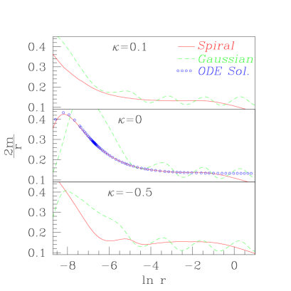
FIG. 1.: Critical solutions for both Gaussian (dashed, Eq. 2) and spiral (solid, Eq. 3) initial data for $\kappa=0.1,0.0,0.5$. The solution shown with open circles is that found by Hirschmann and Eardley with the assumption of continuous self-similarity [5].

Perturbations of this data are made according to

$$\psi(r,0) = f(r)~{}\left(A+\Delta A\right)~{}\cos\left(\omega r+\Delta\varphi\right)$$ (6)

$$\phi(r,0) = f(r)~{}A~{}\sin\left(\omega r\right),$$ (7)

and the critical solutions obtained are shown in Figs. 2 and 3. The figures show the last subcritical solution obtained by a critical search at a time just before it decides to disperse. The graphs then represent the outgoing record of the collapse of the self-similar regime towards $\ln r\rightarrow\infty$. Large $r$ then represents early time, and the graphs show that as the perturbation is increased, the self-similar pulse gradually develops a discrete oscillation. This development represents the funneling of the solution away from the CSS and toward the DSS.

These results make clear that changing the relative phase of the two fields or their relative amplitudes causes the critical solution to be attracted to the DSS. Perturbations of the relative frequency produces similar results.

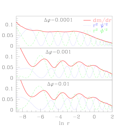
FIG. 2.: Perturbations of phase for the spiral initial data for $\kappa=0$. Even for small changes in the relative phase of $\psi$ and $\phi$, the critical solution is driven toward the DSS.

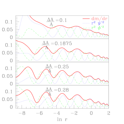
FIG. 3.: Perturbations of relative amplitude for the spiral initial data for $\kappa=0$. Again, the solution is driven toward the DSS.

While Figures 2 and 3 show that only initial data completely out of phase finds the CSS, the spiral data can be further perturbed via

$$F(r,0)=f(r)\exp\left(i\omega r^{p}\right)$$ (8)

for $p\neq 1$ and still be considered $\pi/2$ radians out of phase. However, as shown in Fig. 4, for $p\neq 1$ the CSS is not the critical solution. The initial data for these configurations are shown in Fig. 5.

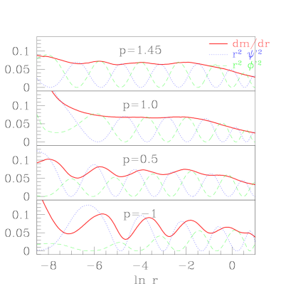
FIG. 4.: Critical solutions ($\kappa=0$) obtained for the spiral data for various values of $p$ [Eq. (8)]. The initial data for these critical solutions are shown in Figure 5.

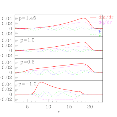
FIG. 5.: Initial data for the critical solutions displayed in Figure 4.

Before discussing these results, it is interesting to consider initial data which consists of the superposition of two different frequencies $\omega_{1}$ and $\omega_{2}$

$$F(r,0)=f_{1}(r)e^{i\omega_{1}r}+f_{2}(r)e^{i\omega_{2}r}.$$ (9)

Both the initial data and the critical solution are shown in Fig. 6. This example of the superposition of two frequencies finds the CSS as shown in the figure, however, not all examples of this family do. Families with $f_{1}=f_{2}$ and comparable frequencies resulted in critical solutions which appeared CSS.

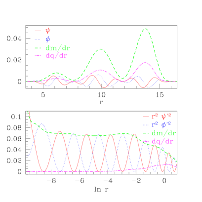
FIG. 6.: Critical solution obtained for initial data consisting of two frequencies $\omega_{1}=2.1$ and $\omega_{2}=3.6$ [Eq. (9)]. The top frame shows the initial data. The bottom frame displays the critical solution.

As mentioned previously, initial data which is otherwise spiral but has $f(r)$ varying on scales comparable to $\omega$ is driven away from the CSS critical solution in much the same way that the perturbations shown in Figures 2 and 3 drive the solution away from the CSS. Also, many examples of initial data of the form (9) are similarly driven away from the CSS. Experimentally, the strongest indicator of initial data which will find the CSS is when the energy density is everywhere proportional to the charge density. That this proportionality indicates the specialness of spiral initial data is discussed in Section III B.

III Discussion

Surprisingly enough, in this case a discussion of the DSS critical solution in the region $\kappa\gtrsim 0.1$ is simpler than the discussion of the CSS. In this region of parameter space, it is the DSS which has multiple unstable modes, and it is relatively easy to understand the families of initial data which find the DSS. Hence, the discussion of these special families is presented first, followed by a discussion of the specialness of the spiral data.

A The DSS

In the harmonic map model, for $\kappa\gtrsim 0.1$ the CSS is the attracting critical solution. Numerical evolutions of various families of initial data generically find the CSS, and do not find the DSS. Gundlach showed that the DSS has only one unstable mode for $\kappa=0$, but the stability analysis of the DSS has not been done for general $\kappa$ [7]. However, evolutions of this model, as well as results in the equivalent region of the model in [6], clearly indicate that for $\kappa\gtrsim 0.1$ the DSS has more than one unstable mode.

However, there are non-generic families that do find the DSS in this regime despite the presence of these extra unstable modes. Consideration of this phenomenon is helpful in understanding the CSS occurring for $\kappa=0$.

One description of initial data that finds the DSS in this regime is mentioned in [6]. In that work it was found that when one component of the field was initially vanishing, it remained zero. The model here, being equivalent to that one for $\kappa>0$, retains this feature as shown in the equations of motion for the two components of the scalar field in Equation (38). Because the CSS is necessarily complex (it has charge), initial data with one field initially vanishing is unable to find the CSS as its critical solution. Thus, families of initial data of the form

$$F(r) = f(r)$$ (10)

$$\psi(r) = f(r)$$ (11)

$$\phi(r) = 0$$ (12)

for arbitrary $f(r)$ will only find the DSS.

However, a more general set of families can be found with this principle in mind. Consider initial data of the form

$$F(r) = e^{iC}~{}f(r)$$ (13)

$$\psi(r) = \cos\left(C\right)f(r)$$ (14)

$$\phi(r) = \sin\left(C\right)f(r)$$ (15)

for arbitrary constant $C$. This data corresponds to a global rotation of Eq. (11) by an angle $C$ in the complex plane. Because the Lagrangian is invariant with respect to this rotation, the critical solution must be the same as the initial data described by Equation (11).

A more physical understanding of this can be gained by examining the issue of charge. For both sets of initial data (11,14), the charge is zero. In fact, all components of the current density, Equation (32), vanish

$$j_{\mu}=0.$$ (16)

The divergence of this current is zero, so the current density will not grow if initially vanishing. In other words, the system with no charge is in a symmetric state with respect to charge, and this symmetry would have to be broken were the charge to become positive or negative.

Because the CSS can have either positive or negative charge, these sets of initial data are precisely balanced between trajectories that would take them to the CSS with positive charge and those that would take them to the negatively charged CSS (since the model is independent of which field is considered the imaginary component and which the real component of the complex scalar field, the sign of the charge of the CSS is arbitrary). It is this balance that enables them to see the DSS as a critical solution with only one unstable mode when in fact it has more than one. The initial data has already tuned one of the extra unstable modes (or an unstable conjugate pair of modes).

With the knowledge that the extra unstable mode corresponds to a charged mode, a two-parameter search can now be conducted. Determination of an appropriately parameterized initial data family is somewhat more subtle than that for the one parameter data. With a one parameter search, a parameterization needs to be smooth and monotonic in the mass of the initial data near the critical point because the excitation of the black hole mode is characterized by the mass contained. Here, that mode must also be tuned, but the unstable charged modes must be tuned as well. Hence, the second parameter must be locally monotonic in charge near the critical point.

A two parameter search with the data

$$f(R) = e^{-\left(r-R\right)^{2}/D^{2}}$$ (17)

$$\psi(r) = p~{}f(R_{\psi})$$ (18)

$$\phi(r) = p~{}f(R_{\psi}-\delta+10p)$$ (19)

finds the DSS. Here, $f(R)$ is a Gaussian pulse centered on some radius $R$, and $R_{\psi}$ and $D$ are arbitrary constants. The parameters $p$ and $\delta$ are used to tune both the mass and the charge of the initial data. For $\delta$ fixed, $p$ effectively tunes the initial energy content. With $p$ fixed and with $\delta\approx 10p$, increasing $\delta$ increases the charge from some negative value up to some positive value (the constant $10$ is chosen arbitrarily). Setting $\delta=10p$ turns the family back into one with zero charge.

With this data, some value for $\delta$ near the value $10p$ is chosen, and the black hole critical solution is bracketed sufficiently closely so that the sign of the initial charge of the critical solution is known. A different $\delta$ is chosen so that the sign of the charge of the critical solution is found to be the opposite sign. These two values of $\delta$ then bracket a critical value $\delta^{*}$ for which the critical solution ($p=p^{*}$) has zero charge. In this manner, the DSS is found.

The difference between this two-parameter tuning and using initial data with zero charge is simply the order in which the tuning occurs. In the latter, the initial data is already tuned to have zero charge. The remaining task is then to tune the mass. However in the former, the charge is being tuned first to arrive at a one-parameter family that in general has charge. It is only at the critical value of $p$ that this one-parameter family (found from the $\delta$ search) that the solution has zero charge.

In Figure 7 a series of critical solutions for $\kappa=1$ with initial data of the form (18) are shown. For each case, $|p-p^{*}|$ is of order machine precision. The critical solution gets closer to the DSS in the limit $\left(\delta-\delta^{*}\right)/\delta^{*}\rightarrow 0$. Interestingly, while the critical solutions of the perturbed spiral data in Figure 3 appeared initially to be headed toward the CSS only to be funneled to the DSS, these solutions do the opposite. They begin initially as DSS solutions but eventually head to the CSS. As they get closer to the critical solution $\delta^{*}$, the DSS lasts for a progressively longer time. This similarity is consistent with the spiral being tuned to the unstable modes of the CSS.

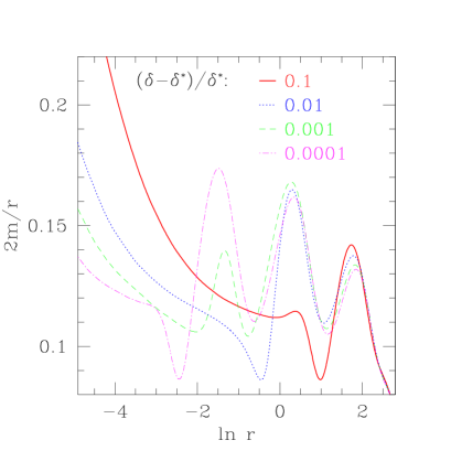
FIG. 7.: Critical solutions with $\kappa=1$ for various levels of charge tuning $\left(\delta-\delta^{*}\right)/\delta^{*}$. The initial data is of the form found in Eq (18). The field $2m/r$ is shown for $\left(\delta-\delta^{*}\right)/\delta^{*}$ equal to ${0.1,0.01,0.001,0.0001}$. As $\delta$ approaches $\delta^{*}$ the solution appears discretely self-similar longer but eventually becomes the CSS.

B The CSS

Initial data of the form Equation (14) will always find the DSS, because, having no charge, a direction must be picked toward either positive or negative charge to break the symmetry. In the case of finding the multiply-unstable CSS, the spiral data maximizes the charge of the initial data for a given energy, and so it appears that a symmetry must be broken to disperse all the charge and arrive at the DSS.

To find a bound on the charge, consider the norm of the vector $\left[F^{a}F^{a}F^{c}_{,\mu}\pm\frac{\left(1-\kappa|F|^{2}\right)^{2}}{2}\epsilon_{cd}F^{d}j_{\mu}\right]$ at the initial time for time-symmetric initial data. Because at the initial time all the time components vanish, the norm is positive definite. This is similar to a trick employed by Belavin and Polyakov [8] and described in Rajaraman [9]. Computing

$$\left[F^{a}F^{a}F^{c}_{,\mu}\pm\frac{\left(1-\kappa|F|^{2}\right)^{2}}{2}\epsilon_{cd}F^{d}j_{\mu}\right]~{}~{}~{}~{}~{}~{}~{}~{}~{}~{}~{}~{}~{}~{}~{}~{}$$ (20)

$$\times\left[F^{a}F^{a}F^{c}{}^{,\mu}\pm\frac{\left(1-\kappa|F|^{2}\right)^{2}}{2}\epsilon_{ce}F^{e}j^{\mu}\right] \geq 0$$ (21)

$$|F|^{2}F_{,\mu}F^{*}{}^{,\mu}\geq\frac{\left(1-\kappa|F|^{2}\right)^{4}}{4}j_{\mu}j^{\mu}.$$ (22)

This inequality (22) can be expressed in terms of the energy density for time-symmetric initial data

$$T_{00}=\frac{\alpha^{2}F_{,\mu}F^{*}{}^{,\mu}}{8\pi\left(1-\kappa|F|^{2}\right)^{2}}.$$ (23)

The bound is then

$$\frac{32\pi|F|^{2}}{\left(1-\kappa|F|^{2}\right)^{2}}T_{00}\geq\alpha^{2}j_{\mu}j^{\mu}$$ (24)

which, for $\kappa=0$, is simply

$$32\pi|F|^{2}T_{00}\geq\alpha^{2}j_{\mu}j^{\mu}.$$ (25)

Hence there is an upper limit to the square of the charge density for a given energy density.

Letting the initial data be of the general form (3), the condition to saturate this bound for $\kappa=0$ is

$$|F|^{2}F_{,\mu}F^{*}{}^{,\mu}=\frac{1}{4}j^{\mu}j_{\mu}$$ (26)

which implies

$$\left(f^{\prime}\right)^{2}=0.$$ (27)

Saturation therefore occurs when all energy occurs in the phase rotation, $h^{\prime}$. Physically, this is apparent by looking at the behavior of $F$ in the complex plane. Because $f^{\prime}$ vanishes, as $F$ is traced out for various $r$, the magnitude $f$ does not change; only the phase is changing so the path is a circle on the plane. This tracing then maximizes the area covered for a given energy. The area covered is proportional to the charge, so the charge is maximized.

This analysis applies only for $\kappa=0$ with time-symmetric initial data, though presumably similar arguments would hold for the generalization to other values of $\kappa$ and ingoing initial data.

At this point, it is interesting to compare the family (14) to the spiral initial data. These two families are, in some sense, complementary. Pick some $r$, and imagine that point in the complex plane. To construct data of the form (14), determine the field values for all other $r$ by requiring these points to fall on the radial line between this initial point and the origin. In this fashion, the initial data will have some global phase, constant in $r$, equal to some value $C$. However beginning once again from that initial point in the plane, the restriction of Equation (27) says that to construct spiral initial data, as $r$ is increased the curve in the plane must lie everywhere perpendicular to the radial direction.

Another condition restricting the spiral data appears to be that the charge density must be independent of $r$. Just as seen with families that find the multiply unstable DSS where the charge density must be everywhere zero independent of $r$, here the charge density must be everywhere a maximum and independent of $r$.

In order for the charge density to be independent of $r$, the rate at which the data covers the plane, $\omega=h^{\prime}$, must be constant in $r$. Initial data which would otherwise be spiral but with $h^{\prime}\neq 0$ are shown in Figure 5 with their respective critical solutions shown in Figure 4. These results indicate that only for $p=1$ in Equation (8) is the CSS found.

Another perspective on the constraints of the spiral data is afforded by examining the ratio of the charge density to the energy density

$$\frac{j_{\mu}}{F_{,\mu}F^{*}{}^{,\mu}}=\frac{2a^{2}f^{2}h^{\prime}}{\left(f^{\prime}\right)^{2}+f^{2}\left(h^{\prime}\right)^{2}}=\frac{2a^{2}}{h^{\prime}}.$$ (28)

That this ratio is approximately independent of $r$ for the conditions $f^{\prime}=0$ and $h^{\prime\prime}=0$ appears to indicate that tuning the mass of the initial data also tunes the charge. In other words, with the charge to mass ratio everywhere the same, the critical search cannot find a solution which disperses all the charge.

Construction of smooth, compact, and regular initial data consistent with the restrictions

$$f^{\prime}(r,0)=0~{}~{}~{}~{}~{}~{}~{}h^{\prime\prime}(r,0)=0$$ (29)

is quite difficult. Regularity at the origin requires either $f(0,t)=0$ or $f^{\prime}(0,t)=0=h^{\prime}(0,t)$.

Satisfying the former along with strict observance of (29) leads to the trivial solution $F(r,0)=0$. Instead, as mentioned earlier, initial data is used where $f$ vanishes at the origin, but is then “turned on” at some larger $r$. The condition $f^{\prime}=0$ is then not satisfied everywhere, but for $f^{\prime}\ll\omega$ the CSS is still found.

Satisfying the latter condition along with $h^{\prime\prime}=0$ at the initial time also leads to a trivial solution $F(r,0)=C$, for some complex constant $C$. Again, $\omega$ can be “turned on” at some larger $r$, but this can only be done in a smooth way if $h^{\prime\prime}(r,0)$ is not everywhere zero.

The difficulty in constructing non-trivial, regular, initial data which is strictly spiral has hampered the analysis. While initial data of the form (14) has the symmetry $\phi(r)=\tan\left(C\right)\psi(r)$ which holds at all times, it is not clear if there is such a preserved symmetry here. The approximate symmetry $\phi(r)=\tan\left(\omega r\right)\psi(r)$ holds at the initial time for the spiral data but does not appear to hold throughout the evolution. Also, the bound (27) is shown only for time-symmetric initial data but ingoing spiral data also finds the CSS. However, the evolutions consistently show that initial data which has the ratio of charge density to energy density independent of $r$ will find the CSS as its critical solution.

IV Conclusion

A special family of initial data is described which finds the CSS critical solution in a region of parameter space where generic initial data finds the DSS. The specialness of this family is discussed. A bound on the charge density for time-symmetric initial data is found, which this family saturates. Because the spiral data maximizes the charge density and because this charge density is independent of $r$, it is argued that the extra unstable modes cannot grow because their growth would pick a direction in which to decrease the charge. The inability of the extra modes to grow then indicates that the spiral data “see” only the black hole mode around the CSS.

Because both the CSS and DSS can both be found where they have multiple unstable modes, it seems possible that other suitably tuned families in other models might find other, previously unknown multiply unstable critical solutions.

Equations of Motion

The action $S$ for the model under study here is

$$S=\int d^{4}x\sqrt{-g}\left(R-\frac{2|\nabla F|^{2}}{\left(1-\kappa|F|^{2}\right)^{2}}\right),$$ (30)

defined in terms of a complex scalar field $F(r,t)$

$$F(r,t)=\psi(r,t)+i\phi(r,t),$$ (31)

its complex conjugate $F^{*}(r,t)$, and a dimensionless parameter $\kappa$. The operator $\nabla$ represents the covariant derivative. The action (30) is invariant with respect to global rotations of $F$, and thus has a conserved current

$$j_{\mu}=\frac{i\left(FF^{*}{}_{,\mu}-F^{*}F_{,\mu}\right)}{\left(1-\kappa|F|^{2}\right)^{2}}.$$ (32)

In component form where Latin indices run over $1$ and $2$ for the real and imaginary components, this current is

$$j_{\mu}=\frac{2}{\left(1-\kappa|F|^{2}\right)^{2}}\epsilon_{ab}F^{a}F^{b}{}_{,\mu}.$$ (33)

The field equations are then

$$G_{\mu\nu} = 8\pi T_{\mu\nu}$$ (34)

$$\Box F = \frac{-2\kappa F^{*}}{1-\kappa|F|^{2}}F_{;\mu}F^{;\mu}$$ (35)

where $G_{\mu\nu}$ is the usual Einstein tensor and the stress energy takes the form

$$T_{\mu\nu}=\frac{\psi_{,\mu}\psi_{,\nu}+\phi_{,\mu}\phi_{,\nu}-\frac{1}{2}g_{\mu\nu}\left(\psi_{,\rho}\psi^{,\rho}+\phi_{,\rho}\phi^{,\rho}\right)}{4\pi(1-\kappa\left(\psi^{2}+\phi^{2}\right))^{2}}.$$ (36)

In terms of the real and imaginary parts of $F$, the wave equation becomes

$$\Box\psi = -\frac{2\kappa\left[\psi\psi_{,\mu}\psi^{,\mu}-\psi\phi_{,\mu}\phi^{,\mu}+2\phi\psi_{,\mu}\phi^{,\mu}\right]}{1-\kappa\left(\psi^{2}+\phi^{2}\right)}$$ (37)

$$\Box\phi = -\frac{2\kappa\left[\phi\phi_{,\mu}\phi^{,\mu}-\phi\psi_{,\mu}\psi^{,\mu}+2\psi\psi_{,\mu}\phi^{,\mu}\right]}{1-\kappa\left(\psi^{2}+\phi^{2}\right)}.$$ (38)

We work in spherically symmetry with the metric

$$ds^{2}=-\alpha^{2}(r,t)dt^{2}+a^{2}(r,t)dr^{2}+r^{2}d\Omega^{2}.$$ (39)

We introduce the following auxiliary variables in order to cast the field equations in first order in time form

$$\Pi_{\psi}\equiv\frac{a}{\alpha}\dot{\psi} \Phi_{\psi}\equiv\psi^{\prime}$$ (40)

$$\Pi_{\phi}\equiv\frac{a}{\alpha}\dot{\phi} \Phi_{\phi}\equiv\phi^{\prime},$$ (41)

where overdots and primes denote derivatives with respect to $t$ and $r$, respectively. The two second order wave equations become four, first order equations

$$\dot{\Pi}_{\psi} = r^{-2}\left(\frac{r^{2}\alpha}{a}\Phi_{\psi}\right)^{\prime}$$ (42)

$$+ \frac{2\alpha\kappa\left[\psi\left(\Phi^{2}_{\psi}-\Pi_{\psi}^{2}-\Phi^{2}_{\phi}+\Pi_{\phi}^{2}\right)+2\phi\left(\Phi_{\psi}\Phi_{\phi}-\Pi_{\psi}\Pi_{\phi}\right)\right]}{a\left(1-\kappa\left(\psi^{2}+\phi^{2}\right)\right)}$$ (43)

$$\dot{\Phi}_{\psi} = \left(\frac{\alpha}{a}\Pi_{\psi}\right)^{\prime}$$ (44)

$$\dot{\Pi}_{\phi} = r^{-2}\left(\frac{r^{2}\alpha}{a}\Phi_{\phi}\right)^{\prime}$$ (45)

$$+ \frac{2\alpha\kappa\left[\phi\left(\Phi^{2}_{\phi}-\Pi_{\phi}^{2}-\Phi^{2}_{\psi}+\Pi_{\psi}^{2}\right)+2\psi\left(\Phi_{\phi}\Phi_{\psi}-\Pi_{\phi}\Pi_{\psi}\right)\right]}{a\left(1-\kappa\left(\psi^{2}+\phi^{2}\right)\right)}$$ (46)

$$\dot{\Phi}_{\phi} = \left(\frac{\alpha}{a}\Pi_{\phi}\right)^{\prime}.$$ (47)

The fields $\psi$ and $\phi$ are maintained at each time step by spatially integrating their respective spatial derivatives

$$\psi(r,t) = \int_{0}^{r}\Phi_{\psi}(\tilde{r},t)~{}d\tilde{r}$$ (48)

$$\phi(r,t) = \int_{0}^{r}\Phi_{\phi}(\tilde{r},t)~{}d\tilde{r}.$$ (49)

The Hamiltonian constraint is

$$\frac{a^{\prime}}{a}+\frac{a^{2}-1}{2r}=\frac{r\left[\Phi^{2}_{\psi}+\Phi^{2}_{\phi}+\Pi_{\psi}^{2}+\Pi_{\phi}^{2}\right]}{2(1-\kappa\left(\psi^{2}+\phi^{2}\right))^{2}}.$$ (50)

The nature of polar slicing and the radial gauge yields the constraint on the lapse function $\alpha$

$$0=\frac{\alpha^{\prime}}{\alpha}-\frac{a^{\prime}}{a}+\frac{1-a^{2}}{r}.$$ (51)

Finally, combination of an evolution equation and a momentum constraint yields an evolution equation for $a$

$$\dot{a}=r\alpha\frac{\Phi_{\psi}\Pi_{\psi}+\Phi_{\phi}\Pi_{\phi}}{(1-\kappa\left(\psi^{2}+\phi^{2}\right))^{2}}.$$ (52)

Regularity of the solution at the origin demands

$$a(0,t)^{\prime} = \alpha(0,t)^{\prime}=0$$ (53)

$$\Phi_{\psi}(0,t) = \Phi_{\phi}(0,t)=0,$$ (54)

and local flatness there is enforced by

$$a(0,t)=1.$$ (55)

We have the freedom to pick a condition on $\alpha$ on each time slice which corresponds to a global change in the labeling of slices. We impose the condition on $\alpha$ at the large radius boundary of the grid $r_{\rm max}$

$$\alpha(r_{\rm max},t)=\frac{1}{a(r_{\rm max},t)}.$$ (56)

As long as no radiation is escaping from the grid, this condition implies that coordinate time $t$ corresponds to proper time for an observer at $r=\infty$.

The nature of being restricted to a finite grid imposes the need for an artificial boundary condition on the matter fields there. Since our spacetime is asymptotically flat, we impose an approximate outgoing radiation condition on the matter fields. The flat space wave equation for some general scalar field $\Theta(r,t)$ in spherical symmetry

$$\Box\Theta\Rightarrow\left(r\Theta\right)_{tt}=\left(r\Theta\right)_{rr}$$ (57)

has the solution

$$r\Theta=f(r+t)+g(r-t)$$ (58)

for two general functions $f$ (in-going component) and $g$ (out-going component). To eliminate the in-going component at the outer boundary, we enforce at the boundary the condition

$$\frac{\partial\left(r\Theta\right)}{\partial r}=-\frac{\partial\left(r\Theta\right)}{\partial t}$$ (59)

with the equations

$$\dot{\Pi}_{\Theta}+\Pi_{\Theta}^{\prime}+\frac{\Pi_{\Theta}}{r} = 0$$ (60)

$$\dot{\Phi}_{\Theta}+\Phi_{\Theta}^{\prime}+\frac{\Phi_{\Theta}}{r} = 0,$$ (61)

which effectively limits reflection off the outer boundary.

The metric (39) corresponds to a “dynamical” Schwarzschild metric, allowing the association

$$a^{2}(r,t)=\left(1-\frac{2m(r,t)}{r}\right)^{-1},$$ (62)

where the field $m(\tilde{r},\tilde{t})$ represents the mass aspect function measuring the amount of mass contained within a shell of radius $\tilde{r}$ centered about the origin at coordinate time $\tilde{t}$. Eq. (62) leads to

$$m(r,t)=\frac{r}{2}\left(1-\frac{1}{a^{2}}\right),$$ (63)

so that from the field $a(r,t)$, we can obtain the mass aspect function.

An advantage of polar slicing (and most slicing conditions used in numerical relativity) is that it avoids singularities. Further, because of our use of polar-areal coordinates, we cannot observe the formation of a true horizon which is a coordinate singularity in our coordinates. Instead, by monitoring $m(r,t)/r$ we can observe the formation of a horizon and hence a black hole when $m/r\rightarrow 1/2$. Where $m/r$ approaches $1/2$, we can determine the mass of the black hole forming by simply halving the radius where the horizon forms.

REFERENCES

- [1] M.W. Choptuik, Phys. Rev. Lett., 70, 9-12 (1993).
- [2] A.M. Abrahams and C.R. Evans, Phys Rev. Lett., 70, 2980-2983 (1993).
- [3] C.R. Evans and J.S. Coleman, Phys Rev. Lett., 72, 1782-1785 (1994).
- [4] D. Maison, Phys. Lett. B366, 82-84 (1996), gr-qc/9504008.
- [5] E.W. Hirschmann and D.M. Eardley, Phys. Rev. D56, 4696-4705 (1997), gr-qc/9511052.
- [6] S.L. Liebling and M.W. Choptuik, Phys. Rev. Lett. 77, 1424-1427 (1996), gr-qc/9606057.
- [7] C. Gundlach, Phys. Rev. Lett. 75, 3214-3217 (1995), gr-qc/9507054.
- [8] A.A. Belavin and A.M. Polyakov, JETP Lett. 22, 245 (1975).
- [9] R. Rajaraman, Solitons and Instantons (North Holland Pub., New York, 1982).