gr-qc/9805037

April 23, 1998

Quantum Inequality Restrictions on Negative
Energy Densities in Curved Spacetimes

A dissertation submitted by

Michael John Pfenning
In partial fulfillment of the requirements

for the degree of Doctor of Philosophy in the

Department of Physics and Astronomy,

TUFTS UNIVERSITY

Medford, Massachusetts 02155

Advisor: Lawrence H. Ford

Abstract

In quantum field theory, there exist states in which the expectation value of the energy density for a quantized field is negative. These negative energy densities lead to several problems such as the failure of the classical energy conditions, the production of closed timelike curves and faster than light travel, violations of the second law of thermodynamics, and the possible production of naked singularities.

Although quantum field theory introduces negative energies, it also provides constraints in the form of quantum inequalities (QI’s). These uncertainty principle-type relations limit the magnitude and duration of any negative energy. We derive a general form of the QI on the energy density for both the quantized scalar and electromagnetic fields in static curved spacetimes. In the case of the scalar field, the QI can be written as the Euclidean wave operator acting on the Euclidean Green’s function. Additionally, a small distance expansion on the Green’s function is used to derive the QI in the short sampling time limit. It is found that the QI in this limit reduces to the flat space form with subdominant correction terms which depend on the spacetime geometry.

Several example spacetimes are studied in which exact forms of the QI’s can be found. These include the three- and four-dimensional static Robertson-Walker spacetimes, flat space with perfectly reflecting mirrors, Rindler and static de Sitter space, and the spacetime outside a black hole. In all of the above cases, we find that the quantum inequalities give a lower limit on how much negative energy may be observed relative to the vacuum energy density of the spacetime. For the particular case of the black hole, it is found that the quantum inequality on the energy density is measured relative to the Boulware vacuum.

Finally, the application of the quantum inequalities to the Alcubierre warp drive spacetime leads to strict constraints on the thickness of the negative energy region needed to maintain the warp drive. Under these constraints, we discover that the total negative energy required exceeds the total mass of the visible universe by a hundred billion times, making warp drive an impractical form of transportation.

Acknowledgments

There are many people to whom I would like to express my gratitude. First and foremost is my advisor and mentor, Dr. Lawrence H. Ford. Without his encouragement, patience and support, I would never have been able to complete this dissertation. A special thanks also goes to Dr. Thomas A. Roman for his unfailing advice and encouragement. I also wish to thank Dr. Allen Everett for all of the input over the course of my research. The Institute of Cosmology and the Department of Physics at Tufts University also deserve credit for making all of my research possible. I would also like to thank all of the people in the Department Office who’s humor and assistance were invaluable.

On a more personal level, an extra special thank you goes to Dorothy Drennen, who gave up her personal time to edit this manuscript from cover to cover. The same heart felt gratitude goes to Vicki Ford, who was also there to keep me on course. Finally, I would like to thank my family for all of their love throughout the years. A special wish goes to my two sons, Henry and René, who have brought so much joy into my life. To Fran, Herbert, Heidi, John, and my Grandmother Mary, I dedicate this manuscript.

The financial support of NSF Grant No. Phy-9507351 and the John F. Burlingame Physics Fellowship Fund is gratefully acknowledged.

Chapter 1 Energy Conditions in General Relativity

1.1 The Classical Energy Conditions

The most powerful and intriguing tool in cosmology is Einstein’s equation,

$$G_{\mu\nu}\equiv R_{\mu\nu}-{1\over 2}Rg_{\mu\nu}=8\pi GT_{\mu\nu}.$$ (1.1)

Here we have chosen the spacetime metric to have a $(-,+,+,+)$ signature and the definitions of the Riemann and Ricci tensors in the convention of Misner, Thorne and Wheeler [1]. Einstein’s equation relates the spacetime geometry on the left with the matter source terms on the right. The equation is interesting in that it admits a large number of solutions. If there are no physical constraints on the metric or the stress-tensor, then Einstein’s equation is vacuous since any metric would be a “solution” corresponding to some distribution of the stress-energy. We could then have “designer spacetimes” which could exhibit any behavior that one likes. Therefore, if we can place any limitations upon the equation, or on terms in the equation, we could limit the search for physically realizable solutions.

The most trivial condition comes from the Bianchi identities, that the covariant divergence of the Einstein tensor must vanish:

$$\nabla_{\mu}G^{\mu\nu}=0.$$ (1.2)

From Einstein’s equation, this leads to the condition on the stress-energy tensor of

$$\nabla_{\mu}T^{\mu\nu}=0.$$ (1.3)

This is the covariant form of the conservation of energy in general relativity.

The next condition which is generally considered reasonable for all classical matter is that the energy density seen by an observer should be non-negative. Consider an observer who moves along the geodesic $\gamma^{\mu}(\tau)$. Then his four-velocity,

$$u^{\mu}(\tau)\equiv{d\over d\tau}\gamma^{\mu}(\tau),$$ (1.4)

is everywhere timelike and tangent to the curve $\gamma^{\mu}(\tau)$. In the observer’s frame, the statement that the energy density should be non-negative is

$$T_{\mu\nu}u^{\mu}(\tau)u^{\nu}(\tau)\geq 0,\qquad\mbox{ for all timelike }u^{\nu}(\tau).$$ (1.5)

This is typically called the Weak Energy Condition (WEC). This condition was an important assumption in the proof of the singularity theorem developed by Penrose [2]. In the early part of this century, it was known that a spherically symmetric object that underwent gravitational collapse would form a black hole, with a singularity at the center. However, relativists were unsure if the same would be true for a more generic distribution of matter. Penrose’s original singularity theorem showed that the end product of gravitational collapse would always be a singularity without assuming any special symmetries of the matter distribution. The WEC is used in the proof of the singularity theorem in the Raychaudhuri equation to ensure focusing of a congruence of null geodesics. An additional assumption sometimes used in the proof of the singularity theorems is the Strong Energy Condition (SEC),

$$\left(T_{\mu\nu}-{1\over 2}Tg_{\mu\nu}\right)u^{\mu}(\tau)u^{\nu}(\tau)\geq 0,\qquad\mbox{ for all timelike }u^{\nu}(\tau).$$ (1.6)

Here $T={T_{\mu}}^{\mu}$ is the contraction of the stress-tensor. If the SEC is satisfied, then it ensures that gravity is always an attractive force. The SEC is “stronger” than the WEC only in the sense that it is a more restrictive condition, and therefore it is much easier to violate the SEC than the WEC.

Immediately following the successes of Penrose’s singularity theorem for black holes, Hawking [3, 4] developed a similar theorem for the open Friedman-Robertson-Walker universe which showed that there had to exist an essential, initial singularity from which the universe was born. Nearly thirty years later, singularity theorems are still being proven for various spacetimes. For example, Borde and Vilenkin have proven the existence of initial singularities for inflationary cosmologies and for certain classes of closed universes [5, 6].

For completeness, we also mention two other classical energy conditions. The first is the Null Energy Condition (NEC),

$$T_{\mu\nu}K^{\mu}K^{\nu}\geq 0,\qquad\mbox{ for all }K^{\nu},$$ (1.7)

where $K^{\mu}$ is the tangent to a null curve. The NEC follows by continuity from both the WEC (1.5) and the SEC (1.6) in the limit when $u^{\mu}$ becomes a null vector. The second condition is a little different from the previous ones. Let us assume, as we did above, that $u^{\nu}$ is a future-directed timelike vector. It follows that the product, $-{T^{\mu}}_{\nu}u^{\nu}$, should also be a future-directed timelike or null vector. This is known as the Dominant Energy Condition (DEC) and can be interpreted to mean that the speed of energy flow of matter should always be less than the speed of light.

We see that the energy conditions at the classical level are an extremely useful tool that have yielded some remarkable results in the form of the singularity theorems and positive mass theorems. However, many of the energy conditions are doomed to failure when quantum field theoretic matter is introduced as the source of gravity. A first approximation to a “quantum theory of gravity” is achieved via the semiclassical equation

$$G_{\mu\nu}=8\pi G\langle T_{\mu\nu}\rangle.$$ (1.8)

We are still treating the spacetime as a “smooth” classical background, but we have replaced the classical stress-tensor with its renormalized quantum expectation value. It is presumed that the field equation should be valid in the test field limit where the mass and/or the energy of the quantized field is not so large as to cause significant back-reaction on the spacetime. However, the replacement of the classical stress-tensor with its quantum expectation value is not without difficulty. At the same time that Penrose and Hawking were introducing the singularity theorems, Epstein, Glaser and Jaffe [7] were demonstrating that the local energy density in a quantized field theory was not always positive definite. We will see in Chapter 2 that it is possible to construct specific quantum states in which the energy density is negative along some part of an observer’s worldline. The simplest example, discussed in Section 2.1, is a state in which the particle content of the theory is a superposition of the vacuum plus two particle state. Another example is the squeezed states of light which have been produced and observed experimentally [8], although it is unclear at this time whether it is possible to measure the negative energy densities that exist for these two cases. However, there is the interesting case of the Casimir vacuum energy density for the quantized electromagnetic field between two perfectly conducting parallel plates [9]. Here the vacuum energy between the plates is found to be a constant and everywhere negative. Indirect effects of the negative vacuum energy, in the form of the Casimir force which causes the plates to be attracted to one another, has been measured experimentally [10, 11]. It has even been suggested that the Casimir force may play a role in the measurement limitations in electron force microscopy [12].

Related to the Casimir vacuum energy is the vacuum energy of a quantized field in curved spacetime, which we will discuss further in Section 2.3. An example is the static closed universe, where the vacuum energy for the conformally coupled field is positive [13, 14], while that of the minimally coupled field is negative [15]. Instances of non-zero vacuum energies in the semiclassical theory of gravity seem to be extremely widespread. The most well known, and probably most carefully studied, is the vacuum energy around a black hole. Hawking has shown that this causes the black hole to evaporate, with a flux of positive energy particles being radiated outward. In this case both the WEC and the NEC are violated [16, 17, 18, 19, 20, 21, 22].

In terms of a consistent mathematical theory of semiclassical gravity, the existence of negative energy densities is not necessarily a problem. On the contrary, it could be viewed as beneficial because it would allow spacetimes in which time travel would be possible, or where mankind could construct spacecraft which could warp spacetime around them in order to travel around the universe faster than the speed of light. Even wormholes would be allowed as self-consistent solutions to Einstein’s equation.

Objections to negative energies are raised for several reasons such as violations of the second law of thermodynamics, the possibility of creating naked singularities by violating cosmic censorship, and the loss of the positive mass theorems. On the more philosophical side, if time travel, space or time warps, wormholes and any other exotic solution that physicists can dream up were allowed, then we would have to deal with a new set of complexities, such as problems with causality and the notion of free will. Visser’s [23] description of four possible schools of thought on how to build an entirely self-consistent theory of physics with regard to time travel is quoted here:

1. The radical rewrite conjecture: One might make one’s peace with the notion of time travel and proceed to rewrite all of physics (and logic) from the ground up. This is a very painful procedure, not to be undertaken lightly.

2. Novikov’s consistency conjecture: This is a slightly more modest way of making one’s peace with the notion of time travel. One simply asserts that the universe is consistent, so that whatever temporal transpositions and trips one undertakes, events must conspire in such a way that the overall result is consistent. (A more aggressive version of the consistency conjecture attempts to derive this “principle of self-consistency” from some appropriate micro-physical assumptions.)

3. Hawking’s chronology protection conjecture: Hawking has conjectured that the cosmos works in such a way that time travel is completely and utterly forbidden. Loosely speaking, “thou shalt not travel in time,” or “suffer not a time machine exist.” The chronology protection conjecture permits spacewarps/wormholes but forbids timewarps/time machines.

4. The boring physics conjecture: This conjecture states, roughly: “A pox upon all nonstandard speculative physics. There are no wormholes and/or spacewarps. There are no time machines/timewarps. Stop speculating. Get back to something we know something about.”

Besides the philosophical reasons, there is one particularly important mathematical result of the classical theory of gravity that would fail if negative energies did exist and were widespread. These are the singularity theorems which establish the existence of singularities in general relativity, particularly for gravitational collapse and at the initial “big bang.”

1.2 The Averaged Energy Conditions

In the 1970’s and 1980’s, several approaches were proposed to study the extent to which quantum fields may violate the weak energy condition, primarily with the hope of restoring some, if not all, of the classical general relativity results. In 1978, Tipler suggested averaging the pointwise conditions over an observer’s geodesic [24]. Subsequent work by various authors [25, 26, 27, 28, 29, 30, 31] eventually led to what is presently called the Averaged Weak Energy Condition (AWEC),

$$\int_{-\infty}^{\infty}\langle T_{\mu\nu}u^{\mu}u^{\nu}\rangle d\tau\geq 0,$$ (1.9)

where $u^{\mu}$ is the tangent to a timelike geodesic and $\tau$ is the observer’s proper time. Here the energy density of the observer is not measured at a single point, but is averaged over the entire observer’s worldline. Unlike the WEC, the AWEC allows for the existence of negative energy densities so long as there is compensating positive energy elsewhere along the observer’s worldline.

There is also an Averaged Null Energy Condition (ANEC),

$$\int_{-\infty}^{\infty}\langle T_{\mu\nu}K^{\mu}K^{\nu}\rangle d\lambda\geq 0,$$ (1.10)

where $K^{\mu}$ is the tangent to a null geodesic, and $\lambda$ is the affine parameter along that null curve. Roman [28, 29] has demonstrated in a series of papers that the singularity theorem developed by Penrose will still hold if the weak energy condition is replaced by the averaged null energy condition. Therefore, within the limits of the semiclassical theory there exists the possibility of recovering some, if not all, of the classical singularity theorems.

The ANEC is somewhat unique in that it follows directly from quantum field theory. Wald and Yurtsever [31] showed that the ANEC could be proven to hold in two dimensions for any Hadamard state along a complete, achronal null geodesic. They also showed that the same result held in four-dimensional Minkowski spacetime as well. The results in two-dimensional flat spacetime were confirmed by way of an entirely different method by Ford and Roman [32]. The question of whether back-reaction would enforce the averaged null energy condition in semiclassical gravity has been addressed recently by Flanagan and Wald [33]. Their work seems to indicate that if violations of the ANEC do occur for self-consistent solutions of the semiclassical equations, then they cannot be macroscopic, but are limited to the Planck scale. On such a tiny scale, we do not know if the semiclassical theory is reliable. It is expected that at the Planck scale the effects of a full quantum theory of gravity would be important.

At first the averaged energy conditions seem like a vast improvement. If the averaged energy conditions hold in general spacetimes, there is hope that we can restore the singularity theorems and gain a new class of energy conditions better suited for dealing with quantum fields. However, it is straightforward to show that both the AWEC and the ANEC are violated for any observer when the quantum field is in the vacuum state in certain spacetimes. The simplest example is an observer who sits at rest between two uncharged, perfectly conducting plates. Casimir [9] showed for the quantized electromagnetic field that the vacuum energy between the plates is negative. Therefore, over any time interval which we average, the AWEC will fail. Similar effects can occur in curved spacetime for the vacuum state. Examples are the various vacuum states outside a black hole [17, 18, 19, 20, 21, 22]. It appears that a difference between an arbitrary state and the vacuum state often obeys a type of AWEC, which can be written as

$$\int_{-\infty}^{\infty}\left[\langle\psi|T_{\mu\nu}u^{\mu}u^{\nu}|\psi\rangle-\langle 0_{c}|T_{\mu\nu}u^{\mu}u^{\nu}|0_{c}\rangle\right]d\tau\geq 0.$$ (1.11)

This equation, which has been called the Quantum Averaged Weak Energy Condition (QAWEC) is derived in Section 3.2. It holds for a certain class of observers in any static spacetime [32, 34, 35, 36] and is the result of the infinite sampling time limit of the quantum inequalities, which will be defined below.

Another aspect of the averaged energy conditions is that there are a number of “designer” spacetimes where they are necessarily violated. Three examples of particular interest are: the traversable wormhole [37, 38], the Alcubierre “warp drive” [39, 40], and the Krasnikov tube [41, 42]. All three require negative energy densities to maintain the spacetime. Likewise, all three have similar problems in that slight modifications of these spacetimes would lead to closed timelike curves, and would allow backward time travel [43]. Thus, these spacetimes may be entirely unphysical in the first place. It has also been shown by various researchers that if warp drives and wormholes exist, then they must be limited to the Planck size [40, 42, 44]; otherwise extreme differences in the scales which characterize them would exist. In Chapter 5 we will discuss the example of the macroscopic warp drive, where we find that the warp bubble’s radius can be on the order of tens or hundreds of meters, but the bubble’s walls are constrained to be near the Planck scale. Similar results have been found for wormholes and the Krasnikov tube.

There is also a limitation in the averaged energy conditions. The AWEC and the ANEC say nothing about the distribution or magnitude of the negative energy that may exist in a spacetime. It is possible to have extremely large quantities of negative energy over a very large region, but the AWEC would still hold if the observer’s worldline passes through a region of compensating positive energy. If we can have large negative energies for an arbitrary time, it would be possible to violate the second law of thermodynamics or causality over a macroscopic region [45]. Also, within the negative energy regions the stress-tensor has been shown to have quantum fluctuations on the order of the magnitude of the negative energy density [46]. This could mean that the metric of the spacetime in the negative energy region would also be fluctuating, and we may lose the notion of a “smooth” classical background.

1.3 The Quantum Inequalities

A new set of energy constraints were pioneered by Ford in the late 1970’s [45], eventually leading to constraints on negative energy fluxes in 1991 [47]. He derived, directly from quantum field theory, a strict constraint on the magnitude of the negative energy flux that an observer might measure. It was shown that if one does not average over the entire worldline of the observer as is the case with the AWEC, but weights the integral with a sampling function of characteristic width $t_{0}$, then the observer could at most see negative energy fluxes, $\hat{F}_{x}$, in four-dimensional Minkowski space bounded below by

$$\hat{F}_{x}\equiv{t_{0}\over\pi}\int_{-\infty}^{\infty}{\langle T^{xt}\rangle\over{t^{2}+t_{0}^{2}}}dt\geq-{3\over 32\pi t_{0}^{4}}.$$ (1.12)

Roughly speaking, if a negative energy flux exists for a time $t_{0}$, then its magnitude must be less than about $t_{0}^{-4}$. We see that the specific sampling function chosen in this case, $t_{0}/\pi(t^{2}+t_{0}^{2})$, is a Lorentzian with a characteristic width $t_{0}$ and a time integral of unity. Ford and Roman also probed the possibility of creating naked singularities by injecting a flux of negative energy into a maximally charged Reissner-Nordström black hole [16]. The idea was to use the negative energy flux to reduce the black hole’s mass below the magnitude of the charge. They found that if the black hole’s mass was reduced by an amount $\Delta M$, then the naked singularity produced could only exist for a time $\Delta T<|\Delta M|^{-1}$.

Ford and Roman introduced the Quantum Inequalities (QI’s) on the energy density in 1995 [32]. These uncertainty principle-type relations constrain the magnitude and duration of negative energy densities in the same manner as negative energy fluxes. Originally proven in four-dimensional Minkowski space, the quantum inequality for free, quantized, massless scalar fields can be written in its covariant form as

$$\hat{\rho}={\tau_{0}\over\pi}\int_{-\infty}^{\infty}{\langle T_{\mu\nu}u^{\mu}u^{\nu}\rangle\over{\tau^{2}+\tau_{0}^{2}}}\,d\tau\geq-{3\over 32\pi^{2}\tau_{0}^{4}},\qquad\mbox{ for all }\tau_{0}.$$ (1.13)

Here $u^{\mu}$ is the tangent to a geodesic observer’s worldline and $\tau$ is the observer’s proper time. The expectation value $\langle\rangle$ is taken with respect to an arbitrary state $|\psi\rangle$, and $\tau_{0}$ is the characteristic width of the Lorentzian sampling function. Such inequalities limit the magnitude of the negative energy violations and the time for which they are allowed to exist. In addition, such QI relations reduce to the usual AWEC type conditions in the infinite sampling time limit.

Flat space quantum inequality-type relations of this form were first applied to curved spacetime by Ford and Roman [44] in a paper which discusses Morris-Thorne wormhole geometries. It was argued that if the sampling time was kept small, then the spacetime region over which an observer samples the energy density would be approximately flat and the flat space quantum inequality should hold. Under this restriction they showed that wormholes are either on the order of a few thousand Planck lengths in size or there is a great disparity between the length scales that characterize the wormhole. Inherent in this argument is what should characterize a “small” sampling time? In their case, they restricted the sampling time to be less than the minimal “characteristic” curvature radius of the geometry and/or the proper distance to any boundaries. When a small sampling time expansion of the quantum inequality is performed in a general curved spacetime, such an assumption is indeed born out mathematically. This short sampling time technique is particularly useful in nonstatic spacetimes where exact quantum inequalities have yet to be proven exactly.

1.4 Curved Spacetime Quantum Inequalities

Although the method of small sampling times is useful, it does not address the question of how the curvature will enter into the quantum inequalities for arbitrarily long sampling times. This is the main thrust behind the present work. In Chapter 3 we will derive, for an arbitrarily curved static spacetime, a formulation for finding exact quantum inequalities which will be valid for all sampling times. For the scalar field, we find that the quantum inequality can be written in one of two forms, either as a sum of mode functions defined with positive frequency on the curved background,

$$\Delta\hat{\rho}\equiv{t_{0}\over\pi}\int_{-\infty}^{\infty}{\langle:T_{tt}:/g_{tt}\rangle\over{t^{2}+t_{0}^{2}}}\,dt\geq-\sum_{\lambda}\left({\omega_{\lambda}^{2}\over|g_{tt}|}+{1\over 4}\nabla^{j}\nabla_{j}\right)|U_{\lambda}({\bf x})|^{2}{\rm e}^{-2\omega_{\lambda}t_{0}}\,,$$ (1.14)

or as the Euclidean wave operator acting on the Euclidean Green’s function (two-point functions)

$$\Delta\hat{\rho}\geq-{1\over 4}\mathord{\hbox{\Bxfnt\char 116\relax}\hbox to0.0pt{\hss\Bxfnt\char 117\relax}}_{E}\,G_{E}({\bf x},-t_{0};{\bf x},+t_{0}).$$ (1.15)

Both forms are functionally equivalent, but the Euclidean Green’s function method is often much easier to use if the Feynman or Wightman Green’s function is already known in a given spacetime. If the Green’s function is inserted into the expression above, we can find the general form of the quantum inequality. In three dimensions it is given by

$$\Delta\hat{\rho}\geq-{1\over 16\pi\tau_{0}^{3}}\;^{(3)}{\cal S}(m,\tau_{0},g_{\alpha\beta})\,,$$ (1.16)

and in four dimensions,

$$\Delta\hat{\rho}\geq-{3\over 32\pi^{2}\tau_{0}^{4}}\,^{(4)}{\cal S}(m,\tau_{0},g_{\alpha\beta})\,.$$ (1.17)

Here, $\tau_{0}=|g_{tt}|^{1/2}\,t_{0}$ is the proper sampling time of a static observer, $g_{\alpha\beta}$ is the metric for the static spacetime, $m$ is the mass of the scalar particle, and ${}^{(3)}{\cal S}$ and ${}^{(4)}{\cal S}$ are called the “scale” functions. They determine how the flat space quantum inequalities are modified in curved spacetimes and/or for massive particles.

In Section 3.2 we will show that in the infinite sampling time limit, the quantum inequality will in general reduce to the condition

$$\lim_{\tau_{0}\rightarrow\infty}{\tau_{0}\over\pi}\int_{-\infty}^{\infty}{\langle T_{\mu\nu}u^{\mu}u^{\nu}\rangle_{Ren.}\over\tau^{2}+\tau_{0}^{2}}d\tau\geq\rho_{vacuum}.$$ (1.18)

Here we are taking the expectation value of the renormalized energy density on the left-hand side with respect to some arbitrary particle state $|\psi\rangle$, and $\rho_{vacuum}$ is the energy density of the vacuum defined by the timelike Killing vector. This is a modification of the classical AWEC inequality by the addition of the vacuum energy term.

In Section 3.3 we will proceed with a small sampling time expansion of the Green’s function to obtain an asymptotic form for the quantum inequalities. In this limit we find that the expansion of the quantum inequality reduces to the flat space form, with subdominant terms dependent upon the curvature.

In Section 3.4, we will develop the quantum inequality for the quantized electromagnetic field in a curved spacetime. The flat space quantum inequality was originally derived by Ford and Roman [48], and takes an especially simple form

$$\hat{\rho}\geq-{3\over 16\pi^{2}\tau_{0}^{4}}.$$ (1.19)

The difference of a factor of two between the scalar field and electromagnetic field quantum inequalities occurs because the photons have two spin degrees of freedom, while the scalar particles have only one. As we will see, the electromagnetic field quantum inequality in static curved spacetimes can also be written as a mode sum, very similar to the mode sum form of the quantum inequality for the scalar field. At present, it is not known if there also exists a Green’s function approach for the formulation of the quantum inequalities for the quantized electromagnetic field.

In Chapter 4 we will apply the quantum inequality to several examples of curved spacetimes in two, three, and four dimensions. In two dimensions, the quantum inequality on the scalar field for static observers will be shown to have the general form

$$\Delta\hat{\rho}\geq-{1\over 8\pi\tau_{0}^{2}}.$$ (1.20)

Again, $\tau_{0}$ is the proper sampling time of the observer. This is the inequality in all two-dimensional spacetimes. In Section 4.1 we will see that this occurs because of the conformal equivalence between all two-dimensional spacetimes.

In Section 4.2 we will find the exact quantum inequalities for the three-dimensional equivalent of the closed and flat static Robertson-Walker spacetimes. In this way, the explicit form for the scale function in Eq. (1.16) will be determined, and we will examine its behavior. This will be followed by the application of the quantum inequalities in four-dimensional static Robertson-Walker spacetimes. In all of the above cases, the process of renormalization will be important for the determination of the renormalized quantum inequality. In four-dimensional static spacetimes, such as those mentioned above, the renormalized quantum inequality is given by

$${t_{0}\over\pi}\int_{-\infty}^{\infty}{\langle T_{tt}/g_{tt}\rangle_{Ren.}\over{t^{2}+t_{0}^{2}}}\,dt\geq-{3\over 32\pi^{2}\tau_{0}^{4}}\,^{(4)}{\cal S}(\mu,\tau_{0},g_{\alpha\beta})\,+\rho_{vacuum}.$$ (1.21)

Here the vacuum energy, $\rho_{vacuum}$, is important in determining what the absolute lower bound may be on any measurement of the renormalized energy density.

In Section 4.4 we will consider the particular case of the quantum inequalities in flat spacetimes in which there exist perfectly reflecting mirrors. Both for a single mirror and for parallel plates, we will find that the quantum inequality is modified from the flat space form due to boundary effects. Not only is the spacetime curvature important in determining the form of the quantum inequality, but so is the presence of a boundary. We will continue along these lines by looking at spacetimes in which there are horizons. In Section 4.5 we will look at quantum inequalities in Rindler and de Sitter spacetimes.

In Section 4.6 quantum inequalities will be found for two- and four-dimensional black holes. For the black hole in two dimensions, we find the exact renormalized quantum inequality to be

$$\hat{\rho}_{Ren.}\geq-{1\over 8\pi(1-2M/r)t_{0}^{2}}+\rho_{Boulware}.$$ (1.22)

The first term is the standard result for two-dimensional spacetime where the proper time is given by the relation $\tau=(1-2M/r)^{1/2}t$. The remarkable thing about the above expression is the second term. It is known that there are three possible vacuums around a black hole that could be chosen for renormalization: the Boulware, Unruh and Hartle-Hawking vacuum states. However, the way in which the quantum inequality is developed picks out the Boulware vacuum. The mode functions that are used in deriving the quantum inequality are defined to have positive frequency with respect to the timelike Killing vector. This is also the condition for defining the Boulware vacuum state. The same is true for the four-dimensional black hole where the renormalized quantum inequality again selects the four-dimensional Boulware vacuum.

Finally, in Chapter 5 we will look at the dynamic spacetime of the Alcubierre “warp drive” [39] in the short sampling time limit. We will show for superluminal bubbles of macroscopically useful size that the bubble wall thickness must be on the order of only a few hundred Planck lengths [40]. Under this restriction, the total required negative energy (the energy density integrated over all space) is 100 billion times larger than the entire mass of the visible universe. This would seem to dash any hope of using such a spacetime for superluminal travel.

It comes as no surprise that similar results are found for the Krasnikov spacetime [41, 42]. In this spacetime, a starship traveling to a distant star at subluminal velocity, creates a tube of negative energy behind it, altering the spacetime as it goes. A good analogy here is the digging of a subway tunnel. When the ship reaches its destination it can then turn around and return home through the tube. To observers who remain stationary at the point of departure, the amount of time that elapses between the departure and return of the spaceship can be made arbitrarily small, or even zero. Everett and Roman [42] showed that when the quantum inequality is applied to this spacetime in the short sampling time limit, the negative energy is constrained in a wall whose thickness is again only on the order of a few Planck lengths.

Chapter 2 How Negative Energies Arise in QFT

In quantum field theory, there are certain states in which the local energy density is negative [7], thus violating the weak energy condition [49]. One example is the vacuum plus two particle state for the quantized scalar field. Another is the squeezed states of light for the quantized electromagnetic field. We will look closely at both cases in Section 2.1.

Specific states in which the quantized fermion field can yield negative energy densities are just beginning to emerge. Vollick has recently demonstrated that the energy density can become negative when the particle content is a superposition of two single particle states traveling in different directions [50]. In Section 2.2, we will demonstrate that the energy density for the fermion field is negative when the state is a superposition of the vacuum and a particle-antiparticle pair.

In Section 2.3, the negative vacuum energy density associated with the Casimir effect for a quantized field near perfectly reflecting boundaries will be discussed. For the quantized electromagnetic field, this gives rise to an attractive force between two parallel perfectly conducting planar plates. We will also look at how non-zero energy densities arise for the vacuum state in curved spacetimes.

2.1 Quantized Scalar Field

We begin our discussion of negative energy densities with the quantized scalar field in Minkowski spacetime. This model demonstrates many of the significant points about negative energy in quantum field theory.

Let us assume that we have a massive, quantized scalar field $\phi(x)$ which resides in Minkowski spacetime and satisfies the Klein-Gordon equation

$$-\partial_{t}^{2}\phi(x)+\nabla^{2}\phi(x)-m^{2}\phi(x)=0.$$ (2.1)

The field $\phi(x)$ can be Fourier expanded in terms of a complete set of plane wave mode functions

$$f_{\bf k}(x)=\left(2\omega L^{3}\right)^{-1/2}e^{i{\bf k}\cdot{\bf x}-i\omega t},$$ (2.2)

each of which individually satisfies the wave equation (2.1) for any choice of the mode label ${\bf k}=(k_{x},k_{y},k_{z})$. Note, we are using box normalization of the mode functions. The general solution to the wave equation above is given by

$$\phi(x)=\sum_{\bf k}\left[a_{\bf k}f_{\bf k}(x)+a_{\bf k}^{\dagger}f_{\bf k}^{*}(x)\right].$$ (2.3)

In the rest frame of an observer, the energy density is the time component of the stress-energy tensor,

$$\rho=T_{tt}={1\over 2}\left[\left(\partial_{t}\phi(x)\right)^{2}+\nabla\phi(x)\cdot\nabla\phi(x)+m^{2}\phi^{2}(x)\right],$$ (2.4)

where we have chosen to use minimal coupling of the scalar field. Similar effects could be proven in general for any form of the coupling in Minkowski space. If we now insert the mode function expansion of the scalar field, we arrive at

$$T_{tt} = {1\over 2}\sum_{{\bf k}{\bf k}^{\prime}}\left\{\left(\omega\omega^{\prime}+{\bf k}\cdot{\bf k}^{\prime}\right)\left[f_{\bf k}^{*}f_{{\bf k}^{\prime}}a_{\bf k}^{\dagger}a_{{\bf k}^{\prime}}-f_{\bf k}^{*}f_{{\bf k}^{\prime}}^{*}a_{\bf k}^{\dagger}a_{{\bf k}^{\prime}}^{\dagger}-f_{\bf k}f_{{\bf k}^{\prime}}a_{\bf k}a_{{\bf k}^{\prime}}+f_{\bf k}f_{{\bf k}^{\prime}}^{*}a_{\bf k}a_{{\bf k}^{\prime}}^{\dagger}\right]\right.$$ (2.5)

$$\qquad+m^{2}\left.\left[f_{\bf k}^{*}f_{{\bf k}^{\prime}}a_{\bf k}^{\dagger}a_{{\bf k}^{\prime}}+f_{\bf k}^{*}f_{{\bf k}^{\prime}}^{*}a_{\bf k}^{\dagger}a_{{\bf k}^{\prime}}^{\dagger}+f_{\bf k}f_{{\bf k}^{\prime}}a_{\bf k}a_{{\bf k}^{\prime}}+f_{\bf k}f_{{\bf k}^{\prime}}^{*}a_{\bf k}a_{{\bf k}^{\prime}}^{\dagger}\right]\right\}.$$

This particular equation has a divergence for any quantum state for which we may choose to evaluate its expectation value. The problem stems from the $a_{\bf k}a_{{\bf k}^{\prime}}^{\dagger}$ terms of the above expression. For example, in the vacuum $|0\rangle$, the stress-tensor reduces to

$$\langle 0|T_{tt}|0\rangle={1\over 2}\sum_{{\bf k}{\bf k}^{\prime}}\left(\omega\omega^{\prime}+{\bf k}\cdot{\bf k}^{\prime}+m^{2}\right)f_{\bf k}f_{{\bf k}^{\prime}}^{*}\,\langle 0|a_{\bf k}a_{{\bf k}^{\prime}}^{\dagger}|0\rangle={1\over 2L^{3}}\sum_{\bf k}\left(|{\bf k}|^{2}+m^{2}\right)^{1/2}\,.$$ (2.6)

Here we have made use of the standard definitions of the creation and annihilation operators such that when they act on the vacuum state, they have the values

$$a_{\bf k}^{\dagger}|0\rangle=|1_{\bf k}\rangle\qquad{\rm and}\qquad a_{\bf k}|0\rangle=0,$$ (2.7)

respectively. In addition, when they act on a number eigenstate they become

$$a_{\bf k}^{\dagger}\,|n_{\bf k}\rangle=\sqrt{n+1}\,|n+1_{\bf k}\rangle\qquad{\rm and}\qquad a_{\bf k}\,|n_{\bf k}\rangle=\sqrt{n}\,|n-1_{\bf k}\rangle.$$ (2.8)

We see once the summation is carried out in Eq. (2.6) that the answer is infinite. This divergence seems to indicate that the vacuum itself contains an infinite density of energy. In non-gravitational physics, absolute values of the energy are not measurable, only energy differences. It has become standard practice to renormalize the energy density (as well as the energy) by measuring all energies relative to the infinite background energy. Typically this is achieved by normal ordering such that all of the annihilation operators stand to the right of the creation operators within the expectation value. Then, we subtract away all of the divergent vacuum energy terms. For example, if we make use of the commutation relation for the $a_{\bf k}a_{{\bf k}^{\prime}}^{\dagger}$ terms in Eq. (2.5), we find

$$T_{tt} = {1\over 2}\sum_{{\bf k}{\bf k}^{\prime}}\left\{\left(\omega\omega^{\prime}+{\bf k}\cdot{\bf k}^{\prime}\right)\left[f_{\bf k}^{*}f_{{\bf k}^{\prime}}a_{\bf k}^{\dagger}a_{{\bf k}^{\prime}}-f_{\bf k}^{*}f_{{\bf k}^{\prime}}^{*}a_{\bf k}^{\dagger}a_{{\bf k}^{\prime}}^{\dagger}-f_{\bf k}f_{{\bf k}^{\prime}}a_{\bf k}a_{{\bf k}^{\prime}}+f_{\bf k}f_{{\bf k}^{\prime}}^{*}a_{{\bf k}^{\prime}}^{\dagger}a_{\bf k}\right]\right.$$ (2.9)

$$\qquad\quad+m^{2}\left.\left[f_{\bf k}^{*}f_{{\bf k}^{\prime}}a_{\bf k}^{\dagger}a_{{\bf k}^{\prime}}+f_{\bf k}^{*}f_{{\bf k}^{\prime}}^{*}a_{\bf k}^{\dagger}a_{{\bf k}^{\prime}}^{\dagger}+f_{\bf k}f_{{\bf k}^{\prime}}a_{\bf k}a_{{\bf k}^{\prime}}+f_{\bf k}f_{{\bf k}^{\prime}}^{*}a_{{\bf k}^{\prime}}^{\dagger}a_{\bf k}\right]\right\}+{1\over 2L^{3}}\sum_{\bf k}\omega.$$

The last term is the infinite vacuum energy, and is subtracted away to complete normal ordering. We define the normal ordered energy density as

$$:T_{tt}:=T_{tt}-\langle 0|T_{tt}|0\rangle,$$ (2.10)

which produces a finite expectation value for physically allowable states.

2.1.1 Vacuum Plus Two Particle State

We can now address how negative energy densities can be found. Let us consider the particle content to be defined by the superposition of two number eigenstates, e.g.,

$$|\psi\rangle={\sqrt{3}\over 2}|0\rangle+{1\over 2}|2_{\bf k}\rangle.$$ (2.11)

If we look at the expectation value of the energy density we find,

$$\langle\psi|:T_{tt}:|\psi\rangle={\omega\over 2L^{3}}\left[1-{\sqrt{6}\over 2}\cos 2({\bf k}\cdot{\bf x}-\omega t)\right]\,,$$ (2.12)

where we have also assumed that the field is massless. We see that the energy density oscillates at twice the frequency of the mode that composes the state. We also see that once during every cycle the energy density becomes negative for a brief period of time. A plot of this is shown in Figure 2.1.

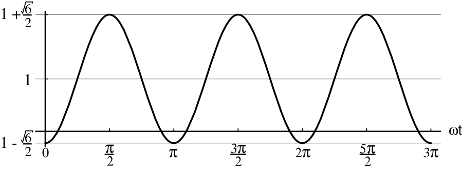
Figure 2.1: Time evolution of the energy density for the vacuum plus two particle state. Note that during every oscillation, the energy density dips below zero for a brief portion of the cycle. By manipulating the quantum state, it is possible to drive the energy density to increasingly negative values. Units on the vertical axis are in multiples of $\omega/2L^{3}$.

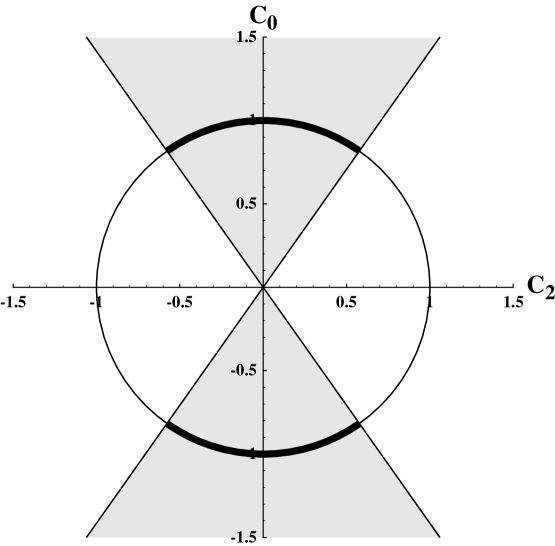
Figure 2.2: A plot showing the two conditions necessary to obtain negative energy densities for the vacuum plus two particle state. The normalization condition for the coefficients $c_{0}$ and $c_{2}$ is the unit circle. The necessary condition for negative energy $|c_{0}|>\sqrt{2}\,|c_{2}|$ is represented by the light gray region. The set of all possible states that meet both of these conditions is denoted by the bold curve at the top and bottom of the circle. The states with $|c_{0}|=1$ must be excluded because they correspond to the vacuum state, where the energy density is zero.

Actually, there are an infinite set of vacuum plus two particle states that give rise to negative energy densities. To show this, let us begin with a general superposition of an $n$ and an $n+2$ state,

$$|\psi\rangle=c_{n}|n_{\bf k}\rangle+c_{n+2}|n+2_{\bf k}\rangle,$$ (2.13)

where the normalization of the state is expressed by the condition

$$|c_{n}|^{2}+|c_{n+2}|^{2}=1.$$ (2.14)

There is an additional restriction that $|c_{n}|\neq 1$. This corresponds to a pure number eigenstate because the unit normalization would cause $c_{n+2}=0$.

For a superposition of the $n$ and $n+2$ particle states, the energy density is given by

$$\langle\psi|:T_{tt}:|\psi\rangle = {\omega\over L^{3}}\left(n+2|c_{n+2}|^{2}\right)-{\omega^{2}-m^{2}\over\omega L^{3}}\sqrt{(n+1)(n+2)}\times$$

$$\left[{\rm Re}(c_{n}^{*}c_{n+2})\cos 2({\bf k}\cdot{\bf x}-\omega t)-|{\rm Im}(c_{n}^{*}c_{n+2})|\sin 2({\bf k}\cdot{\bf x}-\omega t)\right].$$

In order to simplify our calculations, let us take $c_{n}$ and $c_{n+2}$ to be real. Then, in order to have negative energy densities, we must satisfy the condition

$$|c_{n}|>{\omega^{2}\over\omega^{2}-m^{2}}{1\over\sqrt{(n+1)(n+2)}}\left(2|c_{n+2}|+{n\over|c_{n+2}|}\right)\,.$$ (2.16)

In addition, we must satisfy the normalization condition (2.14), which for real coefficients is the equation for a unit circle in the ($c_{n},\,c_{n+2}$) plane.

For the massless ($m=0$) scalar field in the vacuum plus two particle state ($n=0$), the condition to obtain negative energy densities, Eq. (2.16), reduces to

$$|c_{0}|>\sqrt{2}\,|c_{2}|\,.$$ (2.17)

We can see from Figure 2.2 that any state, except $|c_{0}|=1$, that lies on the bold sections of the circle will satisfy both the above condition to obtain negative energy densities and the unit normalization condition. For real coefficients, $c_{n}$ and $c_{n+2}$, only the vacuum plus two particle state can generate negative energy densities. If we plot the condition to find negative energy densities, Eq. (2.16), for $c_{n}$ and $c_{n+2}$ real and $n\geq 1$, we find that the range of values that would allow negative energy densities is incompatible with the unit normalization condition.

2.1.2 Squeezed States

The squeezed states in quantum field theory can also produce negative energies. The squeezed states of light have been extensively investigated in the field of quantum optics and are realized experimentally. We will confine ourselves to the squeezed states of the quantized scalar field, although the treatment would be the same for the electromagnetic field.

We begin with the definition of two additional operators. The first, introduced by Glauber [51], is the displacement operator

$$D_{\bf k}(z)\equiv\exp\left(za_{\bf k}^{\dagger}-z^{*}a_{\bf k}\right)=e^{-|z|^{2}/2}e^{za_{\bf k}^{\dagger}}e^{-z^{*}a_{\bf k}},$$ (2.18)

which satisfies the commutation relations

$$\left[a_{\bf k^{\prime}},\,D_{\bf k}(z)\right] = a_{\bf k^{\prime}}+z\delta_{\bf kk^{\prime}},$$ (2.19)

$$\left[a_{\bf k^{\prime}}^{\dagger},\,D_{\bf k}(z)\right] = a_{\bf k^{\prime}}^{\dagger}+z^{*}\delta_{\bf kk^{\prime}}.$$ (2.20)

The second is the squeeze operator

$$S_{\bf k}(\zeta)\equiv\exp\left[{1\over 2}\zeta^{*}a_{\bf k}^{2}-{1\over 2}\zeta(a_{\bf k}^{\dagger})^{2}\right].$$ (2.21)

which satisfies the relations

$$S_{\bf k}^{\dagger}(\zeta)a_{\bf k}S_{\bf k}(\zeta) = a_{\bf k}\cosh r-a_{\bf k}^{\dagger}e^{i\delta}\sinh r,$$ (2.22)

$$S_{\bf k}^{\dagger}(\zeta)a_{\bf k}^{\dagger}S_{\bf k}(\zeta) = a_{\bf k}^{\dagger}\cosh r-a_{\bf k}e^{-i\delta}\sinh r.$$ (2.23)

The complex parameters $z$ and $\zeta$ may be written in terms of their magnitude and phases as

$$z=se^{i\gamma}\qquad\mbox{ and }\qquad\zeta=re^{i\delta}.$$ (2.24)

We can write a general squeezed state for a single mode as [52]

$$|\{z,\zeta\}_{\bf k}\rangle=D_{\bf k}(z)S_{\bf k}(\zeta)|0\rangle.$$ (2.25)

It has been shown that for a massless scalar field the expectation value of the energy density for the above squeezed state is given by [46]

$$\rho \equiv \langle\{z,\zeta\}_{\bf k}|:T_{tt}:|\{z,\zeta\}_{\bf k}\rangle,$$ (2.26)

$$= {\omega\over L^{3}}\left\{\sinh r\cosh r\cos(2\theta+\delta)+\sinh^{2}r+s^{2}\left[1-\cos 2(\theta+\gamma)\right]\right\},$$

where $\theta={\bf k}\cdot{\bf x}-\omega t$. When $\zeta=0$, the squeezed state reduces to a coherent state and the expectation value of the energy density is always positive definite. The coherent states are interpreted as the quantum states that describe classical field excitations. Thus, the production of only positive energy in coherent states is consistent with classical sources for gravity obeying the WEC.

A different case, known as the squeezed vacuum state, is defined when $z=0$. Such states result from quantum mechanical particle creation. An example is second harmonic generation in non-linear optical media. For the squeezed vacuum state, the energy density is given by

$$\langle\{0,\zeta\}_{\bf k}|:T_{tt}:|\{0,\zeta\}_{\bf k}\rangle={\omega\over L^{3}}\sinh r\left[\sinh r+\cosh r\cos(2\theta+\delta)\right].$$ (2.27)

The squeezed vacuum energy density will have the same negative energy density behavior as the vacuum plus two particle state above, with the energy density falling below zero once every cycle if the condition

$$\cosh r>\sinh r$$ (2.28)

is met. This happens to be true for every nonzero value of $r$, so the energy density becomes negative at some point in the cycle for a general squeezed vacuum state. In a more general state which is both squeezed and displaced, the energy density will become negative at some point in the cycle if $s\ll r$.

There are other interesting aspects of these states as well. When the quantum state is very close to a coherent state, we have seen that the energy density is usually not negative. In addition, fluctuations in the stress-tensor for these states are small compared to the expectation value of the stress-tensor in that state. On the other hand when the state is close to a squeezed vacuum state, there will almost always be some negative energy densities present, and the fluctuations in the expectation value of the stress-tensor start to become nearly as large as the expectation value itself. This seems to indicate that the semiclassical theory is beginning to break down [46].

2.2 The Quantized Fermion Field

In this section we will show that it is possible to generate negative energy densities using the fermion field. Therefore it does appear possible to use fermions to violate the weak energy condition. One example of a fermion state that produces negative energies has been demonstrated by Vollick [50] for a superposition of two single particle states traveling in different directions. The particular example that we will demonstrate has a particle content which is a superposition of the vacuum plus a particle-antiparticle pair. However the occurrence of negative energy densities for the above particle states can be a frame-dependent phenomenon. If the particle-antiparticle pair is traveling in the same direction, but with differing momenta, then it is possible for the energy density to become negative. However, in the center of mass frame of the particle-antiparticle pair, the local energy density always has a positive definite value.

The fermion field, denoted by $\psi(x)$, is the solution to the Dirac equation,

$$i\gamma^{\mu}\nabla_{\mu}\psi(x)-m\psi(x)=0,$$ (2.29)

where $m$ is the mass of the spin-$1\over 2$ particle, and the $\gamma^{\mu}$ are the the Dirac matrices in flat spacetime, which satisfy the anticommutation relations

$$\left\{\gamma^{\mu},\,\gamma^{\nu}\right\}=2g^{\mu\nu}.$$ (2.30)

The general solution of $\psi(x)$ can then be expanded in plane wave modes as

$$\psi(x)=\sum_{s}\int{d^{3}p\over(2\pi)^{3/2}}\sqrt{m\over E_{p}}\left[b(p,s)\,u(p,s)\,e^{-ip_{\mu}x^{\mu}}+d^{\dagger}(p,s)\,v(p,s)\,e^{ip_{\mu}x^{\mu}}\right]\,,$$ (2.31)

Here $b(p,s)$ and its hermitian conjugate $b^{\dagger}(p,s)$ are the annihilation and creation operators for the electron (fermion), respectively, while $d(p,s)$ and its hermitian conjugate $d^{\dagger}(p,s)$ are the respective annihilation and creation operators for the positron. All four operators anticommute except in the case

$$\left\{b(p,s),\,b^{\dagger}(p^{\prime},s^{\prime})\right\}=\delta_{ss^{\prime}}\delta^{3}(p-p^{\prime})=\left\{d(p,s),\,d^{\dagger}(p^{\prime},s^{\prime})\right\}.$$ (2.32)

The annihilation and creation operators for spin-${1\over 2}$ particles satisfy the anticommutation relations as opposed to the commutation relations for the scalar field because the fermions must obey the Pauli exclusion principle.

For the fermion field, the stress-tensor is given by [53]

$$T_{\mu\nu}={i\over 2}\left[\bar{\psi}\gamma_{(\mu}\nabla_{\nu)}\psi-\left(\nabla_{(\mu}\bar{\psi}\right)\gamma_{\nu)}\psi\right]\,.$$ (2.33)

Inserting the mode function expansion into the energy density, and then normal ordering by making use of the anticommutation relations, we find

$$T_{tt} = {1\over 2(2\pi)^{3}}\sum_{ss^{\prime}}\int d^{3}p\,d^{3}p^{\prime}{m\over\sqrt{E_{p}\,E_{p^{\prime}}}}(E_{p}+E_{p^{\prime}})\times$$ (2.34)

$$\;\times\left[b^{\dagger}(p^{\prime},s^{\prime})b(p,s)u^{\dagger}(p^{\prime},s^{\prime})u(p,s)e^{-i(p_{\mu}-p_{\mu}^{\prime})x^{\mu}}+d^{\dagger}(p,s)d(p^{\prime},s^{\prime})v^{\dagger}(p^{\prime},s^{\prime})v(p,s)e^{+i(p_{\mu}-p_{\mu}^{\prime})x^{\mu}}\right]$$

$$+{1\over 2(2\pi)^{3}}\sum_{ss^{\prime}}\int d^{3}p\,d^{3}p^{\prime}{m\over\sqrt{E_{p}\,E_{p^{\prime}}}}(E_{p}-E_{p^{\prime}})\times$$

$$\;\times\left[d(p^{\prime},s^{\prime})b(p,s)v^{\dagger}(p^{\prime},s^{\prime})u(p,s)e^{-i(p_{\mu}+p_{\mu}^{\prime})x^{\mu}}-b^{\dagger}(p,s)d^{\dagger}(p^{\prime},s^{\prime})u^{\dagger}(p^{\prime},s^{\prime})v(p,s)e^{+i(p_{\mu}+p_{\mu}^{\prime})x^{\mu}}\right]$$

$$-{1\over(2\pi)^{3}}\sum_{s}\int d^{3}p\,E_{p}\,.$$

Unlike the vacuum energy density for the scalar field, we see that the fermion field has an infinite negative energy density that must be removed by renormalization. Thus we again look at the fully normal ordered quantity,

$$:T_{tt}:=T_{tt}-\langle 0|T_{tt}|0\rangle.$$ (2.35)

While we are about to show that there are specific states for which the energy density can become negative, one should note that the Hamiltonian,

$$H=\int d^{3}x:T_{tt}:=\sum_{s}\int d^{3}p\,E_{p}\left[b^{\dagger}(p,s)b(p,s)+d^{\dagger}(p,s)d(p,s)\right]\,,$$ (2.36)

is always a positive definite quantity.

Now, we would like to show that the state

$$|\phi\rangle=c_{00}|0\rangle+c_{1\overline{1}}|k_{1}\,s_{1}\,;\overline{k_{2}\,s_{2}}\rangle\,,$$ (2.37)

admits negative energies for some values of $c_{00}$ and $c_{1\bar{1}}$. For purposes of clarity, we have defined the above states by

$$|k\,s\rangle = b^{\dagger}(k,s)|0\rangle\,,$$ (2.38)

$$|\overline{k\,s}\rangle = d^{\dagger}(k,s)|0\rangle\,,$$ (2.39)

$$|k_{1}\,s_{1}\,;\overline{k_{2}\,s_{2}}\rangle = d^{\dagger}(k_{2},s_{2})b^{\dagger}(k_{1},s_{1})|0\rangle=-|\overline{k_{2}\,s_{2}}\,;k_{1}\,s_{1}\rangle\,.$$ (2.40)

If we take the expectation value of the energy density with respect to this vacuum plus particle-antiparticle state, we find

$$\langle:T_{tt}:\rangle = {1\over(2\pi)^{3}}m|c_{1\bar{1}}|^{2}\left[u^{\dagger}(k_{1},s_{1})u(k_{1},s_{1})+v^{\dagger}(k_{2},s_{2})v(k_{2},s_{2})\right]$$

$$+ {m\over 2(2\pi)^{3}}{(E_{1}-E_{2})\over\sqrt{E_{1}E_{2}}}\left[c_{00}^{*}c_{1\bar{1}}\,v^{\dagger}(k_{2},s_{2})u(k_{1},s_{1})e^{-i(k_{1}^{\mu}+k_{2}^{\mu})x_{\mu}}+C.C.\right].$$

This expression is similar to the scalar field energy density for the vacuum plus two particle state. In order to have negative energy densities, we must find some combination of the mode functions and the coefficients $c_{00}$ and $c_{1\bar{1}}$ such that the amplitude of the interference term in the expression above is larger than the magnitude of the first term, which is the sum of the energy of the particle and antiparticle. In order to proceed any further, we must choose a specific form for the mode functions. This involves choosing a representation of the Dirac matrices. Let,

$$u(p,s)=\left[2m(E+m)\right]^{-1/2}\left(\matrix{(E+m)\,\phi(s)\cr(\mbox{\boldmath$\sigma$}\cdot{\bf p})\,\phi(s)\cr}\right)\,,$$ (2.42)

and

$$v(p,s)=\left[2m(E+m)\right]^{-1/2}\left(\matrix{(\mbox{\boldmath$\sigma$}\cdot{\bf p})\,\phi(s)\cr(E+m)\,\phi(s)\cr}\right)\,,$$ (2.43)

where ${\bf p}$ is the three momentum of the particle, $\sigma$ is the vector composed of the Pauli spin matrices, and $\phi(s)$ is a two-spinor. Using this basis, it is possible to show

$$u^{\dagger}(k,s)u(k,s^{\prime})={E_{k}\over m}\delta_{ss^{\prime}}=v^{\dagger}(k,s)v(k,s^{\prime}).$$ (2.44)

In addition, the interference term between the particle-antiparticle states is

$$v^{\dagger}(k_{2},s_{2})u(k_{1},s_{1})={{\phi^{\dagger}(s_{2})\mbox{\boldmath$\sigma$}\cdot\left[{\bf k}_{1}(E_{2}+m)+{\bf k}_{2}(E_{1}+m)\right]\phi(s_{1})}\over\sqrt{2m(E_{1}+m)(E_{2}+m)}}.$$ (2.45)

To evaluate the energy density explicitly at this point, let us take $s_{1}=s_{2}=+1$, therefore

$$\phi(s_{1})=\phi(s_{2})=\left(\matrix{1\cr 0\cr}\right).$$ (2.46)

For simplicity let the propagation vectors ${\bf k}_{1}$ and ${\bf k}_{2}$ both point in the $z$-direction, i.e.,

$$k_{1}^{\mu}=(E_{1},0,0,k_{1})\qquad\mbox{ and }\qquad k_{2}^{\mu}=(E_{2},0,0,k_{2})\,,$$ (2.47)

and let $c_{00}$ and $c_{1\bar{1}}$ be real. Then the energy density can be written as

$$\langle:T_{tt}:\rangle={c_{1\bar{1}}^{2}\over(2\pi)^{3}}(E_{1}+E_{2})+{c_{00}\,c_{1\bar{1}}\over 2(2\pi)^{2}}{(E_{1}-E_{2})\,\left[k_{1}(E_{2}+m)+k_{2}(E_{1}+m)\right]\over\sqrt{E_{1}E_{2}(E_{1}+m)(E_{2}+m)}}\,\cos(E_{1}+E_{2})t\,.$$ (2.48)

By an appropriate choice of the momenta and the coefficients $c_{00}$ and $c_{1\bar{1}}$ this can be made negative. This is most easily seen in the ultrarelativistic limit when $E\gg m$. The energy density is

$$\langle:T_{tt}:\rangle={E_{1}+E_{2}\over(2\pi)^{3}}c_{1\bar{1}}^{2}+{E_{1}-E_{2}\over(2\pi)^{3}}c_{00}c_{1\bar{1}}\cos(E_{1}+E_{2})t.$$ (2.49)

We then find that the energy density is negative, apart from the special case $c_{00}=1$, $c_{1\bar{1}}=0$ corresponding to the vacuum, when the condition

$$|c_{00}|\geq\left|{E_{1}+E_{2}\over E_{1}-E_{2}}c_{1\bar{1}}\right|$$ (2.50)

is met. Thus, an infinite number of states for negative energy densities could possibly exist.

It is interesting to note that in the center of mass frame of the particle-antiparticle pair, the local energy density in this state is a positive constant. This can easily be seen from Eq. (2.48), or more generally from Eq. (LABEL:eq:Gen_EDensity), when $E_{1}=E_{2}$ and $k_{1}=-k_{2}$. Thus, for a given particle content of the state, whether it is possible to detect negative energies is dependent upon the frame in which any measurement is to be carried out.

2.3 The Vacuum Energy

So far we have discussed only the cases where the particle content of the quantum state makes the energy density negative. These could be called coherence effects for the fields. As we have seen in the plane wave examples above, the negative energy densities are periodic in both space and time. For more general mode functions this need not be the case, and we could have various configurations of negative energy densities. However, it is also possible to generate negative energies without the presence of particles. The vacuum energy density of a spacetime can be positive or negative with respect to the Minkowski space vacuum after renormalization. Casimir originally proved this in 1948 for the electromagnetic field between two perfectly conducting planar plates [9]. Here the energy density between the two plates is negative. Similar effects can be shown in gravitational physics. For example, the vacuum energy is non-zero for the scalar field in Einstein’s universe and can be positive or negative, depending on our choice of either minimal or conformal coupling for the interaction between gravity and the scalar field in the wave equation,

$$g^{\mu\nu}\nabla_{\mu}\nabla_{\nu}\,\phi(x)-\left(m^{2}+\xi R(x)\right)\,\phi(x)=0.$$ (2.51)

Minimal coupling is $\xi=0$, while conformal coupling is given by

$$\xi(n)={1\over 4}{(n-2)\over(n-1)}\,,$$ (2.52)

where $n$ is the dimensionality of the spacetime. In four dimensions $\xi=1/6$, while in two dimensions, minimal and conformal coupling are the same. The vacuum energy density for a massless scalar field in the four-dimensional static Einstein universe [15, 35] is

$$\rho_{vacuum}=-{0.411505\over 4\pi^{2}a^{4}}$$ (2.53)

for minimal coupling. Meanwhile, for conformal coupling the vacuum energy density is [13, 14]

$$\rho_{vacuum}=+{1\over 480\pi^{2}a^{4}}.$$ (2.54)

Here, $a$ is the scale factor of the closed universe. We will discuss more fully the derivation of the vacuum energy for minimal coupling in Einstein’s universe in Section 4.3.3, when we renormalize the quantum inequality in Einstein’s universe. At this point we would like to discuss a slightly simpler example, the vacuum energy near a planar conductor in both two dimensions and four dimensions.

2.3.1 Renormalization

We begin with a massless scalar field in Minkowski spacetime with no boundaries. The positive frequency mode function solutions for the scalar wave equation are

$$f_{\bf k}({\bf x},t)=(4\pi\omega)^{-1/2}\,e^{i({\bf k\cdot x}-\omega t)}\,,$$ (2.55)

where $-\infty<{\bf k}<+\infty$ is the mode label, and $\omega=|{\bf k}|$ is the energy. In the case of arbitrary coupling, the stress-tensor is

$$T_{\mu\nu}=(1-2\xi)\phi_{,\mu}\phi_{,\nu}+(2\xi-1/2)\eta_{\mu\nu}\eta^{\rho\sigma}\phi_{,\rho}\phi_{,\sigma}-2\xi\phi_{,\mu\nu}\phi\,.$$ (2.56)

We could proceed by placing the mode function expansion for the field $\phi({\bf x},t)$ into the expression for the stress-tensor above and then taking the expectation value as we did in the preceding sections. We would find the infinite positive energy density as we have previously and then subtract it away to find the renormalized energy density. There is an alternative method using the Wightman function, defined as

$$D^{+}(x,x^{\prime})=\langle 0|\phi(x)\phi(x^{\prime})|0\rangle.$$ (2.57)

The expectation value of the stress-tensor above in the vacuum state can be written equivalently as

$$\langle 0|T_{\mu\nu}|0\rangle=\lim_{x^{\prime}\rightarrow x}\left[(1-2\xi)\partial_{\mu}\partial^{\prime}_{\nu}+(2\xi-1/2)g_{\mu\nu}g^{\rho\sigma}\partial_{\rho}\partial^{\prime}_{\sigma}-2\xi\partial_{\mu}\partial_{\nu}\right]D^{+}(x,x^{\prime}),$$ (2.58)

where $\partial_{\mu}$ is the ordinary derivative in the unprimed coordinates and $\partial^{\prime}_{\nu}$ in the primed coordinates. The process of renormalization involves removing any infinities by subtracting away the equivalent infinity in the Minkowski vacuum. This can be accomplished by renormalizing the Wightman function before we act on it with the derivative operator to find the expectation value of the stress-tensor. The renormalized Wightman function is defined as

$$D^{+}_{Ren.}(x,x^{\prime})=D^{+}(x,x^{\prime})-D^{+}_{Minkowski}(x,x^{\prime}).$$ (2.59)

We see that the renormalized vacuum energy in Minkowski space is then set to zero. A similar formalism can be carried out for curved spacetimes as well. To find the renormalized Wightman function, we would first find the regular Wightman function. Then we subtract away the Wightman function that would be found by taking its limit when the spacetime becomes flat. However, in curved spacetimes, this does not remove all of the infinities in the stress-tensor. There may be logarithmic and/or curvature-dependent divergences which must also be removed.

2.3.2 Vacuum Energies for Mirrors

Let us start by considering the case of a two-dimensional flat spacetime in which we place a perfectly reflecting mirror at the origin. In two-dimensional Minkowski spacetime, the Wightman function is found to be

$$D^{+}_{Minkowksi}(x,x^{\prime})=-{1\over 4\pi}\ln\left[(t-t^{\prime})^{2}-(z-z^{\prime})^{2}\right].$$ (2.60)

However, we do not expect this to be the Wightman function when the mirror is present. That is because the mode functions will be altered in such a way that they vanish on the surface of the mirror. Because the spacetime is still flat, just with a perfectly reflecting boundary, the new Wightman function can be found by the method of images, with a source at spacetime point to be $x^{\prime}$, and the observation point at $x$. The Wightman function with the mirror present is now composed of two terms,

$$D^{+}(x,x^{\prime})=-{1\over 4\pi}\ln\left[(t-t^{\prime})^{2}-(z-z^{\prime})^{2}\right]+{1\over 4\pi}\ln\left[(t-t^{\prime})^{2}-(z+z^{\prime})^{2}\right].$$ (2.61)

To renormalize the Wightman function, we now subtract away the Minkowski Wightman function yielding

$$D^{+}_{Ren.}(x,x^{\prime})={1\over 4\pi}\ln\left[(t-t^{\prime})^{2}-(z+z^{\prime})^{2}\right].$$ (2.62)

The vacuum energy density in this spacetime is then

$$\langle 0|T_{tt}|0\rangle_{Ren.}=\lim_{x^{\prime}\rightarrow x}\left[{1\over 2}\partial_{t}\partial_{t^{\prime}}+({1\over 2}-2\xi)\partial_{z}\partial_{z^{\prime}}-2\xi\partial_{t}\partial_{t}\right]{1\over 4\pi}\ln\left[(t-t^{\prime})^{2}-(z+z^{\prime})^{2}\right]={\xi\over 2\pi z^{2}}.$$ (2.63)

Similar calculations can be carried out for the other components of the stress-tensor to find

$$\langle 0|T_{\mu\nu}|0\rangle_{Ren.}={\xi\over 2\pi z^{2}}\left[\begin{array}[]{cc}1&0\\ 0&0\\ \end{array}\right].$$ (2.64)

We see that the vacuum energy density is non-zero for any value of $\xi\neq 0$. In addition, the energy density diverges as one approaches the mirror. The actual sign of the energy density depends on the sign of the coupling constant, so we can have infinite positive as well as negative energy densities. However, at large distances away from the mirror the vacuum energy density rapidly goes to zero.

Similar results can be found for a planar perfectly reflecting mirror in four dimensions. With the mirror located in the $xy$-plane at $z=0$ the renormalized Green’s function for a massless scalar field is

$$D^{+}_{Ren.}(x,x^{\prime})=-{1\over 4\pi^{2}}\left[(x-x^{\prime})^{2}+(y-y^{\prime})^{2}+(z+z^{\prime})^{2}-(t-t^{\prime})^{2}\right]^{-1}.$$ (2.65)

Using Eq. (2.58) we find

$$\langle 0|T_{\mu\nu}|0\rangle_{Ren.}={1-6\xi\over 16\pi^{2}z^{4}}\left[\begin{array}[]{rrrr}-1&0&0&0\\ 0&1&0&0\\ 0&0&1&0\\ 0&0&0&0\\ \end{array}\right].$$ (2.66)

As was the case with the two-dimensional plate, the four-dimensional vacuum energy still diverges as one approaches the mirror surface. In addition, there are different values of the coupling constant $\xi$ that cause different effects on the stress-tensor. For the coupling constant less than $1/6$, the energy density is everywhere negative and the transverse pressures are positive. In addition, both are divergent on the mirror’s surface. This includes the often used case of minimal coupling, $\xi=0$. When the coupling constant is equal to $1/6$, the conformally coupled case, the energy density and transverse pressures vanish. Finally, when the coupling constant becomes greater than $1/6$, the energy density becomes positive and is still divergent at the mirror. However, the transverse pressures now become negative. These are summarized in Table 2.1. One should note that for all values of the coupling constant, the component of the pressure that is perpendicular to the surface to the mirror, the $z$-direction, is always zero.

Value of Coupling Constant	Energy Density	Transverse Pressure
$\xi$	$\langle T_{tt}\rangle$	$\langle T_{xx}\rangle=\langle T_{yy}\rangle$
$\xi<{1/6}$	$<0$	$>0$
$\xi={1/6}$	$0$	$0$
$\xi>{1/6}$	$>0$	$<0$

Table 2.1: Vacuum energy density and pressures for a perfectly reflecting mirror in four dimensions as a function of the coupling parameter $\xi$.

2.3.3 The Casimir Force

Let us consider two perfectly conducting planar plates, parallel to each other and separated by a distance L along the $z$-axis. Between the two conducting plates, the stress-tensor of the scalar field for conformal coupling is given by [54, 55]

$$\langle 0|T_{\mu\nu}|0\rangle_{Conf.}={\pi^{2}\over 1440L^{4}}\left[\begin{array}[]{rrrr}-1&0&0&0\\ 0&1&0&0\\ 0&0&1&0\\ 0&0&0&-3\\ \end{array}\right].$$ (2.67)

In the case of minimal coupling it is given by

$$\langle 0|T_{\mu\nu}|0\rangle_{Min.}=\langle 0|T_{\mu\nu}|0\rangle_{Conf.}+{\pi^{2}\over 48L^{4}}{3-2\sin^{2}(\pi z/L)\over\sin^{4}(\pi z/L)}\left[\begin{array}[]{rrrr}-1&0&0&0\\ 0&1&0&0\\ 0&0&1&0\\ 0&0&0&0\\ \end{array}\right].$$ (2.68)

In the region outside of the plates, the stress-tensor is given by Eq. (2.66). The net force, $F$, per unit area, $A$, acting on the plates is then given by the difference of the $T_{zz}$ component of the stress-tensor on opposite sides of the plate. For both minimal and conformal coupling, there is an attractive force between the two plates with a magnitude

$$|F(L)/A|={\pi^{2}\over 480\,L^{4}}.$$ (2.69)

Similarly, for the quantized electromagnetic field between two conducting plates, the attractive force between the plates is

$$|F(L)/A|={\pi^{2}\over 240\,L^{4}}.$$ (2.70)

The factor of two difference comes about because the electromagnetic field has two polarization states. Lamoreaux has confirmed the existence of this force experimentally [10]. This was done by measuring the force of attraction between a planar disk and a spherical lens, both of which were plated in gold. The Casimir force is known to be independent of the molecular structure of the conductors, provided the material is a near perfect conductor, but sensitive to the actual geometry of the plates. Attempts to measure the force between two parallel plates were unsuccessful because of the difficulty in trying to maintain parallelism to the required accuracy of $10^{-5}$ radians. For the plate and sphere, there is no issue of parallelism, and the system is described by the separation of the points of closest approach. However the Casimir force for this geometry is not given by (2.70), but has the form

$$F(a)={2\pi aR\over 3}\left({\pi^{2}\over 240a^{4}}\right),$$ (2.71)

where $R$ is the radius of curvature of the spherical surface and $a$ is the distance of closest approach. In addition, the force is independent of the plate area. Lamoreaux finds that the experimentally measured force agrees with the predicted theory at the level of 5%. With direct confirmation of the Casimir force, we must admit that the vacuum effects in the stress-tensor are not merely a mathematical curiosity, but have direct physical consequences. In general relativity this is extremely important because the vacuum stress-tensor can act as a source of gravity.

2.3.4 Vacuum Stress-Tensor for Two-Dimensional Stars

In all of the examples of the preceding section for vacuum energy densities, we studied how the effects of boundary conditions on the scalar field can induce the vacuum to take on a non-zero value in flat spacetime. We saw that the energy density near a perfectly reflecting mirror becomes divergent on the surface to the plate. It is interesting to note that non-zero vacuum energies can also be found in gravitational physics. In some sense, the non-zero value of the stress-tensor is more important in gravitational physics because it can serve as a source in Einstein’s equation. Thus the vacuum energy can have non-trivial effects on the evolution of the spacetime. The most well known, and well studied example of this is the evaporation of black holes, originally demonstrated by Hawking [56]. In this section we will study a slightly different problem, the vacuum energy for a massless scalar field on the background spacetime of a constant density star.

We begin with the metric of a static spherically symmetric star composed of a classical incompressible constant density fluid. The metric for this type of star is well known [57],

$$ds^{2}=-B(r)dt^{2}+A(r)dr^{2}+r^{2}d\Omega^{2},$$ (2.72)

where $d\Omega^{2}$ is the length element on a unit sphere, and the functions $A(r)$ and $B(r)$ are defined by

$$A(r)=\left\{\begin{array}[]{ll}\left[1-{2Mr^{2}/R^{3}}\right]^{-1}&\mbox{ for }r\leq R,\\ \left[1-{2M/r}\right]^{-1}&\mbox{ for }r>R,\end{array}\right.$$ (2.73)

and

$$B(r)=\left\{\begin{array}[]{ll}{1\over 4}\left[3\left(1-{2M/R}\right)^{1/2}-\left(1-{2Mr^{2}/R^{3}}\right)^{1/2}\right]^{2}&\mbox{ for }r\leq R,\\ \left[1-{2M/r}\right]&\mbox{ for }r>R.\end{array}\right.$$ (2.74)

Here $M$ is the mass of the star and $R$ its radius. This metric has one constraint: The mass and radius must satisfy

$$R>{9\over 8}\,(2M)\,.$$ (2.75)

Otherwise the pressure at the core of the star will become singular. This radius is just slightly larger than the Schwarzschild radius of a black hole of the same mass. When a star becomes sufficiently compact and its radius approaches the above limit, then the gravitational back-reaction should start to have a significant effect on the spacetime. For the rest of our calculations we will presume that condition (2.75) is satisfied. It would be a rather arduous task to find the vacuum stress-tensor for the four-dimensional spacetime. However, we can make significant progress for the two-dimensional equivalent with the metric

$$ds^{2}=-B(r)dt^{2}+A(r)dr^{2}\,.$$ (2.76)

This metric can be recast into its null form

$$ds^{2}=-B(r)\,dU\,dV\,,$$ (2.77)

where the null coordinates are defined by

$$U=t-r^{*}\qquad\mbox{ and }\qquad V=t+r^{*},$$ (2.78)

with $r^{*}$ given by

$$r^{*}=\int\sqrt{A(r)\over B(r)}\,dr.$$ (2.79)

It is clear from the form of the metric (2.77) that this spacetime, like all two-dimensional spacetimes, is conformally flat. Thus, we can apply the method of finding the vacuum stress-tensor in two-dimensional spacetimes, [58] and Section 8.2 of [53]. The stress-tensor components of the vacuum, obtained when positive frequency modes are defined by the timelike Killing vector, in the $(U,V)$ coordinates are

$$\langle 0|T_{UU}|0\rangle=\langle 0|T_{VV}|0\rangle={1\over 192\pi}\left[2BB^{\prime\prime}-(B^{\prime})^{2}\right]$$ (2.80)

and

$$\langle 0|T_{UV}|0\rangle={1\over 96\pi}BB^{\prime\prime}\,,$$ (2.81)

where the prime denotes the derivative with respect to $r$. By a coordinate transformation, we can calculate the components of the stress-tensor in the original $(r,t)$ coordinates,

$$\langle 0|T_{\mu\nu}(t,r)|0\rangle={1\over 24\pi}\left[\begin{array}[]{cc}B(r)B^{\prime\prime}(r)-{1\over 4}B^{\prime}(r)^{2}&0\\ 0&-{1\over 4}A(r)B^{\prime}(r)^{2}/B(r)\end{array}\right].$$ (2.82)

We can now directly calculate the value of the vacuum stress-tensor both outside and inside the star. In the exterior region of the star, the stress-tensor is given by

$$\langle 0|T_{\mu\nu}|0\rangle_{exterior}={1\over 24\pi}\left[\begin{array}[]{cc}(7M^{2}/r^{4}-4M/r^{3})&0\\[8.0pt] 0&-(M^{2}/r^{4})(1-2M/r)^{-2}\end{array}\right].$$ (2.83)

This is the well known result for the Boulware vacuum of a black hole [59]. We can see that for the stationary observer at a fixed radius outside of the star that the energy density is

$$\rho_{exterior}(r)={(7M^{2}/r^{4}-4M/r^{3})\over 24\pi(1-2M/r)}.$$ (2.84)

For the case of the star, the exterior region does not reach all the way to the Schwarzschild radius, so there is no divergence as there was for a black hole. However, the energy density for an observer fixed at some constant distance away from the star is still negative.

The situation is somewhat different in the interior of the star. The stress-tensor components are given by

$$\langle 0|T_{\mu\nu}|0\rangle_{interior}={A(r)\over 24\pi}\left[\begin{array}[]{cc}B(r){M\over R^{3}}\left[3\sqrt{A(r)\left(1-{2M\over R}\right)}-1+{Mr^{2}\over R^{3}}\right]&0\\[8.0pt] 0&-A(r){M^{2}r^{2}\over R^{6}}\end{array}\right].$$ (2.85)

The vacuum energy density for the interior of the star as seen by a stationary observer is

$$\rho_{interior}(r)={1\over 24\pi}\left(1-{2Mr^{2}\over R^{3}}\right)^{-1}\left({M\over R^{3}}\right)\left[3\sqrt{A(r)\left(1-{2M\over R}\right)}-1+{Mr^{2}\over R^{3}}\right].$$ (2.86)

It is not immediately obvious, but the energy density in the interior is everywhere positive, and grows in magnitude as we move outward from the center of the star, as plotted in Figure 2.3. In contrast, the vacuum energy outside the star is negative and identical to that of the black hole in the Boulware vacuum state. The discontinuity in the vacuum energy is an effect of the star having a very abrupt change in the mass density when crossing the surface of the star. We presume that if the star makes a continuous transition from the constant density core to the vacuum exterior then the vacuum energy would smoothly pass through zero.

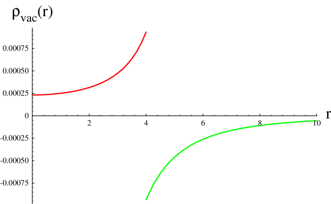
Figure 2.3: The vacuum energy density induced inside and outside a star. Here we have taken the star to be composed of some form of classical matter that has a constant density throughout. The vacuum energy is then calculated for a scalar field which does not interact with the matter, except that it is subject to the spacetime curvature. Units have been normalized such that the mass of the star is unity. The radius of the star is 4 units.

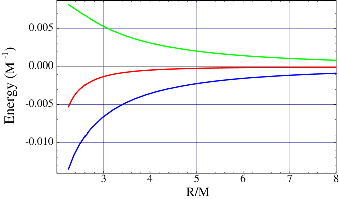
Figure 2.4: The total integrated vacuum energy density induced inside and outside a star as a function of the radius. The top line is the contribution from the positive energy in the interior of the star. The lower line is the contribution from the exterior Boulware vacuum energy. The middle line is the total over all space. The energy is in units of inverse mass.

The total vacuum energy of this spacetime can be found by integrating the local energy density over all space. The total positive vacuum energy contained inside the star is

$$E_{inside}=2\int_{0}^{R}\rho(r)\,dr\,=\,{1\over 48\pi R^{2}}\left(10M-\sqrt{2MR}\,\tanh^{-1}\sqrt{2M\over R}\right).$$ (2.87)

The contribution outside the star gives a total finite negative energy

$$E_{outside}=2\int_{R}^{\infty}\rho(r)\,dr\,=\,-{1\over 96\pi}\left[{14M\over R^{2}}-{2\over R}-{1\over M}\ln\left(1-{2M\over R}\right)\right].$$ (2.88)

The total energy due to the vacuum is the sum

$$E_{Total}=E_{inside}+E_{outside}\,.$$ (2.89)

This is always finite and negative, as shown in Figure 2.4 along with the individual contributions from the interior and exterior of the star. For very diffuse stars, $R\gg 2M$, the total positive interior vacuum energy very nearly compensates for the negative energy outside the star. In this limit the leading contributions to the total energy go as

$$E_{Total}\sim-{M^{2}\over 18\pi R^{3}}-{3M^{3}\over 40\pi R^{4}}-O(R^{-5})-\cdots.$$ (2.90)

In the other regime, when the star becomes very compact, the Boulware vacuum begins to dominate and in the limit $R\rightarrow 9M/4$, the energy density goes to its finite minimum value $E_{min}=-5.306574\times 10^{-3}\,M^{-1}$. This residual energy can be considered a mass renormalization of the star due to the vacuum polarization,

$$M=M_{bare}+\delta M=M_{bare}-{5.306574\times 10^{-3}\over M}M_{Planck}^{2}.$$ (2.91)

Unless the mass of the star is very close to the Planck mass, $M_{Planck}$, this correction to the effective mass of the star is extremely small, accounting for at most half a percent of the star’s mass.

Chapter 3 Derivation of the Quantum Inequalities

3.1 General Theory for Quantized Scalar Fields

We begin by considering the semiclassical theory of gravity, where the classical Einstein tensor on the left-hand side of Eq. (3.1) is equal to the expectation value of the stress-energy tensor (stress-tensor) of a quantized field on the right-hand side,

$$G_{\mu\nu}=8\pi\;\langle T_{\mu\nu}\rangle\;.$$ (3.1)

Here we are using Planck units, in which $\hbar=c=G=1$. We will take the stress-tensor to be that of the massive, minimally coupled scalar field, $\phi(x)$, given by

$$T_{\mu\nu}=\phi_{;\mu}\phi_{;\nu}-{1\over 2}g_{\mu\nu}\phi^{;\rho}\phi_{;\rho}+{1\over 2}m^{2}g_{\mu\nu}\phi^{2}\;,$$ (3.2)

where $\phi_{;\alpha}$ denotes the covariant derivative of $\phi$ on the classical background metric and $m$ is the mass of the field. We shall develop quantum inequalities in globally static spacetimes, those in which $\partial_{t}$ is a timelike Killing vector. Such a metric can be written in the form

$${ds}^{2}=-|g_{tt}({\bf x})|{dt}^{2}+g_{ij}({\bf x})dx^{i}dx^{j}\;,$$ (3.3)

where the function $g_{tt}({\bf x})$ is related to the red or blue shift dependent only on the observer’s position in space, and $g_{ij}({\bf x})$ is the metric of the spacelike hypersurfaces that are orthogonal to the Killing vector in the time direction. With this metric, the wave equation

$$\mathord{\hbox{\Bxfnt\char 116\relax}\hbox to0.0pt{\hss\Bxfnt\char 117\relax}}\phi-m^{2}\phi={1\over\sqrt{|g|}}\left(\partial_{\alpha}\sqrt{|g|}g^{\alpha\beta}\partial_{\beta}\phi\right)-m^{2}\phi=0$$ (3.4)

becomes

$$-{1\over|g_{tt}|}\partial_{t}^{2}\phi+\nabla^{i}\nabla_{i}\phi-m^{2}\phi=0,$$ (3.5)

where $g={\rm det}(g_{\mu\nu})$. The timelike Killing vector allows us to use a separation of variables to find solutions of the wave equation. The positive frequency mode function solutions can be written as

$$f_{\lambda}({\bf x},t)=\,U_{\lambda}({\bf x})\,e^{-i\omega t}.$$ (3.6)

The label $\lambda$ represents the set of quantum numbers necessary to specify the mode. Additionally, the mode functions should have unit Klein-Gordon norm

$$\left(f_{\lambda},f_{\lambda^{\prime}}\right)=\delta_{\lambda\lambda^{\prime}}.$$ (3.7)

A general solution of the scalar field $\phi$ can then be expanded in terms of creation and annihilation operators as

$$\phi=\sum_{\lambda}{\bigl{(}a_{\lambda}f_{\lambda}+a^{\dagger}_{\lambda}f^{\ast}_{\lambda}\bigr{)}},$$ (3.8)

when quantization is carried out over a finite box or universe. If the spacetime is itself infinite, then we replace the summation by an integral over all of the possible modes. The creation and annihilation operators satisfy the usual commutation relations [53].

In principle, quantum inequalities can be found for any geodesic observer [32]. In many curved spacetimes, static observers often view the universe as having certain symmetries. By making use of these symmetries, we can often simplify calculations or equations. To observers moving along timelike geodesics the symmetries of the rest observers may not be “observable.” In the most general sense, the mode functions of the wave equation in a moving frame may become quite complicated. Thus, we will concern ourselves only with static observers, whose four-velocity, $u^{\mu}=({1\over\sqrt{|g_{tt}|}},{\bf 0})$, is in the direction of the timelike Killing vector. The energy density that such an observer measures is given by

$$\rho=T_{\mu\nu}u^{\mu}u^{\nu}={1\over|g_{tt}|}T_{tt}={1\over 2}\left[{1\over|g_{tt}|}(\partial_{t}\phi)^{2}+\nabla^{j}\phi\nabla_{j}\phi+m^{2}\phi^{2}\right]\,.$$ (3.9)

Upon substitution of the mode function expansion into Eq. (3.9), we find

$$\rho = {\rm Re}\sum_{\lambda\lambda^{\prime}}\left\{{{\omega\omega^{\prime}}\over|g_{tt}|}\left[U_{\lambda}^{*}U_{\lambda^{\prime}}e^{+i(\omega-\omega^{\prime})t}a_{\lambda}^{\dagger}a_{\lambda^{\prime}}-U_{\lambda}U_{\lambda^{\prime}}e^{-i(\omega+\omega^{\prime})t}a_{\lambda}a_{\lambda^{\prime}}\right]\right.$$ (3.10)

$$\qquad+\left[\nabla^{j}U_{\lambda}^{*}\nabla_{j}U_{\lambda^{\prime}}e^{+i(\omega-\omega^{\prime})t}a_{\lambda}^{\dagger}a_{\lambda^{\prime}}+\nabla^{j}U_{\lambda}\nabla_{j}U_{\lambda^{\prime}}e^{-i(\omega+\omega^{\prime})t}a_{\lambda}a_{\lambda^{\prime}}\right]$$

$$\qquad+m^{2}\left.\left[U_{\lambda}^{*}U_{\lambda^{\prime}}e^{+i(\omega-\omega^{\prime})t}a_{\lambda}^{\dagger}a_{\lambda^{\prime}}+U_{\lambda}U_{\lambda^{\prime}}e^{-i(\omega+\omega^{\prime})t}a_{\lambda}a_{\lambda^{\prime}}\right]\right\}$$

$$+{1\over 2}\sum_{\lambda}\left({\omega^{2}\over|g_{tt}|}U_{\lambda}^{*}U_{\lambda}+\nabla^{j}U_{\lambda}^{*}\nabla_{j}U_{\lambda}+m^{2}U_{\lambda}^{*}U_{\lambda}\right)\,.$$

The last term is the expectation value in the vacuum state, defined by $a_{\lambda}|0\rangle=0$ for all $\lambda$, and is formally divergent. The vacuum energy density may be defined by a suitable regularization and renormalization procedure, discussed in more detail later in Sections 4.2.3 and 4.3.2. In general, however, it is not uniquely defined. This ambiguity may be side-stepped by concentrating attention upon the difference between the energy density in an arbitrary state and that in the vacuum state, as was done by Ford and Roman [32]. We will therefore concern ourselves primarily with the difference defined by

$$:\rho:\;=\rho-\langle 0|\rho|0\rangle,$$ (3.11)

where $|0\rangle$ represents the Fock vacuum state defined by the global timelike Killing vector.

The renormalized energy density as defined above is valid along the entire worldline of the the observer. However, let us suppose that the energy density is only sampled along some finite interval of the geodesic. This may be accomplished by means of a weighting function which has a characteristic time $t_{0}$. The Lorentzian function,

$$f(t)={t_{0}\over\pi}\,{1\over{t^{2}+t_{0}^{2}}}\,,$$ (3.12)

is a good choice. The integral over all time of $f(t)$ yields unity and the width of the Lorentzian is characterized by $t_{0}$. Using such a weighting function, we find that the averaged energy difference is given by

$$\Delta\hat{\rho} \equiv {t_{0}\over\pi}\int_{-\infty}^{\infty}{{\langle:T_{tt}/|g_{tt}|:\rangle dt}\over{t^{2}+t_{0}^{2}}}$$ (3.13)

$$= {\rm Re}\sum_{\lambda\lambda^{\prime}}\left\{{{\omega\omega^{\prime}}\over|g_{tt}|}\left[U_{\lambda}^{*}U_{\lambda^{\prime}}e^{-|\omega-\omega^{\prime}|t_{0}}\langle a_{\lambda}^{\dagger}a_{\lambda^{\prime}}\rangle-U_{\lambda}U_{\lambda^{\prime}}e^{-(\omega+\omega^{\prime})t_{0}}\langle a_{\lambda}a_{\lambda^{\prime}}\rangle\right]\right.$$

$$\qquad+\left[\nabla^{j}U_{\lambda}^{*}\nabla_{j}U_{\lambda^{\prime}}e^{-|\omega-\omega^{\prime}|t_{0}}\langle a_{\lambda}^{\dagger}a_{\lambda^{\prime}}\rangle+\nabla^{j}U_{\lambda}\nabla_{j}U_{\lambda^{\prime}}e^{-(\omega+\omega^{\prime})t_{0}}\langle a_{\lambda}a_{\lambda^{\prime}}\rangle\right]$$

$$\qquad+\,m^{2}\left.\left[U_{\lambda}^{*}U_{\lambda^{\prime}}e^{-|\omega-\omega^{\prime}|t_{0}}\langle a_{\lambda}^{\dagger}a_{\lambda^{\prime}}\rangle+U_{\lambda}U_{\lambda^{\prime}}e^{-(\omega+\omega^{\prime})t_{0}}\langle a_{\lambda}a_{\lambda^{\prime}}\rangle\right]\right\}\,.$$

We are seeking a lower bound on this quantity. It has been shown [47, 48] that

$${\rm Re}\sum_{\lambda\lambda^{\prime}}f(\lambda)^{*}f(\lambda^{\prime})e^{-|\omega-\omega^{\prime}|t_{0}}\langle a_{\lambda}^{\dagger}a_{\lambda^{\prime}}\rangle\geq{\rm Re}\sum_{\lambda\lambda^{\prime}}f(\lambda)^{*}f(\lambda^{\prime})e^{-(\omega+\omega^{\prime})t_{0}}\langle a_{\lambda}^{\dagger}a_{\lambda^{\prime}}\rangle.$$ (3.14)

Upon substitution of this into Eq. (3.13) we have

$$\Delta\hat{\rho} \geq {\rm Re}\sum_{\lambda\lambda^{\prime}}\left\{{{\omega\omega^{\prime}}\over|g_{tt}|}\left[U_{\lambda}^{*}U_{\lambda^{\prime}}\langle a_{\lambda}^{\dagger}a_{\lambda^{\prime}}\rangle-U_{\lambda}U_{\lambda^{\prime}}\langle a_{\lambda}a_{\lambda^{\prime}}\rangle\right]\right.$$ (3.15)

$$\qquad+\left[\nabla^{j}U_{\lambda}^{*}\nabla_{j}U_{\lambda^{\prime}}\langle a_{\lambda}^{\dagger}a_{\lambda^{\prime}}\rangle+\nabla^{j}U_{\lambda}\nabla_{j}U_{\lambda^{\prime}}\langle a_{\lambda}a_{\lambda^{\prime}}\rangle\right]$$

$$\qquad+m^{2}\left.\left[U_{\lambda}^{*}U_{\lambda^{\prime}}\langle a_{\lambda}^{\dagger}a_{\lambda^{\prime}}\rangle+U_{\lambda}U_{\lambda^{\prime}}\langle a_{\lambda}a_{\lambda^{\prime}}\rangle\right]\right\}e^{-(\omega+\omega^{\prime})t_{0}}\,.$$

We may now apply the inequalities proven in Appendix A. For the first and third term of Eq. (3.15), apply Eq. (A.7) with $h_{\lambda}=\omega/\sqrt{|g_{tt}|}\,U_{\lambda}{\rm e}^{-\omega t_{0}}$ and $h_{\lambda}=m\,U_{\lambda}{\rm e}^{-\omega t_{0}}$, respectively. For the second term of Eq. (3.15), apply Eq. (A.1) with $A_{ij}=g_{ij}$ and $h_{\lambda}^{i}=\nabla^{i}U_{\lambda}{\rm e}^{-\omega t_{0}}$. The result is

$$\Delta\hat{\rho}\geq-{1\over 2}\sum_{\lambda}\left({\omega_{\lambda}^{2}\over|g_{tt}|}U_{\lambda}^{*}U_{\lambda}+\nabla^{j}U_{\lambda}^{*}\,\nabla_{j}U_{\lambda}+m^{2}U_{\lambda}^{*}U_{\lambda}\right)e^{-2\omega_{\lambda}t_{0}}.$$ (3.16)

This inequality may be rewritten using the Helmholtz equation satisfied by the spatial mode functions:

$$\nabla^{j}\nabla_{j}U_{\lambda}+(\omega^{2}/|g_{tt}|-m^{2})U_{\lambda}=0\,,$$ (3.17)

to obtain

$$\Delta\hat{\rho}\geq-\sum_{\lambda}\left({\omega_{\lambda}^{2}\over|g_{tt}|}+{1\over 4}\nabla^{j}\nabla_{j}\right)|U_{\lambda}|^{2}{\rm e}^{-2\omega_{\lambda}t_{0}}\,.$$ (3.18)

This can be rewritten as

$$\Delta\hat{\rho}\geq-{1\over 4}\left({\partial_{t_{0}}^{2}\over|g_{tt}|}+\nabla^{j}\nabla_{j}\right)\sum_{\lambda}|U_{\lambda}({\bf x})|^{2}{\rm e}^{-2\omega_{\lambda}t_{0}}\,.$$ (3.19)

There is a more compact notation in which Eq. (3.19) may be expressed. If we take the original metric, Eq. (3.3), and Euclideanize the time by allowing $t\rightarrow it_{0}$, then the Euclidean box operator is defined by

$$\mathord{\hbox{\Bxfnt\char 116\relax}\hbox to0.0pt{\hss\Bxfnt\char 117\relax}}_{E}\equiv{\partial_{t_{0}}^{2}\over|g_{tt}|}+\nabla^{j}\nabla_{j}\,.$$ (3.20)

The analytic continuation of the Feynman Green’s Function to imaginary time yields the Euclidean two-point function. The two are related by

$$G_{E}({\bf x},t;{\bf x}^{\prime},t^{\prime})=iG_{F}({\bf x},-it;{\bf x}^{\prime},-it^{\prime}).$$ (3.21)

In terms of the mode function expansion, the Euclidean Green’s function is given by

$$G_{E}({\bf x},-t_{0};{\bf x},+t_{0})=\sum_{\lambda}|U_{\lambda}({\bf x})|^{2}{\rm e}^{-2\omega_{\lambda}t_{0}},$$ (3.22)

where the spatial separation is allowed to go to zero but the time separation is $2t_{0}$.

This allows us to write the quantum inequality for a static observer in any static curved spacetime as

$$\Delta\hat{\rho}\geq-{1\over 4}\mathord{\hbox{\Bxfnt\char 116\relax}\hbox to0.0pt{\hss\Bxfnt\char 117\relax}}_{E}\,G_{E}({\bf x},-t_{0};{\bf x},+t_{0}).$$ (3.23)

Given a metric which admits a global timelike Killing vector, we can immediately calculate the limitations on the negative energy densities by either of the two methods. If we know the solutions to the wave equation, then we may construct the inequality from the summation of the mode functions. More elegantly, if the Feynman two-point function is known in the spacetime, we may immediately calculate the inequality by first Euclideanizing and then taking the appropriate derivatives.

It is important to note that while the local energy density may be more negative in a given quantum state than in the vacuum, the total energy difference integrated over all space is always non-negative. This follows because the normal-ordered Hamiltonian,

$$:H:\;=\int:T_{tt}:\,\sqrt{-g}\,d^{n}x=\sum_{\lambda}\omega_{\lambda}\,a_{\lambda}^{\dagger}a_{\lambda}\,,$$ (3.24)

is a positive-definite operator; so $\langle:H:\rangle\geq 0$.

3.2 Quantum Averaged Weak Energy Condition

Let us return to the form of the quantum inequality given by Eq. (3.18),

$$\Delta\hat{\rho}\geq-\sum_{\lambda}\left({\omega_{\lambda}^{2}\over|g_{tt}|}+{1\over 4}\nabla^{j}\nabla_{j}\right)|U_{\lambda}({\bf x})|^{2}{\rm e}^{-2\omega_{\lambda}t_{0}}\,.$$ (3.25)

Since we are working in static spacetimes, the vacuum energy does not evolve with time, so we can rewrite this equation simply by adding the renormalized vacuum energy density $\rho_{vacuum}$ to both sides. This is the vacuum in which the mode functions are defined to have positive frequency with respect to the timelike Killing vector. We then have

$$\hat{\rho}_{Ren.}\geq-\sum_{\lambda}\left({\omega_{\lambda}^{2}\over|g_{tt}|}+{1\over 4}\nabla^{j}\nabla_{j}\right)|U_{\lambda}({\bf x})|^{2}{\rm e}^{-2\omega_{\lambda}t_{0}}+\rho_{vacuum}({\bf x})\,,$$ (3.26)

where $\hat{\rho}_{Ren.}$ is the sampled, renormalized energy density in any quantum state. Taking the limit of the sampling time $t_{0}\rightarrow\infty$, we find (under the assumption that there exist no modes which have $\omega_{\lambda}=0$) that

$$\lim_{t_{0}\rightarrow\infty}{t_{0}\over\pi}\int_{-\infty}^{\infty}{\langle T_{tt}/|g_{tt}|\rangle_{Ren.}\over t^{2}+t_{0}^{2}}dt\geq\rho_{vacuum}({\bf x}).$$ (3.27)

This leads directly to the Quantum Averaged Weak Energy Condition for static observers [32],

$$\int_{-\infty}^{+\infty}\left(\langle\psi|T_{tt}/|g_{tt}||\psi\rangle_{Ren.}-\rho_{vacuum}\right)dt\geq 0.$$ (3.28)

This is a departure from the classical averaged weak energy condition,

$$\int_{-\infty}^{+\infty}\langle\psi|T_{tt}/|g_{tt}|\,|\psi\rangle_{Ren.}dt\geq 0.$$ (3.29)

We see that the derivation of the QAWEC leads to the measured energy density along the observer’s worldline being bounded below by the vacuum energy.

Recently, there has been considerable discussion about the vacuum energy and to what extent it violates the classical energy conditions. For example, Visser looked at the specific case of the violation of classical energy conditions for the Boulware, Hartle-Hawking, and Unruh vacuum states [18, 19, 20, 21] around a black hole. However the vacuum energy is not a classical phenomenon, so we should not expect it to obey the classical energy constraints. From the QAWEC we see that the sampled energy density is bounded below by the vacuum energy in the long sampling time limit.

3.3 Expansion of the QI for Short Sampling Times

We now consider the expansion of the two-point function for small times. We assume that the two-point function has the Hadamard form

$$G(x,x^{\prime})={i\over 8\pi^{2}}\left[{\Delta^{1/2}\over\sigma+i\epsilon}+V\ln(\sigma+i\epsilon)+W\right]\,,$$ (3.30)

where $2\sigma(x,x^{\prime})$ is the square of the geodesic distance between the spacetime points $x$ and $x^{\prime}$,

$$\Delta\equiv-g^{-1/2}(x)\,{\rm det}(\sigma_{;ab^{\prime}})\>g^{-1/2}(x^{\prime}),$$ (3.31)

is the Van Vleck-Morette determinant, and $V(x,x^{\prime})$ and $W(x,x^{\prime})$ are regular biscalar functions. In general, these functions can be expanded in a Taylor series in powers of $\sigma$ [60],

$$V(x,x^{\prime})=\sum_{n=0}^{\infty}V_{n}(x,x^{\prime})\sigma^{n}\,,$$ (3.32)

where $V_{n}$, and similarly $W_{n}$, are also regular biscalar functions with

$$V_{0} = v_{0}-{1\over 2}v_{0;a}\,\sigma^{a}+{1\over 2}v_{0ab}\,\sigma^{a}\sigma^{b}+{1\over 6}(-{3\over 2}v_{0ab;c}+{1\over 4}v_{0;(abc)})\sigma^{a}\sigma^{b}\sigma^{c}+\cdots,$$ (3.33)

$$V_{1} = v_{1}-{1\over 2}v_{1;a}\,\sigma^{a}+\cdots,$$ (3.34)

and $\sigma^{\nu}=\sigma^{;\nu}$. The coefficients, $v_{0}$, $v_{0ab}$, …are strictly geometrical objects given by

$$v_{0} = {1\over 2}\left[(\xi-{1\over 6})R+m^{2}\right],$$ (3.35)

$$v_{0ab} = -{1\over 180}R_{pqra}{R^{pqr}}_{b}-{1\over 180}R_{apbq}R^{pq}+{1\over 90}R_{ap}{R_{b}}^{p}-{1\over 120}\mathord{\hbox{\Bxfnt\char 116\relax}\hbox to0.0pt{\hss\Bxfnt\char 117\relax}}R_{ab}$$ (3.36)

$$+({1\over 6}\xi-{1\over 40})R_{;ab}+{1\over 12}(\xi-{1\over 6})RR_{ab}+{1\over 12}m^{2}R_{ab}\,,$$

$$v_{1} = {1\over 720}R_{pqrs}R^{pqrs}-{1\over 720}R_{pq}R^{pq}-{1\over 24}(\xi-{1\over 5})\mathord{\hbox{\Bxfnt\char 116\relax}\hbox to0.0pt{\hss\Bxfnt\char 117\relax}}R+{1\over 8}(\xi-{1\over 6})^{2}R^{2}$$ (3.37)

$$+{1\over 4}m^{2}(\xi-{1\over 6})R+{1\over 8}m^{4}.$$

We can then express the Green’s function as [60]

$$G(x,x^{\prime}) = {i\over 8\pi^{2}}\left\{{1+{1\over 12}R_{ab}\sigma^{a}\sigma^{b}\ -\cdots\over\sigma+i\epsilon}+\left[(v_{0}-{1\over 2}v_{0;a}\sigma^{a}+{1\over 2}v_{0ab}\sigma^{a}\sigma^{b}\ +\cdots)\right.\right.$$ (3.38)

$$\qquad\left.\left.+(v_{1}-{1\over 2}v_{1;a}\sigma^{a}+\cdots)\sigma+\cdots\right]\ln(\sigma+i\epsilon)+W\right\},$$

where we have also used the Taylor series expansion of the Van Vleck-Morette determinant [60],

$$\Delta^{1/2}=1+{1\over 12}R_{ab}\sigma^{a}\sigma^{b}-{1\over 24}R_{ab;c}\sigma^{a}\sigma^{b}\sigma^{c}+\cdots\,.$$ (3.39)

The state-dependent part of the Green’s function, $W$, is neglected because it is regular as $\sigma\rightarrow 0$. The dominant contributions to the quantum inequality come from the divergent portions of the Green’s function in the $\sigma\rightarrow 0$ limit.

We must now determine the geodesic distance between two spacetime points, along a curve starting at $({\bf x}_{0},-t_{0})$ and ending at $({\bf x}_{0},+t_{0})$. For spacetimes in which $|g_{tt}|=1$, the geodesic path between them is a straight line. Therefore, the geodesic distance is simply $2t_{0}$. However, in a more generic static spacetime where $g_{tt}({\bf x})$ is not constant, the geodesic path between the points is a curve, with the observer’s spatial position changing throughout time. Thus, we must now solve the equations of motion to find the geodesic distance between the spacetime points. In terms of an affine parameter $\lambda$, the geodesic equations are found to be

$${dt\over d\lambda}-{a_{t}\over|g_{tt}({\bf x}(\lambda))|}=0$$ (3.40)

and

$${d^{2}x^{i}\over d\lambda^{2}}+{\Gamma^{i}}_{\mu\nu}{dx^{\mu}\over d\lambda}{dx^{\nu}\over d\lambda}=0\,,$$ (3.41)

where $a_{t}$ is an unspecified constant of integration. The Christoffel coefficients are

$${\Gamma^{i}}_{tt} = {1\over 2}g^{ij}\,|g_{tt}|_{,j}\,,$$ (3.42)

$${\Gamma^{i}}_{tj} = 0\,,$$ (3.43)

$${\Gamma^{i}}_{jk} = {1\over 2}g^{im}\,\left(g_{mj,k}+g_{mk,j}-g_{jk,m}\right)\,.$$ (3.44)

It is possible to eliminate $\lambda$ from the position equations, and write

$${d^{2}x^{i}\over dt^{2}}+{1\over 2}|{g_{tt}}|^{,i}+{\Gamma^{i}}_{jk}{dx^{j}\over dt}{dx^{k}\over dt}+{|g_{tt}|_{,k}\over|g_{tt}|}{dx^{i}\over dt}{dx^{k}\over dt}=0.$$ (3.45)

Now if we make the assumption that the velocity of the observer moving along this geodesic is small, then to lowest order the second term can be considered nearly constant, and all the velocity-dependent terms are neglected. It is then possible to integrate the equation exactly, subject to the above endpoint conditions, to find

$$x^{i}(t)\approx-{1\over 4}{|g_{tt}|}^{,i}_{{\bf x}={\bf x_{0}}}(t^{2}-t_{0}^{2})+x_{0}^{i}\,.$$ (3.46)

We see that the geodesics are approximated by parabolæ, as would be expected in the Newtonian limit. A comparison of the exact solution to the geodesic equations and the approximation is shown in Figure 3.1 for the specific case of de Sitter spacetime. We see that the approximate path very nearly fits the exact path in the range $-t_{0}$ to $+t_{0}$.

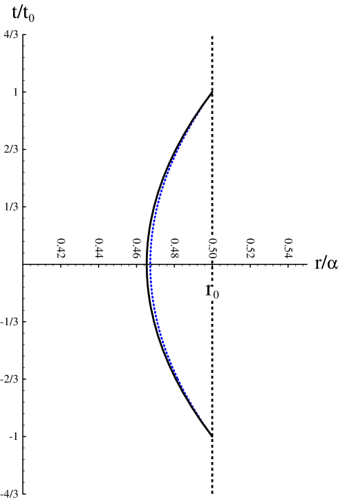
Figure 3.1: The exact geodesic path (dotted line) and the parabolic approximation (solid line) in de Sitter spacetime. The coordinate distance from $r=0$ to the horizon is $\alpha$ in the static coordinates.

The geodesic distance between two spacetime points, where the starting and ending spatial positions are the same, is given by

$$\Delta s=\int_{-t_{0}}^{+t_{0}}\sqrt{-|g_{tt}\left({\bf x}(t)\right)|+g_{ij}\left({\bf x}(t)\right){dx^{i}\over dt}{dx^{j}\over dt}}dt\,.$$ (3.47)

In order to carry out the integration, let us define

$$f(t)\equiv\sqrt{-|g_{tt}\left({\bf x}(t)\right)|+g_{ij}\left({\bf x}(t)\right){dx^{i}\over dt}{dx^{j}\over dt}}\,.$$ (3.48)

We can expand $f(t)$ in powers of $t$ centered around $t=0$, and then carry out the integration to find the geodesic distance. The parameter $\sigma$ can now be written as

$$\sigma({\bf x}_{0},t_{0}) = \sigma({\bf x}_{0},-t_{0};{\bf x}_{0},+t_{0})={1\over 2}\,{\Delta s}^{2}$$

$$= 2f^{2}(0)\,t_{0}^{2}+{2\over 3}f(0)f^{{}^{\prime\prime}}(0)\,t_{0}^{4}+{1\over 6}\left[{1\over 5}f(0)f^{(IV)}(0)+{1\over 3}f^{{}^{\prime\prime}}(0)^{2}\right]\,t_{0}^{6}+\cdots.$$

However, we do not know the values of the metric at the time $t=0$, but we do at the initial or final positions. Therefore, we expand the functions $f(0)$ around the time $-t_{0}$. Upon using Eq. (3.46), we find

$$\sigma({\bf x_{0}},t_{0})\approx-2|g_{tt}({\bf x_{0}})|\,t_{0}^{2}-{1\over 6}\,{g_{tt}}^{,i}({\bf x_{0}})\,g_{tt,i}({\bf x_{0}})\,t_{0}^{4}+\cdots,$$ (3.50)

and

$$\sigma^{t}({\bf x_{0}},t_{0})\approx 2t_{0}+{1\over 3}{{g_{tt}}^{,i}({\bf x_{0}})\,g_{tt,i}({\bf x_{0}})\over|g_{tt}({\bf x_{0}})|}\,t_{0}^{3}+\cdots.$$ (3.51)

In any further calculations, we will drop the ${\bf x_{0}}$ notation, with the understanding that all of the further metric elements are evaluated at the starting point of the geodesic. Using Eq. (3.21) we can then write the Euclidean Green’s function needed to derive the quantum inequality in increasing powers of $t_{0}$ as

$$G_{E}(x,t_{0}) = {1\over 8\pi^{2}}\left[{{1-O(t_{0}^{2})+\cdots}\over{2|g_{tt}|\,t_{0}^{2}-{1\over 6}{g_{tt}}^{,i}g_{tt,i}\,t_{0}^{4}}}+v_{0}\ln(2|g_{tt}|\,t_{0}^{2}-{1\over 6}{g_{tt}}^{,i}g_{tt,i}\,t_{0}^{4})\right.$$

$$+\left.\left(v_{0,k}\,|{g_{tt}}|^{,k}+2v_{1}|g_{tt}|-2v_{000}\right)t_{0}^{2}\ln(2|g_{tt}|\,t_{0}^{2}-{1\over 6}{g_{tt}}^{,i}g_{tt,i}\,t_{0}^{4})+\cdots\right].$$

Notice that none of the geometric terms, such as $v_{0}$, changes during Euclideanization because they are time independent. The quantum inequality, (3.23), can be written as

$$\Delta\hat{\rho}\geq-{1\over 4}\left({1\over|g_{tt}|}\partial_{t_{0}}^{2}+\nabla^{i}\nabla_{i}\right)\,G_{E}({\bf x},-t_{0};{\bf x},+t_{0}).$$ (3.53)

If we insert the Taylor series expansion for the Euclidean Green’s function into the above expression and collect terms in powers of the proper sampling time $\tau_{0}$, related to $t_{0}$ by $\tau_{0}=|g_{tt}|^{1/2}t_{0}$, we can write the above expression as

$$\Delta\hat{\rho} \geq -{3\over 32\pi^{2}\tau_{0}^{4}}\left[\rule{0.0pt}{18.06749pt}1+{1\over 3}\left({1\over 2}g_{tt}\,\nabla^{j}\nabla_{j}\;g_{tt}^{-1}+{1\over 6}R-m^{2}\right)\,\tau_{0}^{2}\right.$$

$$\qquad+{1\over 3}\left.\rule{0.0pt}{18.06749pt}\left({1\over 6}R_{,k}{{g_{tt}}^{,k}\over g_{tt}}-{1\over 12}\nabla^{j}\nabla_{j}\;R+4v_{1}-4{v_{000}\over|g_{tt}|}\right)\tau_{0}^{4}\ln(2\tau_{0}^{2})+O(\tau_{0}^{4})+\cdots\right].$$

In the limit of $\tau_{0}\rightarrow 0$, the dominant term of the above expression reduces to

$$\Delta\hat{\rho}\geq-{3\over 32\pi^{2}\tau_{0}^{4}}\,,$$ (3.55)

which is the quantum inequality in four-dimensional Minkowski space [32, 48]. Thus, the term in the square brackets in Eq. (LABEL:eq:QI_expansion) is the short sampling time expansion of the “scale” function [35], and does indeed reduce to one in the limit of the sampling time tending to zero. The range of sampling times for which a curved spacetime can be considered “roughly” flat is determined by the first non-zero correction term in Eq. (LABEL:eq:QI_expansion). If this happens to be the $\tau_{0}^{2}$ term, then for the first correction to be small compared to one implies

$$\tau_{0}\ll\left|{1\over 2}g_{tt}\,\nabla^{i}\nabla_{i}\;g_{tt}^{-1}+{1\over 6}R-m^{2}\right|^{-1/2}\,.$$ (3.56)

Each of the three terms on the right-hand side of this relation has a different significance. The $m^{2}$ term simply reflects that for a massive scalar field, Eq. (LABEL:eq:QI_expansion) is valid only when the sampling time is small compared to the Compton time. If we are interested in the massless scalar field, this term is absent. The scalar curvature term, if it is dominant, indicates that the flat space inequality is valid only on scales which are small compared to the local radius of curvature. This was argued on the basis of the equivalence principle by various authors [44, 40, 42], but is now given a more rigorous demonstration. The most mysterious term in Eq. (3.56) is that involving $g_{tt}$. Typically, this term dominates when the observer sits at rest near a spacetime horizon. In this case, the horizon acts as a boundary, so Eq. (3.56) requires $\tau_{0}$ to be small compared to the proper distance to the boundary.

In the particular case of $|g_{tt}|=1$, we have $\tau_{0}=t_{0}$ and Eq. (LABEL:eq:QI_expansion) reduces to

$$\Delta\hat{\rho}\geq-{3\over 32\pi^{2}t_{0}^{4}}\left[1+{1\over 3}\left({1\over 6}R-m^{2}\right)\,t_{0}^{2}+{1\over 3}\left(-{1\over 12}\nabla^{i}\nabla_{i}\;R+4v_{1}-4v_{000}\right)t_{0}^{4}\ln(2t_{0}^{2})+\cdots\right].$$ (3.57)

This result has also been obtained by Song [61], who uses a heat kernel expansion of the Green’s function to develop a short sampling time expansion. We can now apply Eq. (3.57) to a massless scalar field in the four-dimensional static Einstein universe. The metric is given by

$$ds^{2}=-dt^{2}+a^{2}\left[d\chi^{2}+\sin^{2}\chi(d\theta^{2}+\sin^{2}\theta d\varphi^{2})\right],$$ (3.58)

and the scalar curvature $R=6/a^{2}$ is a constant. It can be shown that $v_{1}-v_{000}=1/8a^{4}$. This leads to a quantum inequality in Einstein’s universe of the form

$$\Delta\hat{\rho}\geq-{3\over 32\pi^{2}t_{0}^{4}}\left[1+{1\over 3}\left({t_{0}\over a}\right)^{2}+{1\over 3}\left({t_{0}\over a}\right)^{4}\ln(t_{0}/a)+O({t_{0}^{4}\over a^{4}})+\cdots\right].$$ (3.59)

In Section 4.3.2, an exact quantum inequality valid for all $t_{0}/a$ will be derived. In the limit $t_{0}\ll a$, this inequality agrees with Eq. (3.59). Similarly, the exact inequality for the static, open Robertson-Walker universe will be obtained in Section 4.3.1, and in the limit $t_{0}\ll a$ agrees with Eq. (3.57).

3.4 Electromagnetic Field Quantum Inequality

In this section, we derive a quantum inequality for the quantized electromagnetic field in a static spacetime. It has been shown [62, 63] that the covariant Maxwell’s equations for the electromagnetic field in a curved spacetime,

$${F^{\mu\nu}}_{;\nu}=0$$ (3.60)

and

$$F_{\mu\nu;\sigma}+F_{\nu\sigma;\mu}+F_{\sigma\mu;\nu}=0\,,$$ (3.61)

can be recast into the form of Maxwell’s equations inside an anisotropic material medium in Cartesian coordinates, by using the constitutive relations

$$D_{i}=\epsilon_{ik}\,E_{k}-({\bf G}\times{\bf H})_{i}$$ (3.62)

and

$$B_{i}=\mu_{ik}H_{k}+({\bf G}\times{\bf E})_{i}\,,$$ (3.63)

where

$$\epsilon_{ik}=\mu_{ik}=-(-g)^{1/2}{g^{ik}\over g_{00}}\qquad{\rm and}\qquad G_{i}=-{g_{0i}\over g_{00}}\,.$$ (3.64)

Here the effects of the gravitational field are described by an anisotropic dielectric and permeable medium. However, when we consider the metric

$${ds}^{2}=-|g_{tt}({\bf x})|{dt}^{2}+g_{ij}({\bf x})dx^{i}dx^{j}\>,$$ (3.65)

there is considerable simplification. Because $g_{0i}=0$ for all $i$, the vector $G_{i}$ is always zero. The constitutive relations are then simply given by

$${\bf D}=\hat{\epsilon}\,{\bf E}\qquad{\rm and}\qquad{\bf B}=\hat{\epsilon}\,{\bf H},$$ (3.66)

where

$$\hat{\epsilon}=\hat{\epsilon}({\bf x})={\sqrt{-g}\over|g_{tt}|}\left(\begin{array}[]{lll}g^{11}&g^{12}&g^{13}\\ g^{21}&g^{22}&g^{23}\\ g^{31}&g^{32}&g^{33}\end{array}\right)\,.$$ (3.67)

The source-free Maxwell equations, in terms of $({\bf E},{\bf H})$, are given by

$$\nabla\times{\bf E}=-{\partial\,{\bf B}\over\partial t}\,,\quad \quad\nabla\cdot{\bf D}=0\,,$$ (3.68)

$$\nabla\times{\bf H}={\partial\,{\bf D}\over\partial t}\,,\quad \quad\nabla\cdot{\bf B}=0\,.$$ (3.69)

We may also define the source-free vector potential $A_{\mu}({\bf x},t)=(0,{\bf A})$ with the relations to the electric and magnetic fields given by

$${\bf E}=-{\partial\,{\bf A}\over\partial t}\qquad\mbox{ and }\qquad{\bf B}=\nabla\times{\bf A}.$$ (3.70)

It is straightforward to show that the vector potential satisfies the wave equation

$$\hat{\epsilon}^{-1}\nabla\times\hat{\epsilon}^{-1}(\nabla\times{\bf A})=-{\partial^{2}\,{\bf A}\over\partial t^{2}}\,.$$ (3.71)

The left-hand side of Eq. (3.71) involves only derivatives with respect to the position coordinates, and the right-hand side, temporal derivatives. This is a clear separation of variables, allowing us to write the positive frequency solutions as

$${\bf f}_{\bf k}^{\lambda}({\bf x},t)={\bf U}_{\bf k}^{\lambda}({\bf x})\;e^{-i\omega t},$$ (3.72)

where ${\bf k}$ is the mode label for the propagation vector and $\lambda$ is the polarization state. The vector functions, ${\bf U}_{\bf k}^{\lambda}({\bf x})$, are the solutions of

$$\hat{\epsilon}^{-1}\nabla\times\hat{\epsilon}^{-1}(\nabla\times{\bf U}_{\bf k}^{\lambda})-\omega^{2}{\bf U}_{\bf k}^{\lambda}=0,$$ (3.73)

and carry all the information about the curvature of the spacetime. The mode functions for the vector potential are normalized such that

$$\left({\bf f}_{\bf k}^{\lambda},{\bf f}_{\bf k^{\prime}}^{\lambda^{\prime}}\right)=-i\int d^{3}x\left[{\bf f}_{\bf k}^{\lambda}\cdot\partial_{t}{{\bf f}_{\bf k^{\prime}}^{\lambda^{\prime}}}^{*}-(\partial_{t}{\bf f}_{\bf k}^{\lambda})\cdot{{\bf f}_{\bf k^{\prime}}^{\lambda^{\prime}}}^{*}\right]=\delta_{\bf kk^{\prime}}\delta_{\lambda\lambda^{\prime}}\,.$$ (3.74)

The general solution to the vector potential can then be expanded as

$${\bf A}({\bf x},t)=\sum_{{\bf k},\lambda}\left(a_{{\bf k}\lambda}{\bf U}_{\bf k}^{\lambda}({\bf x})e^{-i\omega t}+a_{{\bf k}\lambda}^{\dagger}{{\bf U}_{\bf k}^{\lambda}}^{*}({\bf x})e^{+i\omega t}\right)\,.$$ (3.75)

When we go to second quantization, the coefficients, $a_{{\bf k}\lambda}^{\dagger}$ and $a_{{\bf k}\lambda}$ become the creation and annihilation operators for the photon. We will again develop the quantum inequality for the electromagnetic field for a static observer, as was done above for the scalar field. The observed energy density, $\rho$, is given by [63]

$$\rho={1\over 2}(-g)^{-1/2}\left({\bf E\cdot D}+{\bf B\cdot H}\right).$$ (3.76)

Upon substitution of the mode function expansion, and making use of constitutive relations (3.66) we find

$$\rho = {1\over|g_{tt}|}\,{\rm Re}\!\!\sum_{{\bf k\,k^{\prime}},\lambda\lambda^{\prime}}\omega\omega^{\prime}\left[a_{{\bf k}\lambda}^{\dagger}a_{{\bf k}^{\prime}\lambda^{\prime}}\>({{\bf U}_{\bf k}^{\lambda}}_{i}^{*}\;g^{ij}\;{{\bf U}_{{\bf k}^{\prime}}^{\lambda^{\prime}}}_{j})\,e^{i(\omega-\omega^{\prime})t}-a_{{\bf k}\lambda}a_{{\bf k}^{\prime}\lambda^{\prime}}\>({{\bf U}_{\bf k}^{\lambda}}_{i}\;g^{ij}\;{{\bf U}_{{\bf k}^{\prime}}^{\lambda^{\prime}}}_{j})\,e^{-i(\omega+\omega^{\prime})t}\right]$$ (3.77)

$$+|g_{tt}|\,{\rm Re}\!\!\sum_{{\bf k\,k^{\prime}},\lambda\lambda^{\prime}}\left[a_{{\bf k}\lambda}^{\dagger}a_{{\bf k}^{\prime}\lambda^{\prime}}\>(\nabla\times{{\bf U}_{\bf k}^{\lambda}}^{*})_{i}\;g^{ij}\;(\nabla\times{\bf U}_{{\bf k}^{\prime}}^{\lambda^{\prime}})_{j}\,e^{i(\omega-\omega^{\prime})t}\right.$$

$$\left.\qquad\qquad+a_{{\bf k}\lambda}a_{{\bf k}^{\prime}\lambda^{\prime}}\>(\nabla\times{\bf U}_{\bf k}^{\lambda})_{i}\;g^{ij}\;(\nabla\times{\bf U}_{{\bf k}^{\prime}}^{\lambda^{\prime}})_{j}\,e^{-i(\omega+\omega^{\prime})t}\right]$$

$$+{1\over 2}\sum_{{\bf k},\lambda}\left[{\omega^{2}\over|g_{tt}|}({{\bf U}_{\bf k}^{\lambda}}_{i}\;g^{ij}\;{{\bf U}_{\bf k}^{\lambda}}_{j}^{*})+|g_{tt}|\>(\nabla\times{\bf U}_{\bf k}^{\lambda})_{i}\;g^{ij}\;(\nabla\times{{\bf U}_{\bf k}^{\lambda}}^{*})_{j}\right].$$

The last term of the above expression is the vacuum self-energy of the photons. As was the case for the scalar field, we will look at the difference between the energy in an arbitrary state and the vacuum energy, i.e.,

$$:\rho:=\rho-\langle 0|\rho|0\rangle.$$ (3.78)

Again we integrate the energy density along the worldline of the observer, weighted by the Lorentzian sampling function. We may then apply the first inequality, Eq. (3.14) proven in [48]. To the result we apply the inequality proven in Appendix A. We then find that the difference inequality on the energy density for a quantized electromagnetic field is given by

$$\Delta\hat{\rho}\geq-{1\over 2}\sum_{{\bf k},\lambda}\left[{\omega^{2}\over|g_{tt}|}({{\bf U}_{\bf k}^{\lambda}}_{i}\;g^{ij}\;{{\bf U}_{\bf k}^{\lambda}}_{j}^{*})+|g^{tt}|\>(\nabla\times{\bf U}_{\bf k}^{\lambda})_{i}\;g^{ij}\;(\nabla\times{{\bf U}_{\bf k}^{\lambda}}^{*})_{j}\right]e^{-2\omega t_{0}}.$$ (3.79)

This expression is similar in form to the mode function expansion of the scalar field quantum inequality, and also reduces to an averaged weak energy type integral in the infinite sampling time limit. As was the case for the scalar field, the electromagnetic field quantum inequality (3.79) tells us how much negative energy an observer may measure with respect to the vacuum energy of the electromagnetic field. In order to find the absolute lower bound on the negative energy density we would have to add the renormalized vacuum energy into the above expression.

This quantum inequality can be easily evaluated in Minkowski spacetime. In a box of volume $L^{3}$ with periodic boundary conditions, the mode functions are given by

$${{\bf U}_{\bf k}^{\lambda}}=\left(2\omega L^{3}\right)^{1/2}\,e^{i{\bf k\cdot x}}\,\hat{\epsilon}_{\bf k}^{\lambda},$$ (3.80)

where $\hat{\epsilon}_{\bf k}^{\lambda}$ is a unit polarization vector and $\omega=\sqrt{\bf k\cdot k}$. Inserting the mode functions into Eq. (3.79), and using the fact that ${\bf k}\cdot\hat{\epsilon}_{\bf k}^{\lambda}=0$, we find

$$\Delta\hat{\rho}\geq-{1\over 2L^{3}}\sum_{{\bf k},\lambda}\omega\,e^{-2\omega t_{0}}.$$ (3.81)

The summation over the spin degrees of freedom yields

$$\Delta\hat{\rho}\geq-{1\over L^{3}}\sum_{\bf k}\omega\,e^{-2\omega t_{0}}.$$ (3.82)

In the continuum limit, $L\rightarrow\infty$, the vacuum energy density vanishes, and the renormalized quantum inequality is found to be

$$\hat{\rho} \geq -{1\over(2\pi)^{3}}\int_{-\infty}^{\infty}d^{3}k\>\omega\,e^{-2\omega t_{0}},$$ (3.83)

$$= -{3\over 16\pi^{2}\,t_{0}^{4}}.$$

This quantum inequality for Minkowski spacetime was originally proven by Ford and Roman [48] using an alternative method. Comparison with the quantum inequality for the scalar field in Minkowski space, Eq. (1.13), shows that the electromagnetic field quantum inequality differs by a factor of 2. This is a result of the electromagnetic field having two polarization degrees of freedom, unlike the scalar field which has only one.

Chapter 4 Scalar Field Examples

4.1 Two-Dimensional Spacetimes

There are a number of interesting results for two-dimensional spacetimes that we will discuss. The unique conformal properties in two dimensions allow the quantum inequality for all two-dimensional static spacetimes to be written in the form

$$\Delta\hat{\rho}\geq-{1\over 8\pi\tau_{0}^{2}}\,,$$ (4.1)

where $\tau_{0}$ is the proper time of the stationary observer. Similarly, the quantum inequality for the flux traveling in one direction is

$$\hat{f}\equiv{t_{0}\over\pi}\int_{-\infty}^{\infty}{\langle T^{xt}\rangle\over t^{2}+t_{0}^{2}}\,dt\,\geq-{1\over 16\pi t_{0}^{2}}\,.$$ (4.2)

We emphasize that these results are only for static two-dimensional spacetimes. The original derivation of the quantum inequality of the preceding chapter relies on the metric having a natural choice of a timelike Killing vector field. This allows us to clearly define the notion of positive frequency for the mode functions. The conformal property of two-dimensional spacetimes is more general than the quantum inequality, in that even spacetimes which are time evolving will be conformal to some part of two-dimensional Minkowski spacetime.

Recently, Flanagan [64] has demonstrated another interesting aspect of the quantum inequalities in two-dimensional spacetimes. He has shown that a general form of the quantum inequality can be developed in two-dimensional Minkowski spacetime which is independent of the choice of the sampling function. We will summarize his results below, but first we will look at the conformal triviality of all static two-dimensional spacetimes.

4.1.1 Conformal Properties

It is a unique property of two-dimensional spacetimes that any metric can be cast into the form

$$g_{\mu\nu}(x)\,\rightarrow\,g_{\mu\nu}(y)=\Omega^{2}(y)\eta_{\mu\nu}$$ (4.3)

by choosing an appropriate coordinate transform, $x\rightarrow y=y(x)$. For the massless scalar field, the wave equation

$$\mathord{\hbox{\Bxfnt\char 116\relax}\hbox to0.0pt{\hss\Bxfnt\char 117\relax}}\phi(x)=0$$ (4.4)

then becomes

$$\Omega^{-2}(y)\eta^{\mu\nu}\partial_{\mu}\partial_{\nu}\bar{\phi}(y)=0.$$ (4.5)

The mode functions in the two different coordinates are related by

$$\phi(x)=\bar{\phi}(y(x)).$$ (4.6)

However, $\bar{\phi}(y)$ is the scalar field solution to the wave equation in Minkowski spacetime, composed from the standard mode functions

$$\bar{f}_{k}(y)=(4\pi\omega)^{-1/2}e^{ik\cdot y}\,,$$ (4.7)

where $k_{0}=\omega=|k_{1}|$. In two dimensions, the Green’s functions are found to transform as

$$D(x,x^{\prime})=\bar{D}(y(x),y(x^{\prime}))\,,$$ (4.8)

where $\bar{D}(y,y^{\prime})$ is the standard Minkowski Green’s functions. For example, the Wightman Green’s function in two-dimensional Minkowski spacetime is

$$D^{+}(y,y^{\prime})=\langle 0|\bar{\phi}(y)\bar{\phi}(y^{\prime})|0\rangle={1\over 4\pi}\int_{-\infty}^{\infty}{dk\over\omega}e^{ik\cdot(y-y^{\prime})}\,.$$ (4.9)

This would also be the Wightman Green’s function in an arbitrary curved two-dimensional spacetime expressed in the coordinates chosen from the metric (4.3). It is evident from the expression above that the massless Green’s functions have an infrared divergence. It is possible to carry out the integration of the above Green’s function, and renormalize away the infrared divergence. However, for our purposes, the integral representation is sufficient.

We have already shown for static spacetimes that the QI is given by

$$\Delta\hat{\rho}\geq-{1\over 4}\mathord{\hbox{\Bxfnt\char 116\relax}\hbox to0.0pt{\hss\Bxfnt\char 117\relax}}_{E}D_{E}(x,-it_{0};x,+it_{0}).$$ (4.10)

If we now make use of the conformal relations for the box operator and the Green’s function, we find

$$\Delta\hat{\rho}\geq-{1\over 4}\Omega^{-2}(y)\bar{\mathord{\hbox{\Bxfnt\char 116\relax}\hbox to0.0pt{\hss\Bxfnt\char 117\relax}}}_{E}\bar{D}_{E}(y,-it_{0};y,+it_{0})=-{1\over 16\pi}\Omega^{-2}(y)\partial^{2}_{t_{0}}\int_{-\infty}^{\infty}{dk\over\omega}e^{-2\omega t_{0}}.$$ (4.11)

We see that while the Green’s function has an infrared divergence, the quantum inequality does not. We can interchange the order of the integration and differentiation with the resulting integral being well defined for all values of $k$, and find

$$\Delta\hat{\rho}\geq-{1\over 8\pi\left[\Omega(y)t_{0}\right]^{2}}\,.$$ (4.12)

However, in static spacetimes the coordinate time and the proper time of an observer are related by $\tau_{0}=\Omega(y)t_{0}$. We can then write the quantum inequality in a more covariant form as

$$\Delta\hat{\rho}\geq-{1\over 8\pi\tau_{0}^{2}}\,.$$ (4.13)

This is exactly the form of the quantum inequality found by Ford and Roman in Minkowski spacetime [32]. The difference inequality above is applicable to all static two-dimensional spacetimes. However the renormalized quantum inequalities in any two-dimensional spacetimes will be different because the vacuum energies in these spacetimes are not identical. We can write the renormalized two-dimensional quantum inequality as

$$\hat{\rho}_{Ren.}\geq-{1\over 8\pi\tau_{0}^{2}}+\rho_{vacuum},$$ (4.14)

where $\rho_{vacuum}$ is the vacuum energy that is defined with respect to the timelike Killing vector field.

4.1.2 Sampling Functions in Two-Dimensional Spacetimes

In the previous chapter, we have proven quantum inequalities using the Lorentzian sampling function, Eq. (3.12). The Lorentzian was chosen to facilitate the proof of the inequality. Recently, Flanagan [64] has shown that quantum inequalities for the massless scalar field in two-dimensional Minkowski spacetime can be developed for arbitrary sampling functions. (Note: Flanagan uses the term “smearing functions.”) We summarize his results below.

We begin with a smooth, nonnegative function $f(v)$ with unit normalization,

$$\int_{-\infty}^{\infty}\,f(v)\,dv=1.$$ (4.15)

It is not necessary that the sampling function have compact support so long as the function approaches zero sufficiently quickly to ensure convergence of the above integral. Using the stress-tensor in the standard $(x,t)$ coordinates, we define three smeared integral quantities: the time-smeared energy density

$$\Delta\hat{\rho}={\cal E}_{T}\equiv\int_{-\infty}^{\infty}dt\,f(t)\,\langle:T_{tt}(0,t):\rangle,$$ (4.16)

the time-smeared flux

$$\Delta\hat{F}={\cal E}_{F}\equiv\int_{-\infty}^{\infty}dt\,f(t)\,\langle:T^{xt}(0,t):\rangle,$$ (4.17)

and the spatially-smeared energy density

$${\cal E}_{S}\equiv\int_{-\infty}^{\infty}dx\,f(x)\,\langle:T_{tt}(x,0):\rangle.$$ (4.18)

Flanagan then shows that all three of the above integral quantities are bounded below by

$${\cal E}_{T,min}={\cal E}_{S,min}=2{\cal E}_{F,min}=-{1\over 24\pi}\int_{-\infty}^{\infty}dv\,{f^{\prime}(v)^{2}\over f(v)}.$$ (4.19)

This is achieved by use of a Bogolubov transformation which converts the quadratic form of the integral in Eq. (4.16) into a simple form. (Details of the proof can be found in [64].) Flanagan also shows that this is an optimum lower bound for a given sampling function. This lower bound is achieved by the vacuum state associated with the new coordinates used in the Bogolubov transform. This new vacuum state is a generalized multi-mode squeezed state of the original vacuum defined in the $(x,t)$ coordinates.

For arbitrary sampling functions, it is now straightforward to find the optimum quantum inequality in two-dimensional Minkowski spacetime. For example, if we use the Lorentzian sampling function, Eq. (3.12), in the time-smeared energy density, we find

$$\Delta\hat{\rho}\geq-{1\over 48\pi t_{0}^{2}}\,.$$ (4.20)

This is six times more restrictive than the quantum inequality derived in the preceding section. We knew that the quantum inequality developed using the Green’s function was a lower bound, but it was not necessarily known if it was the optimum lower bound. We now see that Eq. (4.20) represents the optimum quantum inequality for the Lorentzian sampling function.

4.2 Three-Dimensional Spacetimes

We now discuss examples of three-dimensional spacetimes in which it is straightforward to find the quantum inequalities. First we will develop the quantum inequality in Minkowski spacetime for a massive scalar field. The addition of the mass makes the quantum inequality more restrictive. In order to generate negative energy densities, we must overcome both the momentum of the particle and its rest mass. We will then look at the three-dimensional equivalent of the static Einstein universe. Unlike the two-dimensional examples of the preceding section, we will see that in three dimensions the form of the quantum inequality is modified from its flat space form because of the spacetime curvature. In addition, we will be able to renormalize the quantum inequality in the three-dimensional closed universe. Here there exists a non-zero vacuum energy that must be taken into consideration. In this case the quantum inequality tells us how much negative energy we can measure relative to the background vacuum energy.

4.2.1 Minkowski Spacetime

We begin with the easiest example, three-dimensional flat spacetime, where we know that the positive frequency massive mode functions are given by

$$f_{\bf k}(x,y,t)=[2\omega(2\pi)^{2}]^{-1/2}e^{i{\bf k}\cdot{\bf x}-i\omega t}\,,$$ (4.21)

with a frequency $\omega=\sqrt{|\bf k|^{2}+\mu^{2}}$ and $-\infty<k_{i}<\infty$. The required two-point function is then defined by

$$G_{E}(2t_{0})=\int_{-\infty}^{\infty}dk_{x}\,dx_{y}\;\left|{1\over\sqrt{2\omega(2\pi)^{2}}}e^{i{\bf k}\cdot{\bf x}}\right|^{2}e^{-2\omega t_{0}}\,.$$ (4.22)

It is rather straightforward to carry out the required integrations to find

$$G_{E}(2t_{0})={1\over 8\pi t_{0}}\,e^{-2mt_{0}}.$$ (4.23)

Now the difference inequality is given by Eq. (3.23), where the Euclidean box operator is

$$\mathord{\hbox{\Bxfnt\char 116\relax}\hbox to0.0pt{\hss\Bxfnt\char 117\relax}}_{E}=\partial_{t_{0}}^{2}+\partial_{x}^{2}+\partial_{y}^{2}\,.$$ (4.24)

One thing that should be pointed out before proceeding is that the vacuum energy in three-dimensional Minkowski spacetime is defined to be zero. Under such circumstances, we are placing a lower bound on the energy density of the state itself, and not just on the difference of the energy density between the state and the vacuum energy. The quantum inequality becomes

$$\hat{\rho}\geq-{1\over 32\pi}\partial_{t_{0}}^{2}\left[{1\over t_{0}}\,e^{-2\mu t_{0}}\right]\,,$$ (4.25)

which upon taking the time derivatives can be written as

$$\hat{\rho}\geq-{1\over 16\pi t_{0}^{3}}S(2\mu t_{0})\,.$$ (4.26)

The “scale function,” $S(x)$, is defined as

$$S(x)=\left(1+x+{1\over 2}x^{2}\right)\,e^{-x}\,.$$ (4.27)

The scale function represents modifications to the quantum inequality due to the mass of the the particle. It is plotted in Figure 4.1. When $\mu=0$, the scale function becomes one and the quantum inequality reduces to the massless form

$$\hat{\rho}\geq-{1\over 16\pi t_{0}^{3}}\,.$$ (4.28)

This is what would have been found if we had chosen the massless mode functions at the beginning of this derivation. It is interesting to note that in the limit of the mass of the scalar particle becoming very large, the scale function will tend to zero. Thus, if the particle has a mass, it becomes more difficult to observe negative energy densities.

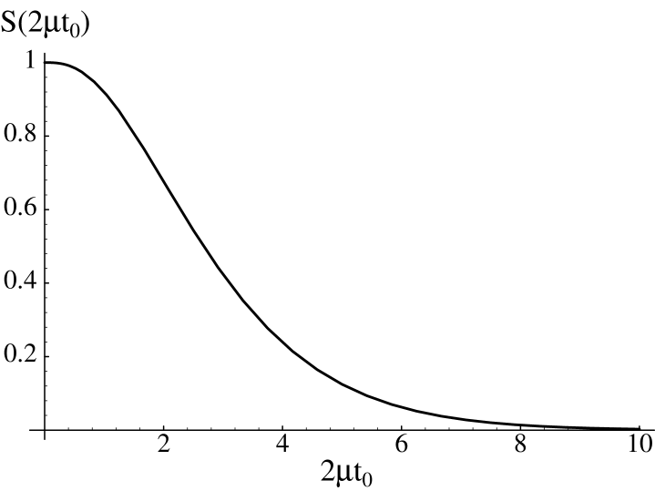
Figure 4.1: The scale function $S(2\mu t_{0})$ for three-dimensional Minkowski spacetime.

Since the mode functions are invariant under Lorentz transformations, we can always choose to develop the inequality in the observer’s rest frame and then transform to any other frame. The quantum inequality can therefore be written in a more covariant form in flat spacetime as

$$\hat{\rho}\,\equiv\,{\tau_{0}\over\pi}{\int_{-\infty}^{\infty}}{\langle:T_{\alpha\beta}u^{\alpha}u^{\beta}:\rangle\over{\tau^{2}+\tau_{0}^{2}}}d\tau\,\geq\,-{1\over 16\pi\tau_{0}^{3}}\,S(2\mu\tau_{0}).$$ (4.29)

Here $\tau$ is the observer’s proper time, $\tau_{0}$ is the sampling time, and $u^{\alpha}=d\,x^{\alpha}(\tau)/d\tau$ is the observer’s four-velocity.

4.2.2 The Closed Universe

Let us consider the three-dimensional spacetime with a length element given by

$$ds^{2}=-dt^{2}+a^{2}\left(d\theta^{2}+\sin^{2}\theta d\varphi^{2}\right).$$ (4.30)

Here constant time-slices of this universe are two spheres of radius $a$. The wave equation on this background with a coupling of strength $\xi$ to the Ricci scalar $R$ is

$$\mathord{\hbox{\Bxfnt\char 116\relax}\hbox to0.0pt{\hss\Bxfnt\char 117\relax}}\phi-(\mu^{2}+\xi R)\phi=0.$$ (4.31)

For the metric (4.30), the wave equation becomes

$$-\partial_{t}^{2}\phi+{1\over{a^{2}\sin\theta}}\partial_{\theta}\left(\sin\theta\partial_{\theta}\phi\right)+{1\over{a^{2}\sin^{2}\theta}}\partial_{\varphi}^{2}\phi-[\mu^{2}+\xi\left(2\over a^{2}\right)]\phi=0,$$ (4.32)

which has the solutions

$$f_{lm}(t,\theta,\varphi)={1\over{\sqrt{2a^{2}\omega}}}{\rm Y}_{lm}(\theta,\varphi)e^{-i\omega_{l}t}.$$ (4.33)

The ${\rm Y}_{lm}$ are the usual spherical harmonics with unit normalization. The mode labels take the values, $l=0,1,2,\cdots$ and $-l\leq m\leq l$. For each state of the primary quantum number $l$, there is a degeneracy of $2l+1$ associated with the $m$, each having the same eigenfrequency

$$\omega_{l}=a^{-1}\sqrt{l(l+1)+2\xi+\mu^{2}a^{2}}\,.$$ (4.34)

The coupling parameter $\xi$ here can be seen to contribute to the wave functions as a term of the same form as the mass. However, we will look only at minimal coupling ($\xi=0$). The lower bound on the energy density is given by

$$\Delta\hat{\rho}\geq-{1\over{2a^{2}}}\sum_{l=0}^{\infty}\sum_{m=-l}^{+l}\omega_{l}|{\rm Y}_{lm}(\theta,\varphi)|^{2}e^{-2\omega_{l}t_{0}}-{1\over 8a^{2}}\nabla^{i}\nabla_{i}\sum_{l=0}^{\infty}\sum_{m=-l}^{+l}{1\over\omega_{l}}|{\rm Y}_{lm}(\theta,\varphi)|^{2}e^{-2\omega_{l}t_{0}}.$$ (4.35)

However the spherical harmonics obey a sum rule [65]

$$\sum_{m=-l}^{+l}|{\rm Y}_{lm}(\theta,\varphi)|^{2}={{2l+1}\over{4\pi}}.$$ (4.36)

We immediately see that the difference inequality is independent of position, as expected from the spatial homogeneity, and that the second term of Eq. (4.35) does not contribute. We have

$$\Delta\hat{\rho}\geq-{1\over{8\pi a^{2}}}\sum_{l=0}^{\infty}(2l+1)\,\omega_{l}e^{-2\omega_{l}t_{0}}.$$ (4.37)

This summation is finite due to the exponentially decaying term. We are now left with evaluating the sum for a particular set of values for the mass $\mu$, the radius $a$, and the sampling time $t_{0}$. Let $\eta={t_{0}/a}$. Then

$$\Delta\hat{\rho}\geq-{1\over{16\pi t_{0}^{3}}}\left[2\eta^{3}\sum_{l=1}^{\infty}(2l+1)\,\tilde{\omega}_{l}\,{\rm e}^{-2\eta\tilde{\omega}_{l}}\right]=-{1\over{16\pi t_{0}^{3}}}F(\eta,\mu),$$ (4.38)

where

$$\tilde{\omega}_{l}=\sqrt{l(l+1)+a^{2}\mu^{2}}\,.$$ (4.39)

The coefficient $-{1/(16\pi t_{0}^{3})}$ is the right-hand side of the inequality for the case of a massless field in an infinite three-dimensional Minkowski space. The “scale function,” $F(\eta,\mu)$, represents how the mass and the curvature of the closed spacetime affects the difference inequality.

4.2.3 Massless Case

In terms of the variable $\eta={t_{0}/a}$, which is the ratio of the sampling time to the radius of the universe, we can write the above expression for $F(\eta,0)$ as

$$F(\eta)=F(\eta,0)=2\eta^{3}\sum_{l=1}^{\infty}(2l+1)\sqrt{l(l+1)}\,{\rm e}^{-2\eta\sqrt{l(l+1)}}.$$ (4.40)

A plot of $F(\eta)$ is shown in Figure 4.2. In the limit of $\eta\rightarrow 0$, when the sampling time is very small or the radius of the universe has become so large that it approximates flat space, the function $F(\eta)$ approaches one, yielding the flat space inequality.

We can look at the inequality in the two asymptotic regimes of $\eta$. In the large $\eta$ regime each term of greater $l$ in the exponent will decay faster than the previous term. The $l=1$ term yields a good approximation. In the other regime, when the sampling time is small compared to the radius, we can use the Plana summation formula to calculate the summation explicitly:

$$\sum_{n=1}^{\infty}f(n)+{1\over 2}f(0)=\int_{0}^{\infty}f(x)dx+i\int_{0}^{\infty}{f(ix)-f(-ix)\over{{\rm e}^{2\pi x}-1}}dx\,,$$ (4.41)

where

$$f(x)=(2x+1)\sqrt{x(x+1)}\,{\rm e}^{-2\eta\sqrt{x(x+1)}}.$$ (4.42)

Immediately we see that for our summation $f(0)=0$. The first integral can be done with relative ease yielding

$$\int_{0}^{\infty}f(x)dx=\int_{0}^{\infty}(2x+1)\sqrt{x(x+1)}\,{\rm e}^{-2\eta\sqrt{x(x+1)}}dx=\frac{1}{2\eta^{3}}\,.$$ (4.43)

This term reproduces the flat space inequality. The second integral in Eq. (4.41) therefore contains all the corrections due to non-zero curvature of the spacetime. Since $\eta$ is small, we can expand the exponent in a Taylor series around $\eta=0$. Keeping the lowest order terms, we find

$$i\int_{0}^{\infty}{f(ix)-f(-ix)\over{e^{2\pi x}-1}}dx\sim-I_{0}-\eta I_{1}+\cdots\,,$$ (4.44)

where

$$I_{0}=\int_{0}^{\infty}\sqrt{2x}\;{\left(2x\sqrt{\sqrt{x^{2}+1}-x}+\sqrt{\sqrt{x^{2}+1}+x}\right)\over{{\rm e}^{2\pi x}-1}}\;dx\approx 0.265096,$$ (4.45)

and

$$I_{1}=\int_{0}^{\infty}{4x(2x^{2}-1)\over{{\rm e}^{2\pi x}-1}}dx=-\frac{2}{15}\,.$$ (4.46)

Therefore the function $F(\eta)$ in the small $\eta$ limit is given by

$$F(\eta)\simeq 1-0.530192\,\eta^{3}+{4\over 15}\eta^{4}+O(\eta^{5})+\cdots\,,$$ (4.47)

and in the large $\eta$ limit by

$$F(\eta)\simeq 6\sqrt{2}\,\eta^{3}\,{\rm e}^{-2\sqrt{2}\eta}+\cdots\,.$$ (4.48)

Both of these asymptotic forms are plotted along with the exact form of $F(\eta)$ in Figure 4.2. The graph shows that the

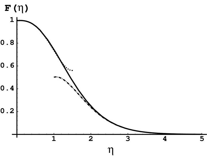
Figure 4.2: The scale function $F(\eta)$ and its asymptotic forms for the three-dimensional closed universe. The solid line is the exact form of the function. The dotted line is the small $\eta$ approximation, while the dot-dash line is the large $\eta$ approximation.

two asymptotic limits follow the exact graph very precisely except in the interval $1<\eta<2$. These results for the function $F(\eta)$, combined with Eq. (4.38), yield the difference inequality for the massless scalar field.

The difference inequality does not require knowledge of the actual value of the renormalized vacuum energy, $\rho_{vacuum}$. However, if we wish to obtain a bound on the energy density itself, we must combine the difference inequality and $\rho_{vacuum}$. One procedure for computing $\rho_{vacuum}$ is analogous to that used to find the Casimir energy in flat spacetime with boundaries: One defines a regularized energy density, subtracts the corresponding flat space energy density, and then takes the limit in which the regulator is removed. A possible choice of regulator is to insert a cutoff function, $g(\omega)$, in the mode sum and define the regularized energy density as

$$\rho_{reg}=\frac{1}{8\pi a^{2}}\sum_{\lambda}\omega_{\lambda}\,g(\omega_{\lambda})=\frac{1}{8\pi a^{2}}\sum_{l=0}^{\infty}(2l+1)\,\omega_{l}\,g(\omega_{l})\,.$$ (4.49)

In the limit that $a\rightarrow\infty$, we may replace the sum by an integral and obtain the regularized flat space energy density:

$$\rho_{FSreg}=\frac{1}{4\pi}\int_{0}^{\infty}{\rm d}\omega\,\omega\,g(\omega)\,.$$ (4.50)

The renormalized vacuum energy density may then be defined as

$$\rho_{vacuum}=\lim_{g\rightarrow 1}(\rho_{reg}-\rho_{FSreg})\,.$$ (4.51)

The vacuum energy density so obtained will be denoted by $\rho_{Casimir}$. An analogous procedure was used in [13] to obtain the vacuum energy density for the conformal scalar field in the four-dimensional Einstein universe. An explicit calculation for the present case, again using the Plana summation formula, yields

$$\rho_{Casimir}=-{I_{0}\over{8\pi a^{3}}}\approx-{0.265096\over{8\pi a^{3}}}.$$ (4.52)

This agrees with the result obtained by Elizalde [15] using the zeta function technique. In this case $\rho_{Casimir}<0$, whereas the analogous calculation for the conformal scalar field in this three-dimensional spacetime yields a positive vacuum energy density, $\rho_{Casimir}=1/{96\pi a^{3}}$. It should be noted that this procedure works for the closed universe because the divergent part of $\rho_{reg}$ is independent of $a$. More generally, there may be curvature-dependent divergences which must also be removed.

Let us now return to the explicit forms of the difference inequality. In the limit that $t_{0}\gg a$, Eqs. (4.38) and (4.48) yield

$$\Delta\hat{\rho}\geq-{{3\sqrt{2}}\over{8\pi a^{3}}}\,{\rm e}^{-2\sqrt{2}\,t_{0}/a}\,.$$ (4.53)

Similarly, in the limit that $t_{0}\ll a$, we find

$$\Delta\hat{\rho}\geq-{1\over{16\pi t_{0}^{3}}}-\rho_{Casimir}-{{t_{0}}\over{60\pi a^{4}}}+\cdots\,.$$ (4.54)

Thus the bound on the renormalized energy density in an arbitrary quantum state in the latter limit becomes

$$\hat{\rho}_{Ren.}\geq-{1\over{16\pi t_{0}^{3}}}-{{t_{0}}\over{60\pi a^{4}}}+\cdots\,.$$ (4.55)

In the $a\rightarrow\infty$ limit, both Eqs. (4.54) and (4.55) reduce to the quantum inequality for three-dimensional Minkowski space, Eq. (4.28). In this limit $\rho_{Casimir}=0$ so $\Delta\hat{\rho}=\hat{\rho}$. In the other limit when the sampling time becomes long, we find that $\Delta\hat{\rho}$ decays exponentially as a function of the sampling time. This simply reflects the fact that the difference in energy density between an arbitrary state and the vacuum state satisfies the quantum averaged weak energy condition, Eq. (1.11).

4.3 Four-Dimensional Robertson-Walker Universe

Now we will apply the same method to the case of the three homogeneous and isotropic universes given by the four-dimensional static Robertson-Walker metrics. Here we have

$$[\epsilon=0]:\qquad g_{ij}dx^{i}dx^{j}=dx^{2}+dy^{2}+dz^{2},$$ (4.56)

for the flat universe with no curvature (Minkowski spacetime). For the closed universe with constant radius $a$, i.e., the universe of constant positive curvature, the spatial length element is given by

$$[\epsilon=1]:\qquad g_{ij}dx^{i}dx^{j}=a^{2}\left[d\chi^{2}+\sin^{2}\chi(d\theta^{2}+\sin^{2}\theta d\varphi^{2})\right]\,,$$ (4.57)

where $0\leq\chi\leq\pi$, $0\leq\theta\leq\pi$, and $0\leq\varphi<2\pi$. The open universe $[\epsilon=-1]$ is given by making the replacement $\sin\chi\rightarrow\sinh\chi$ in Eq. (4.57) and now allowing $\chi$ to take on the values $0\leq\chi<\infty$. To find the lower bound of the quantum inequalities above we must solve for the eigenfunctions of the covariant Helmholtz equation

$$\nabla_{i}\nabla^{i}U_{\lambda}({\bf x})+(\omega^{2}_{\lambda}-\mu^{2})U_{\lambda}({\bf x})=0,$$ (4.58)

where $\mu$ is the mass of the scalar field and $\omega_{\lambda}$ is the energy. A useful form of the solutions for this case is given by Parker and Fulling [66].

4.3.1 Flat and Open Universes in Four Dimensions

In the notation developed in Chapter 3, the spatial portion of the wave functions for flat (Euclidean) space is given by (continuum normalization)

$$[\epsilon=0]:\qquad\quad U_{\bf k}({\bf x}) = [2\omega(2\pi)^{3}]^{-1/2}e^{i{\bf k}\cdot{\bf x}},$$ (4.59)

$$\omega = \sqrt{|\bf k|^{2}+\mu^{2}}\,,$$ (4.60)

$${\bf k} = (k_{1},k_{2},k_{3})\qquad(-\infty<k_{j}<\infty).$$

It is evident that $|U_{\bf k}|^{2}$ will be independent of position. This immediately removes the second term of the inequality in Eq. (3.18).

In the open universe, the spatial functions are given by

$$[\epsilon=-1]:\qquad\quad U_{\lambda}({\bf x}) = (2a^{3}\omega_{q})^{-1/2}\Pi^{(-)}_{ql}(\chi){\rm Y}_{lm}(\theta,\varphi)\,,$$ (4.61)

$$\omega_{q} = \sqrt{{(q^{2}+1)\over a^{2}}+\mu^{2}},$$ (4.62)

$$\lambda = (q,l,m).$$

Here $0<q<\infty;\quad l=0,1,\cdots;$ and $m=-l,-l+1,\cdots,+l$. The sum over all modes involves an integral over the radial momentum $q$. The functions $\Pi^{(-)}_{ql}(\chi)$ are given in Eq. (5.23) of Birrell and Davies [53]. Apart from the normalization factor, they are

$$\Pi^{(-)}_{ql}(\chi)\propto\sinh^{l}\chi\left(d\over d\cosh\chi\right)^{l+1}\cos q\chi.$$ (4.63)

As with the mode functions of the three-dimensional closed spacetime above, the mode functions of the open four-dimensional universe satisfy an addition theorem [66, 67, 68]

$$\sum_{lm}|\Pi^{(-)}_{ql}(\chi){\rm Y}_{lm}(\theta,\varphi)|^{2}={q^{2}\over 2\pi^{2}}\,.$$ (4.64)

Since the addition theorem removes any spatial dependence, we again get no contribution from the Laplacian term of the quantum inequality, Eq. (3.18). Upon substitution of the mode functions for both the flat and open universes into the quantum inequality and using the addition theorem in the open spacetime case we have

$$[\epsilon=0]:\qquad\Delta\hat{\rho}\geq-{1\over 16\pi^{3}}\int_{-\infty}^{\infty}d^{3}k\,\omega_{\bf k}\,{\rm e}^{-2\omega_{\bf k}t_{0}},$$ (4.65)

and

$$[\epsilon=-1]:\qquad\Delta\hat{\rho}\geq-{1\over 4\pi^{2}a^{3}}\int_{0}^{\infty}dq\,q^{2}\,\omega_{q}\,{\rm e}^{-2\omega_{q}t_{0}},$$ (4.66)

respectively. The three-dimensional integral in momentum space can be carried out by making a change to spherical momentum coordinates. The two cases can be written compactly as

$$\Delta\hat{\rho}\geq-{1\over 4\pi^{2}}\int_{0}^{\infty}dk\,k^{2}\,\tilde{\omega}\,{\rm e}^{-2\tilde{\omega}t_{0}},$$ (4.67)

where

$$\tilde{\omega}=\tilde{\omega}(k,a,\mu)=\left(k^{2}-{\epsilon/a^{2}}+\mu^{2}\right)^{1/2}.$$ (4.68)

Note that $\epsilon=0$ for flat space and $k={q/a}$ for the open universe. This integral can be carried out explicitly in terms of modified Bessel functions $K_{n}(z)$. The result is

$$\Delta\hat{\rho}\geq-{3\over 32\pi^{2}t_{0}^{4}}\left[{1\over 6}\left(z^{3}K_{3}(z)-z^{2}K_{2}(z)\right)\right]=-{3\over 32\pi^{2}t_{0}^{4}}G(z),$$ (4.69)

where

$$z=2t_{0}\sqrt{\mu^{2}-{\epsilon\over a^{2}}}\,.$$ (4.70)

The coefficient $-3/(32\pi^{2}t_{0}^{4})$ is the lower bound on $\hat{\rho}$ found in [32, 48] for a massless scalar field in Minkowski spacetime. The function $G(z)$ is the “scale function,” similar to that found in the case of the three-dimensional closed universe. It is the same function found in [48] for Minkowski spacetime ($\epsilon=0$), and is plotted in Figure 4.3. Again we see that in the limit of $z\rightarrow 0$ the scale function approaches unity, returning the flat space massless inequality in four dimensions, Eq. (1.13).

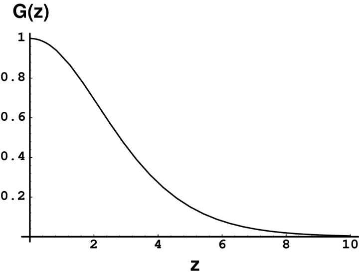
Figure 4.3: The scale function $G(z)$ for the open and flat Universes.

4.3.2 The Einstein Universe

In the case of the closed universe, the spatial mode functions are the four-dimensional spherical harmonics, which have the form [66, 14]

$$[\epsilon=1]:\qquad\quad U_{\lambda}({\bf x}) = (2\omega_{n}a^{3})^{-1/2}\,\Pi^{(+)}_{nl}(\chi)\,{\rm Y}_{lm}(\theta,\varphi)\,,$$ (4.71)

$$\omega_{n} = \sqrt{{n(n+2)\over a^{2}}+\mu^{2}},$$ (4.72)

$$\lambda = (n,l,m).$$

Here, $n=0,1,2,\cdots;\quad l=0,1,\cdots,n;$ and $m=-l,-l+1,\cdots,+l$. The function $\Pi^{(+)}$ is found from $\Pi^{(-)}$ by replacing $\chi$ by $-i\chi$ and $q$ by $-i(n+1)$ [66]. Alternatively, they can be written in terms of Gegenbauer polynomials [14, 69] as

$$\Pi^{(+)}_{nl}(\chi)\propto\sin^{l}\chi\;{\rm C}^{l+1}_{n-l}(\cos\chi).$$ (4.73)

In either case, the addition theorem is found from Eq. 11.4(3) of [69] (with $p=2$ and $\xi=\eta$). This reduces to

$$\sum_{lm}|\Pi^{(+)}_{nl}(\chi){\rm Y}_{lm}(\theta,\varphi)|^{2}={(n+1)^{2}\over 2\pi^{2}}\,,$$ (4.74)

from which it is easy to show that the energy density inequality, Eq. (3.18), becomes

$$\Delta\hat{\rho}\geq-{1\over 4\pi^{2}a^{3}}\sum_{n=0}^{\infty}(n+1)^{2}\,\omega_{n}\,{\rm e}^{-2\omega_{n}t_{0}}.$$ (4.75)

If we use the variable $\eta={t_{0}/a}$ in the above equation, we can simplify it to

$$\Delta\hat{\rho}\geq-{3\over 32\pi^{2}t_{0}^{4}}H(\eta,\mu).$$ (4.76)

Again we find the flat space solution in four dimensions, multiplied by the scale function $H(\eta,\mu)$, which is defined as

$$H(\eta,\mu)\equiv{8\over 3}\eta^{4}\sum_{n=1}^{\infty}(n+1)^{2}\sqrt{n(n+2)+a^{2}\mu^{2}}\;{\rm e}^{-2\eta\sqrt{n(n+2)+a^{2}\mu^{2}}},$$ (4.77)

and is plotted in Figure 4.4 for $\mu=0$. The scale function here has a small bump occurring at roughly $\eta\approx 0.5$ with a height of 1.03245. This may permit the magnitude of the negative energy to be slightly greater for a massless scalar field in the Einstein universe than is allowed in a flat universe for comparable sampling times. A similar result was shown to exist for massive fields in two-dimensional Minkowski spacetime [48].

4.3.3 Massless Asymptotic Limits in the Einstein Universe

As with the three-dimensional closed universe, we can find the asymptotic limits of this function. We again follow the method of the previous section, assuming the scalar field is massless, and making use of the Plana summation formula to find

$$H(\eta,0)={8\over 3}\eta^{4}\,\bigl{(}I_{2}+I_{3}\bigr{)}\,,$$ (4.78)

where

$$I_{2}=\int_{0}^{\infty}(x+1)^{2}\sqrt{x(x+2)}\,{\rm e}^{-2\eta\sqrt{x(x+2)}}\,dx\,,$$ (4.79)

and

$$I_{3} = 2{\rm Re}\left[i\int_{0}^{\infty}{(ix+1)^{2}\sqrt{ix(ix+2)}{\rm e}^{-2\eta\sqrt{ix(ix+2)}}\over{\rm e}^{2\pi x}-1}\,dx\right],$$ (4.80)

$$= \int_{0}^{\infty}\sqrt{2x}\>\frac{(x^{2}-1)\sqrt{\sqrt{x^{2}+4}+x}-2x\sqrt{\sqrt{x^{2}+4}-x}}{{\rm e}^{2\pi x}-1}\>{\rm d}x\,,$$

$$\approx -0.356109\,.$$

The first integral can be done in terms of Struve ${\bf H}_{n}(z)$ and Neumann $N_{n}(z)$ functions, with the result

$$I_{2}={\pi\over 16}{d^{2}\over d\eta^{2}}\left[{1\over\eta}\left({\bf H}_{1}(2\eta)-N_{1}(2\eta)\right)\right]+\frac{4}{15}\eta\,.$$ (4.81)

If we follow the same procedure as in the previous section for defining the renormalized vacuum energy density for the minimally coupled scalar field in the Einstein universe, then we obtain

$$\rho_{Casimir}={1\over{4\pi^{2}a^{4}}}\,I_{3}\approx-{0.356109\over{4\pi^{2}a^{4}}}\,.$$ (4.82)

The same method yields $\rho_{Casimir}=1/{480\pi^{2}a^{4}}$ for the massless conformal scalar field [13]. Here our result for the minimal field, Eq. (4.82), differs from that obtained by Elizalde [15] using the zeta function method, $\rho^{\prime}_{Casimir}=-0.411502/{4\pi^{2}a^{4}}$. This discrepancy probably reflects that the renormalized vacuum energy density is not uniquely defined. The renormalized stress-tensor in a curved spacetime is only defined up to additional finite renormalizations of the form of those required to remove the infinities. In general this includes the geometrical tensors ${}^{(1)}H_{\mu\nu}$ and ${}^{(2)}H_{\mu\nu}$. (See any of the references in [53, 55, 70] for the definitions of these tensors and a discussion of their role in renormalization.) In the Einstein universe, both of these tensors are nonzero and are proportional to $1/a^{4}$. Thus the addition of these tensors to $\langle T_{\mu\nu}\rangle$ will change the numerical coefficient in $\rho_{Casimir}$. The logarithmically divergent parts of $\langle T_{\mu\nu}\rangle$ which are proportional to ${}^{(1)}H_{\mu\nu}$ and ${}^{(2)}H_{\mu\nu}$ happen to vanish in the Einstein universe, but not in a more general spacetime. In principle, we should imagine that the renormalization procedure is performed in an arbitrary spacetime, and only later do we specialize to a specific metric. Unfortunately, it is computationally impossible to do this explicitly. Thus, the fact that a particular divergent term happens to vanish in a particular spacetime does not preclude the presence of finite terms of the same form.

In the small $\eta$ limit, we can expand the Struve and the Neumann functions in Eq. (4.81) in a Taylor series to obtain

$$H(\eta,0)=1+{1\over 3}\eta^{2}+{(3+4\gamma)\over 12}\eta^{4}+{8\over 3}(-0.356109)\eta^{4}+{1\over 3}\eta^{4}\ln\eta+O(\eta^{6})+\cdots,$$ (4.83)

where $\gamma$ is Euler’s constant, which arises in the Taylor series expansion of the Neumann function. This is similar to that of the three-dimensional universe and again contains a term of the form of the Casimir energy. In the large $\eta$ limit we again keep just the first term of the series (4.77). Both asymptotic forms are plotted with the exact solution in Figure 4.4. We see that the asymptotic form is again a very good approximation except in the interval $1<\eta<2$, as was the case for the three-dimensional closed universe.

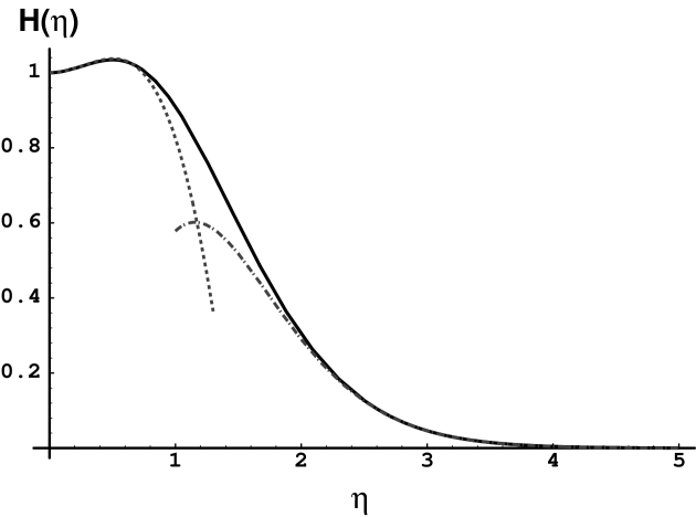
Figure 4.4: The scale function $H(\eta)$ for the Einstein universe. The solid line is the exact result. The dotted line is the asymptotic expansion for small $\eta$, while the dot-dash curve is the large $\eta$ approximation. The maximum occurs at $\eta\approx 0.5$.

The difference inequalities for massless fields are then given by

$$\Delta\hat{\rho}\geq-{3\over{32\pi^{2}t_{0}^{4}}}\left[1+{1\over 3}\eta^{2}+{(3+4\gamma)\over 12}\eta^{4}+{1\over 3}\eta^{4}\ln\eta+\cdots\right]-\rho_{Casimir}\,,$$ (4.84)

for $t_{0}\ll a$ and

$$\Delta\hat{\rho}\geq-{\sqrt{3}\over{\pi^{2}a^{4}}}\,{\rm e}^{-2\sqrt{3}\,t_{0}/a},\qquad{\rm for}\quad t_{0}\gg a\,.$$ (4.85)

Using $\Delta\hat{\rho}=\hat{\rho}_{Ren.}-\hat{\rho}_{Casimir}$, where $\hat{\rho}_{Casimir}$ is the expectation value of $\rho_{Ren.}$ in the vacuum state, we can calculate the renormalized energy density that would be constrained by the quantum inequalities, subject to renormalization ambiguities. For example, in the four-dimensional Einstein universe the renormalized energy density inequality is

$$\hat{\rho}_{Ren.}\geq-{3\over{32\pi^{2}t_{0}^{4}}}\left[1+{1\over 3}\eta^{2}+{(3+4\gamma)\over 12}\eta^{4}+{1\over 3}\eta^{4}\ln\eta+O(\eta^{6})+\cdots\right]\,,$$ (4.86)

for $t_{0}\ll a$. Here the coefficient of the $\eta^{4}$ term could be altered by a finite renormalization, but the rest of the expression is unambiguous. This result is identical to the short sampling time expansion of the quantum inequality in the Einstein universe, Eq. (3.59), developed in Section 3.3. Expressions similar to Eq. (4.86) could be found for any of the other cases above. In the case of the flat Robertson-Walker universe, there is no Casimir vacuum energy. Under such circumstances the difference inequality and the renormalized energy density inequality are the same, and are free of ambiguities.

4.4 Quantum Inequalities Near Planar Mirrors

4.4.1 Single Mirror

Consider four-dimensional Minkowski spacetime with a perfectly reflecting boundary at $z=0$, located in the $x-y$ plane, at which we require the scalar field to vanish. The two-point function can be found by using the standard Feynman Green’s function in Minkowski space,

$$G^{(0)}_{F}(x,x^{\prime})={-i\over 4\pi^{2}[(x-x^{\prime})^{2}+(y-y^{\prime})^{2}+(z-z^{\prime})^{2}-(t-t^{\prime})^{2}]},$$ (4.87)

and applying the method of images to find the required Green’s function when the boundary is present. For a single conducting plate we have

$$G_{F}(x,x^{\prime}) = {-i\over 4\pi^{2}}\left[{1\over{(x-x^{\prime})^{2}+(y-y^{\prime})^{2}+(z-z^{\prime})^{2}-(t-t^{\prime})^{2}}}\right.$$ (4.88)

$$\qquad-\left.{1\over{(x-x^{\prime})^{2}+(y-y^{\prime})^{2}+(z+z^{\prime})^{2}-(t-t^{\prime})^{2}}}\right].$$

If we Euclideanize by allowing $t\rightarrow-it_{0}$, $t^{\prime}\rightarrow it_{0}$ and then take $x^{\prime}\rightarrow x$, we find

$$G_{E}(2t_{0})={1\over 16\pi^{2}}\left({1\over t_{0}^{2}}-{1\over{t_{0}^{2}+z^{2}}}\right).$$ (4.89)

In addition, the Euclidean box operator is given by

$$\mathord{\hbox{\Bxfnt\char 116\relax}\hbox to0.0pt{\hss\Bxfnt\char 117\relax}}_{E}=\partial^{2}_{t_{0}}+\partial^{2}_{x}+\partial^{2}_{y}+\partial^{2}_{z}.$$ (4.90)

It is easily shown that the quantum inequality is given by

$$\Delta\hat{\rho}\geq-{1\over 4}\,\mathord{\hbox{\Bxfnt\char 116\relax}\hbox to0.0pt{\hss\Bxfnt\char 117\relax}}_{E}\,G_{E}(2t_{0})=-{3\over 32\pi^{2}\,t_{0}^{4}}+{1\over 16\pi^{2}(t_{0}^{2}+z^{2})^{2}}\,.$$ (4.91)

The first term of this inequality is identical to that for Minkowski space. The second term represents the effect of the mirror on the quantum inequality. For the minimally coupled scalar field we know from Eq. (2.66) that there is a non-zero, negative vacuum energy density which diverges as the mirror is approached. Adding this vacuum term to both the left- and right-hand sides of the above expression allows us to find the renormalized quantum inequality for this spacetime,

$$\hat{\rho}_{Ren.}\geq-{3\over 32\pi^{2}\,t_{0}^{4}}+{1\over 16\pi^{2}(t_{0}^{2}+z^{2})^{2}}-{1\over 16\pi^{2}z^{4}}\,.$$ (4.92)

There are two limits in which the behavior of the renormalized quantum inequality can be studied. First consider $z\gg t_{0}$. In this limit, the correction term due to the mirror, and the vacuum energy very nearly cancel and the quantum inequality reduces to

$$\hat{\rho}_{Ren.}\geq-{3\over 32\pi^{2}\,t_{0}^{4}}\,.$$ (4.93)

This is exactly the expression for the quantum inequality in Minkowski spacetime. Thus, if an observer samples the energy density on time scales which are small compared to the light travel time to the boundary, then the Minkowski space quantum inequality is a good approximation.

The other important limit is when $z\ll t_{0}$. This is the case for observations made very close to the mirror, but for very long times. The quantum inequality then reduces to

$$\hat{\rho}_{Ren.}\geq-{1\over 16\pi^{2}\,z^{4}}\,.$$ (4.94)

Here, we see that the quantum field is satisfying the quantum averaged weak energy condition. Recall that throughout the present paper, we are concerned with observers at rest with respect to the plate. If the observer is moving and passes through the plate, then it is necessary to reformulate the quantum inequalities in terms of sampling functions with compact support [71]. It should be noted that the divergence of the vacuum energy on the plate is due to the unphysical nature of perfectly reflecting boundary conditions. If the mirror becomes transparent at high frequencies, the divergence is removed. Even if the mirror is perfectly reflecting, but has a nonzero position uncertainty, the divergence is also removed [72].

4.4.2 Two Parallel Plates

Now let us consider the case of two parallel plates, one located in the $z=0$ plane and another located in the $z=L$ plane. We are interested in finding the quantum inequality in the region between the two plates, namely $0\leq z\leq L$. We can again use the method of images to find the Green’s function. In this case, not only do we have to consider the reflection of the source in each mirror, but we must also take into account the reflection of one image in the other mirror, and then the reflection of the reflections. This leads to an infinite number of terms that must be summed to find the exact form of the Green’s function. If we place a source at $(t^{\prime},x^{\prime},y^{\prime},z^{\prime})$, then there is an image of the source at $(t^{\prime},x^{\prime},y^{\prime},-z^{\prime})$ from the mirror at $z=0$ and a second image at $(t^{\prime},x^{\prime},y^{\prime},2L-z^{\prime})$ from the mirror at $z=L$. Then, we must add the images of these images to the Green’s function, continuing ad infinitum for every pair of resulting images. If we use the notation

$$G_{F}(z,a\pm z^{\prime})\equiv G^{(0)}_{F}(t,x,y,z;t^{\prime},x^{\prime},y^{\prime},a\pm z^{\prime}),$$ (4.95)

where $a$ is a constant, then we can write the Green’s functions between the plates as

$$G(x,x^{\prime}) = G_{F}(z,z^{\prime})-G_{F}(z,-z^{\prime})+\sum_{n=1}^{\infty}\left[G_{F}(z,2nL+z^{\prime})-G_{F}(z,-2nL-z^{\prime})\right.$$ (4.96)

$$\left.+G_{F}(z,-2nL+z^{\prime})-G_{F}(z,2nL-z^{\prime})\right].$$

We Euclideanize as above, and let the spatial separation between the source and observer points go to zero, to find

$$G_{E}(2t_{0}) = {1\over 16\pi^{2}}\left({1\over t_{0}^{2}}-{1\over{t_{0}^{2}+z^{2}}}\right)$$ (4.97)

$$\qquad+{1\over 16\pi^{2}}\sum_{n=1}^{\infty}\left[{2\over{t_{0}^{2}+(nL)^{2}}}-{1\over{t_{0}^{2}+(nL+z)^{2}}}-{1\over{t_{0}^{2}+(nl-z)^{2}}}\right].$$

It is now straightforward to find the quantum inequality,

$$\Delta\hat{\rho} \geq -{3\over 32\pi^{2}\,t_{0}^{4}}\,+{1\over 16\pi^{2}(t_{0}^{2}+z^{2})^{2}}$$ (4.98)

$$\qquad+{1\over 16\pi^{2}}\sum_{n=1}^{\infty}\left\{{(nL)^{2}-3t_{0}^{2}\over[t_{0}^{2}+(nL)^{2}]^{3}}+{1\over[t_{0}^{2}+(nL+z)^{2}]^{2}}+{1\over[t_{0}^{2}+(nL-z)^{2}]^{2}}\right\}.$$

The first term in the expression above is identical to that found for Minkowski space. The second term is the modification of the quantum inequality due to the mirror at $z=0$. The modification due to the presence of the second mirror is contained in the summation, as well as all of the multiple reflection contributions. When the Casimir vacuum energy, given by [55]

$$\rho_{vacuum}=-{\pi^{2}\over 48L^{4}}\,{3-2\sin^{2}(\pi z/L)\over\sin^{4}(\pi z/L)}\,-\,{\pi^{2}\over 1440L^{4}}\,,$$ (4.99)

is added back into this equation for renormalization, we find, as with a single mirror, that close to the mirror surfaces the vacuum energy comes to dominate and the quantum inequality becomes extremely weak.

4.5 Spacetimes with Horizons

We will now change from flat spacetimes with boundaries to spacetimes in which there exist horizons. We will begin with the two-dimensional Rindler spacetime to develop the quantum inequality for uniformly accelerating observers. For these observers, there exists a particle horizon along the null rays $x=\pm t$ (see Figure 4.5).

We will then look at the static coordinatization of de Sitter spacetime. Again there exists a particle horizon in this spacetime, somewhat similar to that of the Rindler spacetime. The two problems differ because Rindler spacetime is flat while the de Sitter spacetime has constant, positive spacetime curvature.

4.5.1 Two-Dimensional Rindler Spacetime

We begin with the usual two-dimensional Minkowski metric

$$ds^{2}=-dt^{2}+dx^{2}.$$ (4.100)

Now let us consider an observer who is moving with constant acceleration. We can transform to the observer’s rest frame (Section 4.5 of [53]) by

$$t = a^{-1}e^{a\xi}\sinh a\eta\,,$$ (4.101)

$$x = a^{-1}e^{a\xi}\cosh a\eta\,,$$ (4.102)

where $a$ is a constant related to the acceleration by

$$a\;e^{-a\xi}={\rm proper\ acceleration}.$$ (4.103)

The metric in the rest frame of the observer is then given by

$$ds^{2}=e^{2a\xi}(-d\eta^{2}+d\xi^{2}).$$ (4.104)

The accelerating observer’s coordinates $(\eta,\xi)$ only cover one quadrant of Minkowski spacetime, where $x>|t|$. This is shown in Figure 4.5. Four different coordinate patches are required to cover all of Minkowski spacetime in the regions labeled L, R, F, and P. For the remainder of the paper we will be working specifically in the left and right regions, labeled L and R respectively. In these two regions, uniformly accelerating observers in Minkowski spacetime can be represented by observers at rest at constant $\xi$ in Rindler coordinates, as shown by the hyperbola in Figure 4.5.

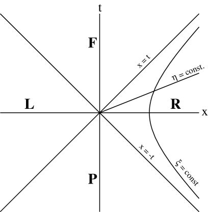
Figure 4.5: The Rindler coordinatization of two-dimensional Minkowski spacetime. The time coordinate $\eta=$ constant are straight lines passing through the origin, while the space coordinate $\xi=$ constant are hyperbolæ. The Minkowski spacetime is covered by four separate coordinate patches, labeled by L, R, F, and P. The two null rays ($x=t$ and $x=-t$) act as horizons.

The massless scalar wave equation in Rindler spacetime is given by

$$e^{-2a\xi}\left(-{d^{2}\over d\eta^{2}}+{d^{2}\over d\xi^{2}}\right)\phi(\eta,\xi)=0,$$ (4.105)

which has the positive frequency mode function solutions

$$f_{k}(\eta,\xi)=(4\pi\omega)^{-1/2}\;e^{ik\xi\pm i\omega\eta}.$$ (4.106)

Here $-\infty<k<\infty$ and $\omega=|k|$. The plus and minus signs correspond to the left and right Rindler wedges, respectively. Using the above mode functions, we can expand the general solution as

$$\phi(\eta,\xi)=\int_{-\infty}^{\infty}dk\left[b_{k}^{L}f_{k}(\eta,\xi)+{b_{k}^{L}}^{\dagger}f_{k}^{*}(\eta,\xi)+b_{k}^{R}f_{k}(\eta,\xi)+{b_{k}^{R}}^{\dagger}f_{k}^{*}(\eta,\xi)\right],$$ (4.107)

where ${b_{k}^{L}}^{\dagger}$ and ${b_{k}^{L}}$ are the creation and annihilation operators in the left Rindler wedge and similarly for ${b_{k}^{R}}^{\dagger}$ and ${b_{k}^{R}}$ in the right Rindler wedge. We also need to define two vacua, $|0_{L}\rangle$ and $|0_{R}\rangle$, with the properties

$${b_{k}^{L}}^{\dagger}|0_{R}\rangle={b_{k}^{R}}^{\dagger}|0_{L}\rangle=b_{k}^{L}|0_{L}\rangle=b_{k}^{L}|0_{R}\rangle=b_{k}^{R}|0_{L}\rangle=b_{k}^{L}|0_{R}\rangle=0.$$ (4.108)

The Rindler particle states are then excitations above the vacuum given by

$$|\{1_{k}\}_{L}\rangle = {b_{k}^{L}}^{\dagger}|0_{L}\rangle,$$ (4.109)

$$|\{1_{k}\}_{R}\rangle = {b_{k}^{R}}^{\dagger}|0_{R}\rangle.$$ (4.110)

With this in hand, we can find the two-point function in either the left or right regions. Let us consider the right Rindler wedge, where

$$G^{+}(x,x^{\prime}) = \langle 0_{R}|\phi(x)\phi(x^{\prime})|0_{R}\rangle,$$ (4.111)

$$= \int_{-\infty}^{\infty}dk\,f_{k}(x)f_{k}^{*}(x^{\prime})\,,$$

$$= {1\over 4\pi}\int_{-\infty}^{\infty}{dk\over\omega}e^{ik(\xi-\xi^{\prime})-i\omega(\eta-\eta^{\prime})}.$$

To find the Euclidean two-point function required for the quantum inequality, we first allow the spatial separation to go to zero and then take $(\eta-\eta^{\prime})\rightarrow-2i\eta_{0}$, yielding

$$G_{E}(2\eta_{0})={1\over 2\pi}\int_{0}^{\infty}{d\omega\over\omega}e^{-2\omega\eta_{0}}.$$ (4.112)

In two dimensions, the Euclidean Green’s function for the massless scalar field has an infrared divergence as can be seen from the form above, in which the integral is not well defined in the limit of $\omega\rightarrow 0$. However, in the process of finding the quantum inequality we act on the Green’s function with the Euclidean box operator. If we first take the derivatives of the Green’s function, and then carry out the integration, the result is well defined for all values of $\omega$. In Rindler space, the Euclidean box operator is given by

$$\mathord{\hbox{\Bxfnt\char 116\relax}\hbox to0.0pt{\hss\Bxfnt\char 117\relax}}_{E}=e^{-2a\xi}\left({d^{2}\over d\eta^{2}}+{d^{2}\over d\xi^{2}}\right).$$ (4.113)

It is now easy to solve for the quantum inequality

$$\Delta\hat{\rho}\geq-{1\over 4}\mathord{\hbox{\Bxfnt\char 116\relax}\hbox to0.0pt{\hss\Bxfnt\char 117\relax}}_{E}G_{E}(2\eta_{0})=-{1\over 2\pi}e^{-2a\xi}\int_{o}^{\infty}d\omega\;\omega e^{-2\omega\eta_{0}}=-{1\over 8\pi\left(e^{a\xi}\,\eta_{0}\right)^{2}}\,.$$ (4.114)

However, the coordinate time $\eta_{0}$ is related to the observer’s proper time by

$$\tau_{0}=e^{a\xi}\eta_{0}\,,$$ (4.115)

allowing us to rewrite the quantum inequality in a more covariant form,

$$\Delta\hat{\rho}\geq-{1\over 8\pi\tau_{0}^{2}}\,.$$ (4.116)

This is exactly the same form of the quantum inequality as found in two-dimensional Minkowski spacetime [32, 48]. As we have seen in Section 4.1.1, this is a typical property of static two-dimensional spacetimes which arises because all two-dimensional static spacetimes are conformal to one another. However, we reiterate that the renormalized quantum inequalities are not identical in different spacetimes because of differences in the vacuum energies.

4.5.2 de Sitter Spacetime

Let us now consider four-dimensional de Sitter spacetime. The scalar field quantum inequality, Eq. (3.23), assumes a timelike Killing vector, so it will be convenient to use the static parametrization of de Sitter space,

$$ds^{2}=-(1-{r^{2}\over\alpha^{2}})\,dt^{2}+(1-{r^{2}\over\alpha^{2}})^{-1}dr^{2}+r^{2}(d\theta^{2}+\sin^{2}\theta\;d\varphi^{2})\;.$$ (4.117)

There is a particle horizon at $r=\alpha$ for an observer sitting at rest at $r=0$. The coordinates take the values, $0\leq r<\alpha$, $0\leq\theta\leq\pi$, and $0\leq\varphi<2\pi$. It should be noted that this choice of metric covers one quarter of de Sitter spacetime.

The scalar wave equation is

$$\left(1-{r^{2}\over\alpha^{2}}\right)^{-1}\partial_{t}^{2}\phi-{1\over r^{2}}\partial_{r}\left[r^{2}\left(1-{r^{2}\over\alpha^{2}}\right)\partial_{r}\right]\phi-{{\bf L}^{2}\over r^{2}}\phi+\mu^{2}\phi=0\,,$$ (4.118)

where ${\bf L}^{2}$ is the square of the standard angular momentum operator and is defined by

$${\bf L}^{2}={1\over\sin\theta}\partial_{\theta}\left(\sin\theta\,\partial_{\theta}\right)+{1\over\sin^{2}\theta}\partial_{\varphi}^{2}\,.$$ (4.119)

The unit norm positive frequency mode functions are found [73, 74, 75, 76, 77] to be of the form

$$\hat{\phi}_{\omega,l,m}(t,r,\theta,\varphi)={1\over\sqrt{4\pi\alpha^{3}\omega}}\;f_{\omega}^{l}(z)\;{\rm Y}_{lm}(\theta,\varphi)\;e^{-i\omega t},$$ (4.120)

where $z=r/\alpha$ is a dimensionless length, ${\rm Y}_{lm}(\theta,\varphi)$ are the standard spherical harmonics, and the mode labels $l$ and $m$ take the values $l=0,1,2,\cdots$ and $-l\leq m\leq l$. The radial portion of the the solution is given by

$$f_{\omega}^{l}(z)={\Gamma(b^{+}_{l})\Gamma(b^{-}_{l})\over\Gamma(l+{3\over 2})\Gamma(i\alpha\omega)}\;z^{l}\;(1-{z^{2}})^{i\alpha\omega/2}\;{\rm F}(\,b^{-}_{l},\,b^{+}_{l};\,l+{3\over 2};\,z^{2})\,,$$ (4.121)

where ${\rm F}(\alpha,\beta;\gamma;z)$ is the hypergeometric function [78] and

$$b^{\pm}_{l}={1\over 2}\left(l+{3\over 2}+i\alpha\omega\pm\sqrt{{9\over 4}-\alpha^{2}\mu^{2}}\right).$$ (4.122)

We can then express the two-point function as

$$G(x,x^{\prime})=\sum_{lm}\int_{0}^{\infty}\,dk{1\over 4\pi\alpha^{2}k}{f_{k}^{l}}^{*}(z)\;f_{k}^{l}(z^{\prime})\;{\rm Y}_{lm}^{*}(\theta,\varphi)\;{\rm Y}_{lm}(\theta^{\prime},\varphi^{\prime})\;e^{ik(t-t^{\prime})/a},$$ (4.123)

where $k\equiv\alpha\omega$. Now if we Euclideanize according to Eq. (3.21) and set the spatial separation of the points to zero, we may use the addition theorem for the spherical harmonics, Eq. (4.36), to find the Euclidean Green’s function

$$G_{E}={1\over 16\pi^{2}\alpha^{2}}\sum_{l}\int_{0}^{\infty}dk{(2l+1)\over k}\left|{\Gamma(b^{+}_{l})\Gamma(b^{-}_{l})\over\Gamma(l+{3\over 2})\Gamma(ik)}\right|^{2}z^{2l}\,\left|{\rm F}(b^{-}_{l},b^{+}_{l};l+{3\over 2};\,z^{2})\right|^{2}e^{-2kt_{0}/\alpha}\,.$$ (4.124)

This is independent of the angular coordinates, as expected, because de Sitter spacetime is isotropic. We now need the Euclidean box operator. Because of the angular independence of the Green’s function, it is only necessary to know the temporal and radial portions of the box operator. The energy density inequality, Eq. (3.23), then becomes

$$\Delta\hat{\rho}\geq-{1\over 4}\left\{{1\over(1-z^{2})}\partial_{t_{0}}^{2}+{1\over\alpha^{2}z^{2}}\partial_{z}\left[z^{2}\,(1-z^{2})\partial_{z}\right]\right\}\;G_{E}({\bf x},-t_{0};{\bf x},+t_{0}).$$ (4.125)

The temporal derivative term in Eq. (4.125) will simply bring down two powers of $k/\alpha$. Using the properties of the hypergeometric function, it can be shown that

$$\left|{\rm F}(b^{-}_{l},b^{+}_{l};l+{3\over 2};\,z^{2})\right|^{2}=(1-z^{2})^{ik}\;{\rm F}^{2}(b^{-}_{l},b^{+}_{l};l+{3\over 2};\,z^{2}),$$ (4.126)

from which we can take the appropriate spatial derivatives. If we allow $z\rightarrow 0$, then we have $F\rightarrow 1$ and only the $l=0$ terms will contribute in the time derivative part of Eq. (4.125). For the radial derivative, it is possible to show that

$$\lim_{z\rightarrow 0}{1\over z^{2}}\partial_{z}\left\{z^{2}\,(1-z^{2})\partial_{z}\left[z^{2l}(1-z^{2})^{ik}{\rm F}^{2}(z^{2})\right]\right\}=\left\{\matrix{2(\alpha^{2}\mu^{2}-k^{2})&{\rm for}\;l=0,\cr 6&{\rm for}\;l=1,\cr 0&{\rm otherwise.}}\right.$$ (4.127)

Using this result, we find for the observer at $r=0$ that

$$\Delta\hat{\rho}\geq-{1\over 8\pi^{4}\alpha^{4}}\int_{0}^{\infty}dk\sinh(\pi k)\left[(k^{2}+\alpha^{2}\mu^{2})\left|\Gamma(b^{-}_{0})\Gamma(b^{+}_{0})\right|^{2}+4\left|\Gamma(b^{-}_{1})\Gamma(b^{+}_{1})\right|^{2}\right]e^{-2t_{0}k/\alpha}.$$ (4.128)

There are two cases for which the right-hand side can be evaluated analytically, $\mu=0$ and $\mu=\sqrt{2}/\alpha$. For $\mu=0$, we have

$$\Delta\hat{\rho} \geq -{1\over 8\pi^{4}\alpha^{4}}\int_{0}^{\infty}dk\sinh(\pi k)\left[k^{2}\left|\Gamma(i{k\over 2})\,\Gamma({3\over 2}+i{k\over 2})\right|^{2}+4\left|\Gamma({1\over 2}+i{k\over 2})\,\Gamma(2+i{k\over 2})\right|^{2}\right]e^{-2t_{0}k/\alpha},$$ (4.129)

$$= -{1\over 8\pi^{2}\alpha^{4}}\int_{0}^{\infty}dk(2k^{3}+5k)e^{-2t_{0}k/\alpha}=-{3\over 32\pi^{2}t_{0}^{4}}\left[1+{5\over 3}\left({t_{0}\over\alpha}\right)^{2}\right]\,,$$

where we have used the identities for gamma functions proven in Appendix B. Similarly for $\mu=\sqrt{2}/\alpha$, we find

$$\Delta\hat{\rho}\geq-{3\over 32\pi^{2}t_{0}^{4}}\left[1+\left({t_{0}\over\alpha}\right)^{2}\right].$$ (4.130)

We can compare these results with the short sampling time approximation from Section 3.3. Solving for the necessary geometrical coefficients, we find

$$v_{000} = \left({29\over 60}{1\over\alpha^{4}}-{1\over 4}{\mu^{2}\over\alpha^{2}}\right)|g_{tt}|\,,$$ (4.131)

$$v_{1} = {29\over 60}{1\over\alpha^{4}}-{1\over 2}{\mu^{2}\over\alpha^{2}}+{1\over 8}\mu^{4}\,,$$ (4.132)

$${1\over 2}g_{tt}\nabla^{j}\nabla_{j}\,g_{tt}^{-1} = {1\over\alpha^{2}}{\left(3-r^{2}/\alpha^{2}\right)\over\left(1-r^{2}/\alpha^{2}\right)}\,.$$ (4.133)

The general short sampling time expansion, Eq. (LABEL:eq:QI_expansion), now becomes

$$\Delta\hat{\rho} \geq -{3\over 32\pi^{2}\tau_{0}^{4}}\left\{1+{1\over 3}\left[{2\over\alpha^{2}}-\mu^{2}+{1\over\alpha^{2}}{(3-r^{2}/\alpha^{2})\over(1-r^{2}/\alpha^{2})}\right]\,\tau_{0}^{2}\right.$$ (4.134)

$$\qquad\qquad\left.+{\mu^{2}\over 6}\left(\mu^{2}-{2\over\alpha^{2}}\right)\,\tau_{0}^{4}\,\ln(2\tau_{0}^{2}/\alpha^{2})+O(\tau_{0}^{4})+\cdots\right\},$$

where $\tau_{0}=(1-r^{2}/\alpha^{2})^{1/2}t_{0}$. If $r=0$ and $\mu$ takes the values $0$ or $\sqrt{2}/\alpha$, this agrees with Eqs. (4.129) or (4.130), respectively. Note that this small $t_{0}$ expansion is valid for all radii, $0\leq r<\alpha$. We can also find the proper sampling time from Eq. (3.56) for which this expansion is valid,

$$\tau_{0}\ll\tau_{m}\equiv\alpha\sqrt{{1-r^{2}/\alpha^{2}}\over{5-3r^{2}/\alpha^{2}}}.$$ (4.135)

For the observer sitting at the origin of the coordinate system, $\tau_{0}\ll\alpha/\sqrt{5}$. This is the scale on which the spacetime can be considered “locally flat.” For observers at $r>0$, who do not move on geodesics, $\tau_{m}$ decreases and approaches zero as $r\rightarrow\alpha$:

$$\tau_{m}\sim\sqrt{\alpha(\alpha-r)},\qquad r\rightarrow\alpha.$$ (4.136)

Note that the proper distance to the horizon from radius $r$ is

$$\ell=\int_{r}^{\alpha}{dr^{\prime}\over\sqrt{1-r^{\prime 2}/\alpha^{2}}}=\alpha\left[\pi/2-\arcsin(r/\alpha)\right]\sim\sqrt{2\alpha(\alpha-r)},\qquad\mbox{ as }r\rightarrow\alpha.$$ (4.137)

Thus, for observers close to the horizon, if the sampling time is small compared to this distance to the horizon, i.e., if $\tau_{0}\ll\ell$, then $\tau_{0}\ll\tau_{m}$ and the short sampling time expansion is valid.

We can also obtain a renormalized quantum inequality for the energy density at the origin for the case $\mu=\sqrt{2}\alpha$. By the addition of the vacuum energy to both sides of Eq. (4.130) we find for $r=0$

$$\hat{\rho}_{Ren.}\geq-{3\over 32\pi^{2}t_{0}^{4}}\left[1+\left({t_{0}\over\alpha}\right)^{2}\right]-{1\over 960\pi^{2}\alpha^{4}}\,.$$ (4.138)

We can now predict what will happen in the infinite sampling time limit of the renormalized quantum inequality for any observer’s position. We know from Eqs. (4.124) and (4.125) that the difference inequality will always go to zero, yielding a QAWEC in static de Sitter spacetime of

$$\lim_{t_{0}\rightarrow\infty}{t_{0}\over\pi}\int_{-\infty}^{\infty}{\langle T_{tt}u^{0}u^{0}\rangle_{Ren.}\over t^{2}+t_{0}^{2}}dt\geq{1\over 480\pi^{2}\alpha^{4}}\left[-{\alpha^{2}\over(\alpha^{2}-r^{2})}+{1\over 2}(1-{r^{2}\over\alpha^{2}})\right].$$ (4.139)

We immediately see that for a static observer who is arbitrarily close to the horizon in de Sitter spacetime, the right hand side of Eq. (4.139) becomes extremely negative, and diverges on the horizon itself. This is similar to the behavior found for static observers located near the perfectly reflecting mirror discussed earlier and for Rindler space.

4.6 Black Holes

We now turn our attention to an especially interesting spacetime in which quantum inequalities can be developed, the exterior region of a black hole in two and four dimensions.

4.6.1 Two-Dimensional Black Holes

Let us consider the metric

$$ds^{2}=-C(r)\,dt^{2}+C(r)^{-1}\,dr^{2}\,,$$ (4.140)

where $C(r)$ is a function chosen such that $C\rightarrow 1$ and $\partial C/\partial r\rightarrow 0$ as $r\rightarrow\infty$. Additionally, there is an event horizon at some value $r_{0}$ where $C(r_{0})=0$. For example, in the Schwarzschild spacetime, $C(r)=1-2Mr^{-1}$, there is a horizon at $r=2M$. Another choice for $C$ is that of the Reissner-Nordström black hole, where $C(r)=1-2Mr^{-1}+Q^{2}r^{-2}$. In general, we will leave the function $C$ unspecified for the remainder of the derivation. The above metric leads to the massless, minimally coupled scalar wave equation

$$-{1\over C(r)}\partial_{t}^{2}\phi(r,t)+\partial_{r}\left[C(r)\partial_{r}\phi(r,t)\right]=0\,.$$ (4.141)

Unlike in four dimensions, the two-dimensional wave equation can be analytically solved everywhere. If we use the standard definition of the $r^{*}$ coordinate,

$$r^{*}\equiv\int{dr\over C(r)}\,,$$ (4.142)

then it is convenient for us to take as the definition of the positive frequency mode functions

$$f_{k}(r,t)=i\left(4\pi\omega\right)^{-1/2}\;e^{ikr^{*}-i\omega t},\qquad\omega=|k|,$$ (4.143)

where $-\infty<k<\infty$.

The problem of finding the quantum inequality simply reduces to using the mode functions to find the Euclidean Green’s function. We have

$$G_{E}(2t_{0})=\int_{-\infty}^{\infty}dk\;\left|{i\over\sqrt{4\pi\omega}}e^{ikr^{*}}\right|^{2}\,e^{-2\omega t_{0}}={1\over 2\pi}\int_{0}^{\infty}d\omega\;\omega^{-1}e^{-2\omega t_{0}}.$$ (4.144)

As in the case of two-dimensional Rindler space, the Euclidean Green’s function has an infrared divergence. We can again apply the Euclidean box operator first and then do the integration to obtain the quantum inequality,

$$\Delta\hat{\rho}\geq-{1\over 2\pi C(r)}\int_{0}^{\infty}d\omega\;\omega\,e^{-2\omega t_{0}}=-{1\over 8\pi C(r)t_{0}^{2}}\,.$$ (4.145)

However, the observer’s proper time is related to the coordinate time by $\tau=C(r)^{1/2}t$, such that we can write the difference inequality as

$$\Delta\hat{\rho}\geq-{1\over 8\pi\tau_{0}^{2}}.$$ (4.146)

This is the same form as found for two-dimensional Minkowski and Rindler spacetimes. This is the expected result because of the conformal equivalence of all two-dimensional spacetimes.

This now brings us to the matter of renormalization. There exist three candidates for the vacuum state of a black hole: the Boulware vacuum, the Hartle-Hawking vacuum, and the Unruh vacuum. However the derivation of the difference inequality relies on the mode functions being defined to have positive frequency with respect to the timelike Killing vector $\partial_{t}$, and the vacuum state being destroyed by the annihilation operator, i.e.,

$$a_{k}\;|0_{k}\rangle=0,\qquad\mbox{for all }k\,.$$ (4.147)

In Schwarzschild spacetime, this defines the Boulware vacuum. Thus, we can solve for the renormalized quantum inequality,

$$\hat{\rho}_{Ren.}\equiv{t_{0}\over\pi}\int_{-\infty}^{\infty}{\langle{T_{tt}/|g_{tt}|}\rangle_{Ren.}\over{t^{2}+t_{0}^{2}}}dt\geq-{1\over 8\pi\tau_{0}^{2}}+\rho_{B}(r)\;.$$ (4.148)

The Boulware vacuum energy density in two dimensions for the Reissner-Nordström black hole is given explicitly by (see Section 8.2 of [53])

$$\rho_{B}(r)={1\over 24\pi}\left(1-{2M\over r}+{Q^{2}\over r^{2}}\right)^{-1}\left[-{4M\over r^{3}}+{7M^{2}\over r^{4}}+{6Q^{2}\over r^{4}}-{14MQ^{2}\over r^{5}}+{5Q^{4}\over r^{6}}\right].$$ (4.149)

In the limit $\tau_{0}\rightarrow\infty$, we recover a QAWEC condition on the energy density

$$\lim_{t_{0}\rightarrow\infty}{t_{0}\over\pi}\int_{-\infty}^{\infty}{\langle{T_{tt}/g_{tt}}\rangle_{Ren.}\over t^{2}+t_{0}^{2}}dt\geq\rho_{B}(r).$$ (4.150)

This has the interpretation that the integrated energy density in an arbitrary particle state can never be more negative than that of the Boulware vacuum state. In particular, this will be true for the Hartle-Hawking and Unruh vacuum states.

4.6.2 Four-Dimensional Schwarzschild Spacetime

Now let us turn to the four-dimensional Schwarzschild spacetime with the metric

$$ds^{2}=-\left(1-{2M\over r}\right)dt^{2}+\left(1-{2M\over r}\right)^{-1}dr^{2}+r^{2}\,(d\theta^{2}+\sin^{2}\theta\,d\varphi^{2})\,.$$ (4.151)

The normalized mode functions for a massless scalar field in the exterior region ($r>2M$) of Schwarzschild spacetime can be written as [54]

$$\stackrel{{\scriptstyle\rightarrow}}{{f}}_{\omega lm}(x) = (4\pi\omega)^{1/2}e^{-i\omega t}\stackrel{{\scriptstyle\rightarrow}}{{R}}_{l}(\omega|r){\rm Y}_{lm}(\theta,\varphi),$$

$$\stackrel{{\scriptstyle\leftarrow}}{{f}}_{\omega lm}(x) = (4\pi\omega)^{1/2}e^{-i\omega t}\stackrel{{\scriptstyle\leftarrow}}{{R}}_{l}(\omega|r){\rm Y}_{lm}(\theta,\varphi),$$ (4.152)

where $\stackrel{{\scriptstyle\rightarrow}}{{R}}_{l}(\omega|r)$ and $\stackrel{{\scriptstyle\leftarrow}}{{R}}_{l}(\omega|r)$ are the outgoing and ingoing solutions to the radial portion of the wave equation, respectively. Although they cannot be written down analytically, their asymptotic forms are

$$\stackrel{{\scriptstyle\rightarrow}}{{R}}_{l}(\omega|r)\sim\left\{\begin{array}[]{ll}r^{-1}e^{i\omega r^{*}}+\stackrel{{\scriptstyle\rightarrow}}{{\rm A}}_{l}(\omega)r^{-1}e^{-i\omega r^{*}}\,,&\qquad r\rightarrow 2M,\\ {\rm B}_{l}(\omega)r^{-1}e^{i\omega r^{*}}\,,&\qquad r\rightarrow\infty,\end{array}\right.$$ (4.153)

for the outgoing modes and

$$\stackrel{{\scriptstyle\leftarrow}}{{R}}_{l}(\omega|r)\sim\left\{\begin{array}[]{ll}{\rm B}_{l}(\omega)r^{-1}e^{-i\omega r^{*}}\,,&\qquad r\rightarrow 2M,\\ r^{-1}e^{-i\omega r^{*}}+\stackrel{{\scriptstyle\leftarrow}}{{\rm A}}_{l}(\omega)r^{-1}e^{i\omega r^{*}}\,,&\qquad r\rightarrow\infty,\end{array}\right.$$ (4.154)

for the ingoing modes. The normalization factors ${\rm B}_{l}(\omega)$, $\stackrel{{\scriptstyle\rightarrow}}{{\rm A}}_{l}(\omega)$, and $\stackrel{{\scriptstyle\leftarrow}}{{\rm A}}_{l}(\omega)$ are the transmission and reflection coefficients for the scalar field with an angular momentum-dependent potential barrier.

Now let us consider the two-point function in the Boulware vacuum. It is given by

$$G_{B}(x,x^{\prime})=\sum_{lm}\int_{0}^{\infty}{d\omega\over 4\pi\omega}e^{-i\omega(t-t^{\prime})}\,{\rm Y}_{lm}(\theta,\varphi){\rm Y}_{lm}^{*}(\theta^{\prime},\varphi^{\prime})\,\left[\stackrel{{\scriptstyle\rightarrow}}{{R}}_{l}(\omega|r)\stackrel{{\scriptstyle\rightarrow}}{{R}}_{l}^{*}(\omega|r^{\prime})+\stackrel{{\scriptstyle\leftarrow}}{{R}}_{l}(\omega|r)\stackrel{{\scriptstyle\leftarrow}}{{R}}_{l}^{*}(\omega|r^{\prime})\right]\,.$$ (4.155)

We are interested in the two-point function when the spatial separation goes to zero, i.e., letting $r^{\prime}\rightarrow r$, $\theta^{\prime}\rightarrow\theta$, and $\varphi^{\prime}\rightarrow\varphi$. We can again make use of the addition theorem for the spherical harmonics, Eq. (4.36). Let us also Euclideanize, by taking $(t-t^{\prime})\rightarrow-2it_{0}$. The Euclidean two-point function then reduces to

$$G_{BE}(2t_{0})={1\over 16\pi^{2}}\sum_{l}\int_{0}^{\infty}{d\omega\over\omega}\,e^{-2t_{0}}\,(2l+1)\,\left[|\stackrel{{\scriptstyle\rightarrow}}{{R}}_{l}(\omega|r)|^{2}+|\stackrel{{\scriptstyle\leftarrow}}{{R}}_{l}(\omega|r)|^{2}\right]\,.$$ (4.156)

In the two asymptotic regimes, close to the event horizon of the black hole ($r\rightarrow 2M$), or far from the black hole ($r\rightarrow\infty$), the radial portion of the wave equation also satisfies a sum rule. It was found by Candelas [79] that

$$\sum_{l=0}^{\infty}(2l+1)|\stackrel{{\scriptstyle\rightarrow}}{{R}}_{l}(\omega|r)|^{2}\sim\left\{\begin{array}[]{ll}4\omega^{2}(1-2M/r)^{-1},&\qquad r\rightarrow 2M,\\ r^{-2}\sum_{l=0}^{\infty}(2l+1)|{\rm B}_{l}(\omega)|^{2},&\qquad r\rightarrow\infty,\end{array}\right.$$ (4.157)

and

$$\sum_{l=0}^{\infty}(2l+1)|\stackrel{{\scriptstyle\leftarrow}}{{R}}_{l}(\omega|r)|^{2}\sim\left\{\begin{array}[]{ll}(2M)^{-2}\sum_{l=0}^{\infty}(2l+1)|{\rm B}_{l}(\omega)|^{2},&\qquad r\rightarrow 2M,\\ 4\omega^{2},&\qquad r\rightarrow\infty,\end{array}\right.$$ (4.158)

with the coefficient ${\rm B}_{l}(\omega)$ given, in the case $2M\omega\ll 1$, by [80]

$${\rm B}_{l}(\omega)\approx{(l!)^{3}\over(2l+1)!\,(2l)!}\,(-4iM\omega)^{l+1}\,.$$ (4.159)

If we insert these relations into the Green’s functions, it is possible to carry out the integration in $\omega$. In the near field limit

$$G_{BE}(2t_{0})\sim{1\over 16\pi^{2}}\left[{1\over(1-2M/r)t_{0}^{2}}+{1\over 4M^{2}}\sum_{l=0}{(l!)^{6}\over[(2l)!]^{3}}\,\left({2M\over t_{0}}\right)^{2l+2}\right],\qquad r\rightarrow 2M,$$ (4.160)

and in the far field limit,

$$G_{BE}(2t_{0})\sim{1\over 16\pi^{2}}\left[{1\over t_{0}^{2}}+{1\over r^{2}}\sum_{l=0}{(l!)^{6}\over[(2l)!]^{3}}\,\left({2M\over t_{0}}\right)^{2l+2}\right],\qquad r\rightarrow\infty.$$ (4.161)

We immediately see that the Green’s function is independent of the angular coordinates, as expected from the spherical symmetry. Note that the maximum value of $l$ for which the expansion in Eqs. (4.160) and (4.161) can be used depends upon the order of the leading terms which have been dropped in Eq. (4.159). If this correction is $O\left((M\omega)^{l+2}\right)$, then only the $l=0$ terms are significant, as $B_{0}$ would then contain subdominant pieces which yield a contribution to $G_{BE}(2t_{0})$ larger than the leading contribution from $B_{1}$. In what follows, we will explicitly retain only the $l=0$ contribution. In order to find the quantum inequality around a black hole we must evaluate

$$\Delta\hat{\rho}\geq-{1\over 4}\,\mathord{\hbox{\Bxfnt\char 116\relax}\hbox to0.0pt{\hss\Bxfnt\char 117\relax}}_{E}\;G_{E}(2t_{0}).$$ (4.162)

However, the only parts of the Euclidean box operator that are relevant are the temporal and radial terms, i.e.,

$$\mathord{\hbox{\Bxfnt\char 116\relax}\hbox to0.0pt{\hss\Bxfnt\char 117\relax}}_{E}\Rightarrow(1-{2M/r})^{-1}\partial_{t_{0}}^{2}+r^{-2}\partial_{r}[r^{2}(1-{2M/r})\partial_{r}].$$ (4.163)

Upon taking the appropriate derivatives, and using the relation of the proper time of a stationary observer to the coordinate time,

$$\tau_{0}=t_{0}\,\sqrt{1-{2M/r}}\,,$$ (4.164)

we find that the quantum inequality is given by

$$\Delta\hat{\rho}\geq-{3\over 32\pi^{2}\tau_{0}^{4}}\left\{{1\over 6}\left(2M\over r\right)^{2}\left(\tau_{0}\over r\right)^{2}\left(1-{2M\over r}\right)^{-1}+1+\left(1-{2M\over r}\right)+O\left[\left(1-{2M\over r}\right)^{2}\right]+\cdots\right\},$$ (4.165)

as $r\rightarrow 2M$ and

$$\Delta\hat{\rho} \geq -{3\over 32\pi^{2}\tau_{0}^{4}}\left\{1-{2M\over r}+\left({2M\over r}\right)^{2}\left[1+{1\over 3}\left({\tau_{0}\over r}\right)^{2}\right]\right.$$ (4.166)

$$\qquad\qquad\left.-\left({2M\over r}\right)^{3}\left[1+\left({\tau_{0}\over r}\right)^{2}\right]+O\left[\left({2M\over r}\right)^{4}\right]+\cdots\right\},$$

as $r\rightarrow\infty$. An alternative approach to finding the quantum inequality is to use the short time expansion from Section 3.3, which yields

$$\Delta\hat{\rho}\geq-{3\over 32\pi^{2}\tau_{0}^{4}}-{1\over 16\pi^{2}\tau_{0}^{2}}\left[{M^{2}\over r^{4}(1-2M/r)}+O(\tau_{0}^{2})+\cdots\right].$$ (4.167)

Note that this short time expansion coincides with the first two terms of the $r\rightarrow 2M$ form, Eq. (4.165). This is somewhat unexpected, as Eq. (4.165) is an expansion for small $r-2M$ with $\tau_{0}$ fixed, whereas Eq. (4.167) is an expansion for small $\tau_{0}$ with $r$ fixed.

We immediately see from Eq. (4.166) that we recover the Minkowski space quantum inequality in the $r\rightarrow\infty$ limit. If we consider experiments performed on the surface of the earth, where the radius of the earth is several orders of magnitude larger than its equivalent Schwarzschild radius, then the flat space inequality is an exceptionally good approximation. From Eq. (3.56), we can also find the proper sampling time for which the inequality Eq. (4.167) holds,

$$\tau_{0}\ll{r^{2}\over 2M}\sqrt{2\left(1-{2M\over r}\right)}.$$ (4.168)

As was the case in two dimensions, if we allow the sampling time to go to infinity in the exact quantum inequality, we recover the QAWEC, Eq. (4.150), for the four-dimensional black hole. The QAWEC says that the renormalized energy density for an arbitrary particle state, sampled over the entirety of the rest observer’s worldline, can never be more negative than the Boulware vacuum energy density.

Chapter 5 A Dynamic Spacetime: The Warp Drive

In the preceding chapters, we looked at various static spacetimes in which quantum inequalities could be developed. Now we will apply the quantum inequality restrictions for a scalar field to Alcubierre’s warp drive metric on a scale in which a local region of spacetime can be considered “flat.” This is accomplished by taking the sampling time of the quantum inequality to be very small. Over short timescales, the equivalence principle tells us that the spacetime should be nearly static and almost flat. The short sampling time expansion of the quantum inequality developed in Section 3.3 tells us that on short enough time scales we can apply the Minkowski space quantum inequality with reasonable reliability. From this we are able to place limits on the parameters of the “warp bubble.” We will show that the bubble wall thickness is on the order of only a few hundred Planck lengths. Additionally, we will show that the total integrated energy density needed to maintain the warp metric with such thin walls is physically unattainable.

5.1 Introduction

In both the scientific community and pop culture, humans have been fascinated with the prospect of being able to travel between the stars within their own lifetimes. Within the framework of special relativity, the space-going traveler may move with any velocity up to, but not including, the speed of light. The astronauts would experience a time dilation which would allow them to make the round trip from earth to any star, and back to earth, in an arbitrarily short elapsed time. However, upon returning to earth such observers would find that their family and friends would have aged considerably. This is the well-known twin paradox [1, 81, 82].

Recently, Miguel Alcubierre proposed a metric [39], fondly called the warp drive, in which a spaceship could travel to a star a distance $D$ away and return home, such that the elapsed time for the stationary observers on earth would be less than $2D/c$, where $c$ is the velocity of light. What is most surprising about this spacetime is that the proper time of the space going traveler’s trip is identical to the elapsed time on earth. However, the spaceship never locally travels faster than the speed of light. In fact, the spaceship can sit at rest with respect to the interior of the warp bubble. The ship is carried along by the spacetime, much in the same way that the galaxies are receding away from each other at extreme speeds due to the expansion of the universe, while locally they are at rest. The warp drive utilizes this type of expansion and contraction in order to achieve the ability to travel faster than light.

Although warp drive sounds appealing, it does have one serious drawback. As with traversable wormholes, in order to achieve warp drive we must employ exotic matter, that is, negative energy densities, which are a violation of the classical energy conditions. We have seen that the quantum inequality restrictions do allow negative energy densities to exist [16, 32, 45, 47, 48]. However, they place serious limitations on their magnitude and duration. Even before the short sampling time expansion of the quantum inequality was developed, researchers had applied the flat space quantum inequality to the curved spacetime geometries of wormholes [44] with the restriction that the negative energy be sampled on timescales smaller than the minimum local radius of curvature. It was argued that over such small sampling times, the spacetime would be locally flat and the inequalities would be valid. This led to the conclusion that static wormholes must either be on the order of several Planck lengths in size, or there would be large discrepancies in the length scales that characterize the wormhole.

As we have seen in the preceding chapter, exact quantum inequalities can be developed for the static spacetimes in two, three, and four dimensions [35]. It was found that the quantum inequalities take the flat space form modified by a scale function which depends on the sampling time, the local radius of curvature, and the mass of the scalar field. In the limit of the sampling time being smaller than the local radius of curvature, the quantum inequalities reduce to the flat space form, often accompanied by higher order corrections due to the curvature [35, 36]. In the limit of the radius of curvature going to infinity, the flat space inequalities are recovered.

We would like to apply the same method to the warp drive metric, but such an exercise would require that we know the solutions to the Klein-Gordon equation for the mode functions of the scalar field. Such an approach, although exact, would be exceptionally difficult. In this section we will therefore apply the flat space inequality directly to the warp drive metric but restrict the sampling time to be small. We will thereby be able to show that the walls of the warp bubble must be exceedingly thin compared to its radius. This constrains the negative energy to an exceedingly thin band surrounding the spaceship. Similar results have been demonstrated for wormholes [44], where the negative energy is concentrated in a thin band around the throat. Recently, it has been shown for the Krasnikov metric [41], which also allows superluminal travel, that the required negative energy is also constrained to a very thin wall [42]. We will then calculate the total negative energy that would be required to generate a macroscopic sized bubble capable of transporting humans. As we will see, such a bubble would require physically unattainable energies.

5.2 Warp Drive Basics

Let us discuss some of the basic principles of the warp drive spacetime. We begin with a flat (Minkowski) spacetime and then consider a small spherical region, which we will call the bubble, inside this spacetime. On the forward edge of the bubble, we cause spacetime to contract, and on the trailing edge is an equal spacetime expansion. The region inside the bubble, which can be flat, is therefore transported forward with respect to distant objects. Objects at rest inside the bubble are transported forward with the bubble, even though they have no (or nominal) local velocity. Such a spacetime is described by the Alcubierre warp drive metric

$$ds^{2}=-dt^{2}+[dx-v_{s}(t)f(r_{s}(t))dt]^{2}+dy^{2}+dz^{2},$$ (5.1)

where $x_{s}(t)$ is the trajectory of the center of the bubble and $v_{x}(t)=dx_{s}(t)/{dt}$ is the bubble’s velocity. The variable $r_{s}(t)$ measures the distance outward from the center of the bubble given by

$$r_{s}(t)=\sqrt{(x-x_{s}(t))^{2}+y^{2}+z^{2}}.$$ (5.2)

The shape function of the bubble is given by $f(r_{s})$, which Alcubierre originally chose to be

$$f(r_{s})={{\tanh[\sigma(r_{s}-R)]-\tanh[\sigma(r_{s}+R)]}\over 2\tanh[\sigma\;R]}.$$ (5.3)

The variable $R$ is the radius of the warp bubble, and $\sigma$ is a free parameter which can be used to describe the thickness of the bubble walls. In the large $\sigma$ limit, the function $f(r_{s})$ quickly approaches that of a top hat function, where $f(r_{s})=1$ for $r_{s}\leq R$ and zero everywhere else. It is not necessary to choose a particular form of $f(r_{s})$. Any function will suffice so long as it has the value of approximately 1 inside some region $r_{s}<R$ and goes to zero rapidly outside the bubble, such that as $r_{s}\rightarrow\infty$ we recover Minkowski space. In order to make later calculations easier, we will use the piecewise continuous function

$$f_{p.c.}(r_{s})=\left\{\begin{array}[]{ll}1&r_{s}<R-{\Delta\over 2},\\ -{1\over\Delta}(r_{s}-R-{\Delta\over 2})&R-{\Delta\over 2}<r_{s}<R+{\Delta\over 2},\\ 0&r_{s}>R+{\Delta\over 2},\end{array}\right.$$ (5.4)

where $R$ is the radius of the bubble. The variable $\Delta$ is the bubble wall thickness. It is chosen to relate to the parameter $\sigma$ for the Alcubierre form of the shape function by setting the slopes of the functions $f(r_{s})$ and $f_{p.c.}(r_{s})$ to be equal at $r_{s}=R$. This leads to

$$\Delta={\left[1+\tanh^{2}(\sigma R)\right]^{2}\over 2\;\sigma\;\tanh(\sigma R)}\;,$$ (5.5)

which in the limit of large $\sigma R$ can be approximated by $\Delta\simeq 2/\sigma$.

We now turn our attention to the solutions of the geodesic equation. It is straightforward to show that

$${dx^{\mu}\over dt}=u^{\mu}=\left(1,v_{s}(t)f(r_{s}(t)),0,0\right),\qquad u_{\mu}=(-1,0,0,0),$$ (5.6)

is a first integral of the geodesic equations. Observers with this four-velocity are called the Eulerian observers by Alcubierre. We see that the proper time and the coordinate time are the same for all observers. Also, the y and z components of the four-velocity are zero. The bubble therefore exerts no “force” in the directions perpendicular to the direction of travel. In Figure 5.1, we have plotted one such trajectory for a observer that passes through the wall of a warp bubble at a distance $\rho$ away from the center of the bubble. The x-component of the four-velocity is dependent on the shape function, and solving this explicitly for all cases can be rather difficult due to the time dependence of $r_{s}(t)$. A spacetime plot of an observer with the four-velocity given above is shown in Figure 5.2 for a bubble with constant velocity.

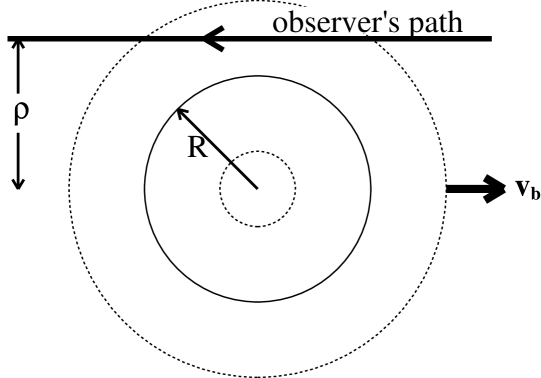
Figure 5.1: The path of an observer who passes through the outer region of the bubble, shown in the bubble’s rest frame. As viewed from the interior of the bubble, the observer is moving to the left.

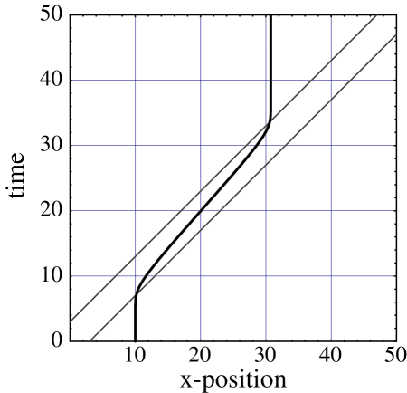
Figure 5.2: The worldline (the dark line) of the geodesic observer passing through the outer region of a warp bubble, plotted in the observer’s initial rest frame. The two lighter diagonal lines are the worldlines of the center of the bubble wall on the front and rear edges of the bubble, respectively. The bubble has a radius of 3, a velocity of 1, and a $\sigma$ of 1. The plot shows an observer who begins at rest at $x=10$, $y^{2}+z^{2}=\rho^{2}=4$. The shape function is of the form given by Alcubierre, Eq. (5.3).

We see that the Eulerian observers are initially at rest. As the front wall of the bubble approaches, the observer begins to accelerate in the direction of travel of the bubble, relative to observers at large distances. Once inside the bubble the observer moves with a nearly constant velocity given by

$$\left.{dx(t)\over dt}\right|_{max.}=v_{s}(t_{\rho})f(\rho),$$ (5.7)

which will always be less than the bubble’s velocity unless $\rho=(y^{2}+z^{2})^{1/2}=0$. The time $t_{\rho}$ is defined by $r_{s}(t_{\rho})=\rho$, i.e., it is the time at which the observer reaches the bubble equator. Such observers then decelerate, and are left at rest as they pass from the rear edge of the bubble wall. In other words no residual momentum is imparted to these observers during the “collision.” However, they have been displaced forward in space along the trajectory of the bubble.

There is also another interesting feature of these geodesics. As already noted, the observers will move with a nearly constant velocity through the interior of the bubble. This holds true for any value of $\rho$. However, the velocity is still dependent upon the value of $\rho$, so observers at different distances from the center of the bubble will be moving with different velocities relative to one another. If a spaceship of finite size is placed inside the bubble with its center of mass coincident with the center of the bubble, then the ship will experience a net “force” pushing it opposite to the direction of motion of the bubble so long as $1-f(r_{s})$ is nonzero at the walls of the ship. The ship would therefore have to use its engines to maintain its position inside the bubble. In addition, the ship would be subject to internal stresses on any parts that extended sufficiently far away from the center of the bubble

In the above discussion we have used the Alcubierre form of the shape function, $f(r_{s})$. If the piecewise continuous form, Eq. (5.4), is used, one finds similar results with some modification. Inside the bubble, where $r_{s}<(R-{\Delta/2})$, every observer would move at exactly the speed of the bubble. So any observer who reached the bubble interior would continue on with it forever. This arises because everywhere inside the bubble, spacetime is perfectly flat due to $f(r_{s})=1$. For observers whose geodesics pass solely through the bubble walls, so $(R-{\Delta/2})<\rho<(R+{\Delta/2})$, the result is more or less identical to that of the geodesics found with the Alcubierre shape function. This is the most interesting region because it contains the largest magnitude of negative energy.

We now turn our attention to the energy density distribution of the warp drive metric. Using the first integral of the geodesic equations, it is easily shown that

$$\langle T^{\mu\nu}u_{\mu}u_{\nu}\rangle=\langle T^{tt}\rangle={1\over 8\pi}G^{tt}=-{1\over 8\pi}{v_{s}^{2}(t)\rho^{2}\over 4r_{s}^{2}(t)}\left(df(r_{s})\over dr_{s}\right)^{2},$$ (5.8)

where $\rho=[y^{2}+z^{2}]^{1/2}$, is the radial distance perpendicular to the $x$-axis defined above. We immediately see that the energy density measured by any Eulerian observer is always negative, as shown in Alcubierre’s original paper [39]. In Figure 5.3, we see that the distribution of negative energy is concentrated in a toroidal region perpendicular to the direction of travel.

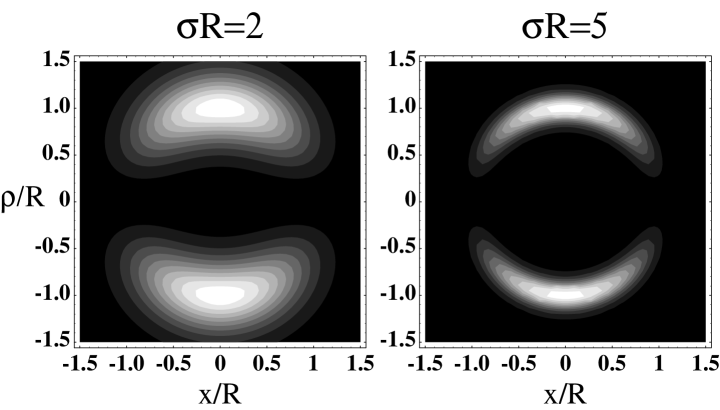
Figure 5.3: The negative energy density is plotted for a longitudinal cross section of the warp metric traveling at constant velocity $v_{s}=1$ to the right for the Alcubierre shape function. Black regions are devoid of matter, while white regions are maximal negative energy.

In Section 5.4 we will integrate the energy density over all of space to obtain the total negative energy required to maintain the bubble, under the restrictions of the quantum inequalities. As we will show, the total energy is physically unrealizable in the most extreme sense.

5.3 Quantum Inequality Restrictions

We begin with the quantum inequality (QI) for a free, massless scalar field in four-dimensional Minkowski spacetime originally derived by Ford and Roman [32],

$${\tau_{0}\over\pi}\int_{-\infty}^{\infty}{{\langle T_{\mu\nu}u^{\mu}u^{\nu}\rangle}\over{\tau^{2}+\tau_{0}^{2}}}d\tau\geq-{3\over{32\pi^{2}\tau_{0}^{4}}}\;,$$ (5.9)

where $\tau$ is an inertial observer’s proper time, and $\tau_{0}$ is an arbitrary sampling time. It has been argued by Ford and Roman [44] that one may apply the QI to non-Minkowski spacetimes if the sampling time is smaller than the local radius of curvature. We know this to be true. It comes from the small sampling time expansion of the QI developed in Section 3.3.

We begin by taking the expression for the energy density (5.8), and inserting it into the quantum inequality, Eq. (5.9), yielding

$$t_{0}\int_{-\infty}^{+\infty}{v_{s}(t)^{2}\over r_{s}^{2}}\left({df(r_{s})\over dr_{s}}\right)^{2}{dt\over{t^{2}+t_{0}^{2}}}\leq{3\over\rho^{2}t_{0}^{4}}\,.$$ (5.10)

If the time scale of the sampling is sufficiently small compared to the time scale over which the bubble’s velocity is changing, then the warp bubble’s velocity can be considered roughly constant, $v_{s}(t)\approx v_{b}$, during the sampling interval. We can now find the form of the geodesic at the time the sampling is taking place. Because of the small sampling time, the $[t^{2}+t_{0}^{2}]^{-1}$ term becomes strongly peaked, causing the QI integral to sample only a small portion of the geodesic. We therefore place the observer at the equator of the warp bubble at $t=0$. Then the geodesic is well-approximated by

$$x(t)\approx f(\rho)v_{b}t\;,$$ (5.11)

which results in

$$r_{s}(t)=\left[(v_{b}t)^{2}(f(\rho)-1)^{2}+\rho^{2}\right]^{1/2}\;.$$ (5.12)

Finally, we must specify the form of the shape function of the bubble. We can expand any shape function as a Taylor series about the sampling point, $r_{s}(t)\rightarrow\rho$. Then we take the appropriate derivatives to obtain the term needed for the quantum inequality. We find

$${df(r_{s})\over dr_{s}}\approx f^{\prime}(\rho)+f^{\prime\prime}(\rho)[r_{s}(t)-\rho]+\cdots.$$ (5.13)

The leading term is the slope of the shape function at the sampling point, which is in general roughly proportional to the inverse of the bubble wall thickness. We can therefore use, with no loss of generality, the piecewise continuous form of the shape function (5.4) to obtain a good order of magnitude approximation for any choice of shape function. The quantum inequality (5.10) then becomes

$$t_{0}\int_{-\infty}^{+\infty}{dt\over(t^{2}+\beta^{2})(t^{2}+t_{0}^{2})}\leq{3\Delta^{2}\over v_{b}^{2}\,t_{0}^{4}\,\beta^{2}},$$ (5.14)

where

$$\beta={\rho\over{v_{b}(1-f(\rho))}}\,.$$ (5.15)

Formally the integral should not be taken over all time but just the time the observer is inside the bubble walls. However, the sampling function rapidly approaches zero. Therefore contributions to the integral from the distant past or the far future are negligible. The integral itself can be performed as the principal value of a contour that is closed in the upper half of the complex plane,

$$\int_{-\infty}^{+\infty}{dt\over(t^{2}+\beta^{2})(t^{2}+t_{0}^{2})}={\pi\over t_{0}\;\beta\;(t_{0}+\beta)},$$ (5.16)

yielding an inequality of

$${\pi\over 3}\leq{\Delta^{2}\over{v_{b}^{2}\;t_{0}^{4}}}\left[{v_{b}t_{0}\over\rho}(1-f(\rho))+1\right]\;.$$ (5.17)

The above inequality is valid only for sampling times on which the spacetime may be considered approximately flat. We must therefore find some characteristic length scale below which this occurs. For an observer passing through the bubble wall at a distance $\rho$ from the center, the Riemann tensor in the static background frame can be calculated. Then we transform the components to the observer’s frame by use of an orthonormal tetrad of unit vectors. In this frame, the tetrad is given by the velocity vector $u^{\mu}(t)$ and three unit vectors $\hat{x}$, $\hat{y}$, and $\hat{z}$. The largest component of the Riemann tensor in the orthonormal frame is given by

$$|R_{{\hat{t}}{\hat{y}}{\hat{t}}{\hat{y}}}|={3v_{b}^{2}\;y^{2}\over 4\;\rho^{2}}\left[{df(\rho)\over d\rho}\right]^{2}.$$ (5.18)

This yields

$$r_{min}\equiv{1\over\sqrt{|R_{{\hat{t}}{\hat{y}}{\hat{t}}{\hat{y}}}|}}\sim{2\Delta\over{\sqrt{3}}\;v_{b}}\;,$$ (5.19)

when $y=\rho$ and the piecewise continuous form of the shape function is used. The sampling time must be smaller than this length scale, so we take

$$t_{0}=\alpha{2\Delta\over{\sqrt{3}}\;v_{b}},\qquad 0<\alpha\ll 1.$$ (5.20)

Here $\alpha$ is the ratio of the sampling time to the minimal radius of curvature. If we insert this into the quantum inequality and use

$${\Delta\over\rho}\sim{v_{b}t_{0}\over\rho}\ll 1\;,$$ (5.21)

we may neglect the term involving $1-f(\rho)$ to find

$$\Delta\leq{3\over 4}\sqrt{3\over\pi}\;{v_{b}\over\alpha^{2}}\,.$$ (5.22)

Now as an example, if we let $\alpha=1/10$, then

$$\Delta\leq 10^{2}\,v_{b}\;L_{Planck}\,,$$ (5.23)

where $L_{Planck}$ is the Planck length. Thus, unless $v_{b}$ is extremely large, the wall thickness cannot be much above the Planck scale. Typically, the walls of the warp bubble are so thin that the shape function could be considered a “step function” for most purposes.

5.4 Total Energy Calculation

We will now look at the total amount of negative energy that is involved in the maintenance of a warp metric. For simplicity, let us take a bubble that moves with constant velocity such that $x_{s}(t)=v_{b}\,t$. Because the total energy is constant, we can calculate it at time $t=0$. We then have

$$r_{s}(t=0)=[x^{2}+y^{2}+z^{2}]^{1\over 2}=r.$$ (5.24)

With this in mind we can write the integral of the local matter energy density over proper volume as

$$E=\int dx^{3}\sqrt{|g|}\;\,\langle T^{tt}\rangle=-{v_{b}^{2}\over 32\pi}\int{\rho^{2}\over r^{2}}\left(df(r)\over dr\right)^{2}dx^{3}\;,$$ (5.25)

where $g={\rm Det}|g_{ij}|$ is the determinant of the spatial metric on the constant time hypersurfaces. Portions of this integration can be carried out by making a transformation to spherical coordinates. By doing so, we find

$$E=-{1\over 12}v_{b}^{2}\int_{0}^{\infty}r^{2}\left(d\;f(r)\over dr\right)^{2}dr\,.$$ (5.26)

Since we are making only order of magnitude estimates of the total energy, we will use a piecewise continuous approximation to the shape function given by Eq. (5.4). Taking the derivative of this shape function, we find that the contributions to the energy come only from the bubble wall region, and we end up evaluating

$$E = -{1\over 12}v_{b}^{2}\int_{R-{\Delta\over 2}}^{R+{\Delta\over 2}}r^{2}\left(-1\over\Delta\right)^{2}dr,$$ (5.27)

$$= -{1\over 12}v_{b}^{2}\left({R^{2}\over\Delta}+{\Delta\over 12}\right).$$

For a macroscopically useful warp drive, we want the radius of the bubble to be at least in the range of 100 meters so that we may fit a ship inside. We showed in the previous section that the wall thickness is constrained by (5.23). If we use this constraint and let the bubble radius be equal to 100 meters, then we may neglect the second term on the right-hand-side of Eq. (5.27). It follows that

$$E\leq-6.2\times 10^{70}\,v_{b}\;L_{Planck}\;\sim\;-6.2\times 10^{65}\,v_{b}\;{\rm grams}.$$ (5.28)

Because a typical galaxy has a mass of approximately

$$M_{MilkyWay}\approx 10^{12}\;M_{sun}=2\times 10^{45}{\rm grams},$$ (5.29)

the energy required for a warp bubble is on the order of

$$E\leq-3\times 10^{20}\;M_{galaxy}\;v_{b}\;.$$ (5.30)

This is a fantastic amount of negative energy, roughly ten orders of magnitude greater than the total mass of the entire visible universe.

If it were possible to violate the quantum inequality restrictions and make a bubble with a wall thickness on the order of a meter, things would be somewhat improved. The total energy required in the case of the same size radius and $\Delta=1$ meter would be on the order of a quarter of a solar mass, which would be more practical, yet still not attainable.

5.5 Summary

We see from Eq. (5.23), that quantum inequality restrictions on the warp drive metric constrain the bubble walls to be exceptionally thin. Typically, the walls are on the order of only hundreds or thousands of Planck lengths. Similar constraints on the size of the negative energy region have been found in the case of traversable wormholes [44].

From Eq. (5.23), we may think that by making the velocity of the bubble very large we can make the walls thicker. However, this causes another problem. For every order of magnitude by which the velocity increases, the total negative energy required to generate the warp drive metric also increases by the same magnitude. It is evident that for macroscopically sized bubbles to be useful for human transportation, even at subluminal speeds, the required negative energy is physically unattainable.

On the other hand, we may consider the opposite regime. Warp bubbles are still conceivable if they are very tiny, i.e., much less than the size of an atom. Here the difference in length scales is not as great. As a result, a smaller amount of negative energy is required to maintain the warp bubble. For example, a bubble with a radius of one electron Compton wavelength would require a negative energy of order $E\sim-400M_{sun}$.

The above derivation assumes that we are using a quantized, massless scalar field to generate the required negative energy. Similar quantum inequalities have been proven for both massive scalar fields [35, 48] and the electromagnetic field [48]. In the case of the massive scalar field, the quantum inequality becomes even more restrictive, thereby requiring the bubble walls to be even thinner. For the quantized electromagnetic field, the wall thickness can be made larger by a factor of $\sqrt{2}$, due to the two spin degrees of freedom of the photon. However this is not much of an improvement over the scalar field case.

Appendix A Inequalities

In this appendix, we prove the following inequality: Let $A_{ij}$ be a real, symmetric $n\times n$ matrix with non-negative eigenvalues. (For the purposes of this manuscript, we may take either $n=2$, for three-dimensional spacetimes, or $n=3$, for four-dimensional spacetimes.) Further let $h_{\lambda}^{i}$ be a complex $n$-vector, which is also a function of the mode label $\lambda$. Then in an arbitrary quantum state $|\psi\rangle$, the inequality states that

$${\rm Re}\sum_{\lambda,\lambda^{\prime}}A_{ij}\left[h^{i\,*}_{\lambda}h^{j}_{\lambda^{\prime}}\langle a_{\lambda}^{\dagger}a_{\lambda^{\prime}}\rangle\pm h^{i}_{\lambda}h^{j}_{\lambda^{\prime}}\langle a_{\lambda}a_{\lambda^{\prime}}\rangle\right]\geq-{1\over 2}\sum_{\lambda}A_{ij}h^{i\,*}_{\lambda}h^{j}_{\lambda}\,.$$ (A.1)

In order to prove this relation, we first note that

$$A_{ij}=\sum_{\alpha=1}^{n}\kappa_{\alpha}V_{i}^{(\alpha)}\,V_{j}^{(\alpha)}\,,$$ (A.2)

where the $V_{i}^{(\alpha)}$ are the eigenvectors of $A_{ij}$, and the $\kappa_{\alpha}\geq 0$ are the corresponding eigenvalues. Now define the hermitian vector operator

$$Q^{i}=\sum_{\lambda}\left(h^{i\,*}_{\lambda}a_{\lambda}^{\dagger}+h^{i}_{\lambda}a_{\lambda}\right)\,.$$ (A.3)

Note that

$$\left\langle{Q^{i}}^{\dagger}A_{ij}Q^{j}\right\rangle=\sum_{\alpha=1}^{n}\kappa_{\alpha}\left\langle Q^{i\,\dagger}V_{i}^{(\alpha)}\,V_{j}^{(\alpha)}Q^{j}\right\rangle=\sum_{\alpha=1}^{n}\kappa_{\alpha}||V_{i}^{(\alpha)}\,Q^{i}|\psi\rangle||^{2}\geq 0\,.$$ (A.4)

Furthermore,

$$\left\langle Q^{i\,\dagger}A_{ij}Q^{j}\right\rangle=2\,{\rm Re}\sum_{\lambda,\lambda^{\prime}}A_{ij}\left[h^{i\,*}_{\lambda}h^{j}_{\lambda^{\prime}}\langle a_{\lambda}^{\dagger}a_{\lambda^{\prime}}\rangle+h^{i}_{\lambda}h^{j}_{\lambda^{\prime}}\langle a_{\lambda}a_{\lambda^{\prime}}\rangle\right]+\sum_{\lambda}A_{ij}h^{i\,*}_{\lambda}h^{j}_{\lambda}\,,$$ (A.5)

from which Eq. (A.1) with the ‘$+$’-sign follows immediately. The form of Eq. (A.1) with the ‘$-$’-sign can be obtained by letting $h^{j}_{\lambda}\rightarrow ih^{j}_{\lambda}$.

As a special case, we may take $A_{ij}=\delta_{ij}$ and obtain

$${\rm Re}\sum_{\lambda,\lambda^{\prime}}\left[{\bf h}_{\lambda}^{*}\cdot{\bf h}_{\lambda^{\prime}}\langle a_{\lambda}^{\dagger}a_{\lambda^{\prime}}\rangle\pm{{\bf h}_{\lambda}}\cdot{\bf h}_{\lambda^{\prime}}\langle a_{\lambda}a_{\lambda^{\prime}}\rangle\right]\geq-{1\over 2}\sum_{\lambda}|{\bf h}_{\lambda}|^{2}\,.$$ (A.6)

As a further special case, we may take the vector ${\bf h}_{\lambda}$ to have only one component, e.g., ${\bf h}_{\lambda}=(h_{\lambda},0,0)$, in which case we obtain

$${\rm Re}\sum_{\lambda,\lambda^{\prime}}\left[{h_{\lambda}}^{*}h_{\lambda^{\prime}}\langle a_{\lambda}^{\dagger}a_{\lambda^{\prime}}\rangle\pm{h_{\lambda}}h_{\lambda^{\prime}}\langle a_{\lambda}a_{\lambda^{\prime}}\rangle\right]\geq-{1\over 2}\sum_{\lambda}|h_{\lambda}|^{2}\,.$$ (A.7)

This last inequality was originally proven in [47] for real $h_{\lambda}$, and a simplified proof using the method adopted here is given in [48].

Appendix B Gamma Functions

Here we discuss the following set of relations for gamma functions of complex argument,

$$\left|\Gamma(ik/2)\right|^{2} = {\pi\over k/2\sinh(\pi k/2)}\,,$$ (B.1)

$$\left|\Gamma(1/2+ik/2)\right|^{2} = {\pi\over\cosh(\pi k/2)}\,,$$ (B.2)

$$\left|\Gamma(1+ik/2)\right|^{2} = {\pi k/2\over\sinh(\pi k/2)}\,,$$ (B.3)

$$\left|\Gamma(3/2+ik/2)\right|^{2} = {\pi\over 2}\left(1+k^{2}\right){\cosh(\pi k/2)\over\cosh(\pi k)+1}\,,$$ (B.4)

$$\left|\Gamma(2+ik/2)\right|^{2} = {\pi\over 4}k\,\left(4+k^{2}\right){\sinh(\pi k/2)\over\cosh(\pi k)-1}\,.$$ (B.5)

In addition we will prove the last two, Eqs. (B.4) and (B.5).

The first three gamma function relations, Eqs. (B.1-B.3), can be found in any mathematics text which includes special functions, such as Gradshteyn and Ryzhik [78], Section 8.33. Also, we note an important property for gamma functions of complex argument that is often not stated,

$$\Gamma(x+iy)\Gamma(x-iy)=\left|\Gamma(x+iy)\right|^{2},\qquad\mbox{for }x\mbox{ and }y\mbox{ real},$$ (B.6)

namely that the complex conjugate of a gamma function is equal to the gamma function of the complex conjugate of the argument.

The last two gamma function relations, Eqs. (B.4) and (B.5) are found from Eq. (8.332.4) of Gradshteyn and Ryzhik, which we repeat here:

$$\Gamma(1+x+iy)\Gamma(1-x+iy)\Gamma(1+x-iy)\Gamma(1-x-iy)={2\pi^{2}(x^{2}+y^{2})\over\cosh 2y\pi-\cos 2x\pi},$$ (B.7)

for both $x$ and $y$ real. Using the relation for complex conjugates of Gamma functions we can rewrite the above expression as

$$\left|\Gamma(1+x+iy)\right|^{2}={1\over\left|\Gamma(1-x+iy)\right|^{2}}\times{2\pi^{2}(x^{2}+y^{2})\over\cosh 2y\pi-\cos 2x\pi}\,.$$ (B.8)

In order to obtain relation (B.4), we take $x=1/2$ and $y=k/2$. We then have

$$\left|\Gamma(3/2+ik/2)\right|^{2}={1\over\left|\Gamma(1/2+ik/2)\right|^{2}}\times{2\pi^{2}\left[(1/2)^{2}+(k/2)^{2}\right]\over 1+\cosh\pi k}\,.$$ (B.9)

Inserting Eq. (B.2) into the above expression, we arrive at relation (B.4). Analogously, if we take $x=1$ in Eq. (B.8) we obtain relation (B.5).

Bibliography

- [1] C. W. Misner, K. S. Thorne, and J. A. Wheeler, Gravitation. New York: W. H. Freeman & Company, 1973.
- [2] R. Penrose, “Gravitational collapse and space-time singularities,” Phys. Rev. Lett., vol. 14, p. 57, January 1965.
- [3] S. W. Hawking, “Occurrence of singularities in open universes,” Phys. Rev. Lett., vol. 15, p. 689, October 1965.
- [4] S. W. Hawking and G. F. R. Ellis, The Large Scale Structure of Space-time. London: Cambridge University Press, 1973.
- [5] A. Borde, “Open and closed universes, initial singularities, and inflation,” Phys. Rev. D, vol. 50, p. 3692, September 1994.
- [6] A. Borde and A. Vilenkin, “Eternal inflation and the initial singularity,” Phys. Rev. Lett., vol. 72, p. 3305, May 1994.
- [7] H. Epstein, V. Glaser, and A. Jaffe, “Nonpositivity of the energy density in quantized field theories,” Il Nuovo Cim., vol. 36, p. 1016, April 1965.
- [8] L.-A. Wu, H. J. Kimble, J. L. Hall, and H. Wu, “Generation of squeezed states by parametric down conversion,” Phys. Rev. Lett., vol. 57, p. 2520, November 1986.
- [9] H. B. G. Casimir, “On the attraction between two perfectly conducting plates,” Proc. Kon. Ned. Akad. Wet., vol. B51, p. 793, 1948.
- [10] S. K. Lamoreaux, “Demonstration of the Casimir force in the 0.6 to 6 m range,” Phys. Rev. Lett., vol. 78, p. 5, January 1997.
- [11] R. Onofrio and G. Carugno, “Detecting Casimir forces through a tunneling electromechanical transducer,” Phys. Lett. A, vol. 198, p. 365, 1995. quant-phy/9503001.
- [12] J. A. Sidles, “Zero-temperature Casimir fluctuations and the limits of force microscopy sensitivity.” quant-phy/9710017, 1997.
- [13] L. H. Ford, “Quantum vacuum energy in general relativity,” Phys. Rev. D, vol. 11, p. 3370, June 1975.
- [14] L. H. Ford, “Quantum vacuum energy in a closed universe,” Phys. Rev. D, vol. 14, p. 3304, December 1976.
- [15] E. Elizalde, “The vacuum energy density for spherical and cylindrical universes,” J. Math. Phys., vol. 35, p. 3308, July 1994.
- [16] L. H. Ford and T. A. Roman, “‘Cosmic flashing’ in four dimensions,” Phys. Rev. D, vol. 46, p. 1328, August 1992.
- [17] L. H. Ford and T. A. Roman, “Averaged energy conditions and evaporating black holes,” Phys. Rev. D, vol. 53, p. 1988, February 1996.
- [18] M. Visser, “Gravitational vacuum polarization. I. Energy conditions in the Hartle-Hawking vacuum,” Phys. Rev. D, vol. 54, p. 5103, October 1996. gr-qc/9604007.
- [19] M. Visser, “Gravitational vacuum polarization. II. Energy conditions in the Boulware vacuum,” Phys. Rev. D, vol. 54, p. 5116, October 1996. gr-qc/9604008.
- [20] M. Visser, “Gravitational vacuum polarization. III. Energy conditions in the (1+1)-dimensional Schwarzschild spacetime,” Phys. Rev. D, vol. 54, p. 5123, October 1996. gr-qc/9604009.
- [21] M. Visser, “Gravitational vacuum polarization. IV. Energy conditions in the Unruh vacuum,” Phys. Rev. D, vol. 56, p. 936, July 1997. gr-qc/9703001.
- [22] M. Visser, “Gravitational vacuum polarization,” Proceedings of the Eighth Marcel Grossmann Conference on General Relativity, June 1997. gr-qc/9710034.
- [23] M. Visser, Lorentzian Wormholes from Einstein to Hawking. Woodbury, New York: American Institute of Physics Press, 1996. p. 6.
- [24] F. J. Tipler, “Energy conditions and spacetime singularities,” Phys. Rev. D, vol. 17, p. 2521, May 1978.
- [25] C. Chicone and P. Ehrlich, “Line integration of Ricci curvature and conjugate points in Lorentzian and Riemannian manifolds,” Manuscr. Math., vol. 31, p. 297, 1980.
- [26] G. J. Galloway, “Some results on the occurrence of compact minimal submanifolds,” Manuscr. Math., vol. 35, p. 209, 1981.
- [27] A. Borde, “Geodesic focusing, energy conditions and singularities,” Class. Quantum Grav., vol. 4, p. 343, 1987.
- [28] T. A. Roman, “Quantum stress-energy tensors and the weak energy condition,” Phys. Rev. D, vol. 33, p. 3526, June 1986.
- [29] T. A. Roman, “On the ‘averaged weak energy condition’ and Penrose’s singularity theorem,” Phys. Rev. D, vol. 37, p. 546, January 1988.
- [30] G. Klinkhammer, “Averaged energy conditions for free scalar fields in flat spacetime,” Phys. Rev. D, vol. 43, p. 2542, April 1991.
- [31] R. Wald and U. Yurtsever, “General proof of the averaged null energy condition for a massless scalar field in two-dimensional curved spacetime,” Phys. Rev. D, vol. 44, p. 403, July 1991.
- [32] L. H. Ford and T. A. Roman, “Averaged energy conditions and quantum inequalities,” Phys. Rev. D, vol. 51, p. 4277, April 1995. gr-qc/9410043.
- [33] Éanna É. Flanagan and R. M. Wald, “Does back reaction enforce the averaged null energy condition in semiclassical gravity?,” Phys. Rev. D, vol. 54, p. 6233, November 1996.
- [34] U. Yurtsever, “Averaged null energy condition and difference inequalities in quantum field theory,” Phys. Rev. D, vol. 51, p. 5797, May 1995.
- [35] M. J. Pfenning and L. H. Ford, “Quantum inequalities on the energy density in static Robertson-Walker spacetimes,” Phys. Rev. D, vol. 55, p. 4813, April 1997. gr-qc/9608005.
- [36] M. J. Pfenning and L. H. Ford, “Scalar field quantum inequalities in static spacetimes,” Phys. Rev. D, vol. 57, p. 3489, March 1998. gr-qc/9710055.
- [37] M. S. Morris and K. S. Thorne, “Wormholes in spacetime and their use for interstellar travel: A tool for teaching general relativity,” Am. J. Phys., vol. 56, p. 395, May 1988.
- [38] M. S. Morris, K. S. Thorne, and U. Yurtsever, “Wormholes, time machines, and the weak energy condition,” Phys. Rev. Lett., vol. 61, p. 1446, September 1988.
- [39] M. Alcubierre, “The warp drive: hyper-fast travel within general relativity,” Class. Quantum Grav., vol. 11, p. L73, 1994.
- [40] M. J. Pfenning and L. H. Ford, “The unphysical nature of ‘warp drive’,” Class. Quantum Grav., vol. 14, p. 1743, July 1997. gr-qc/9702026.
- [41] S. V. Krasnikov, “Hyperfast travel in general relativity,” Phys. Rev. D, vol. 57, p. 4760, April 1998. gr-qc/9511068.
- [42] A. Everett and T. A. Roman, “Superluminal subway: the Krasnikov tube,” Phys. Rev. D, vol. 56, p. 2100, August 1997. gr-qc/9702049.
- [43] A. E. Everett, “Warp drive and causality,” Phys. Rev. D, vol. 53, p. 7365, June 1996.
- [44] L. H. Ford and T. A. Roman, “Quantum field theory constrains traversable wormhole geometries,” Phys. Rev. D, vol. 53, p. 5496, May 1996. gr-qc/9510071.
- [45] L. H. Ford, “Quantum coherence effects and the second law of thermodynamics,” Proc. Roy. Soc. Lond. A, vol. 364, p. 227, 1978.
- [46] C.-I. Kuo and L. H. Ford, “Semiclassical gravity theory and quantum fluctuations,” Phys. Rev. D, vol. 47, p. 4510, May 1993.
- [47] L. H. Ford, “Constraints on negative-energy fluxes,” Phys. Rev. D, vol. 43, p. 3972, June 1991.
- [48] L. H. Ford and T. A. Roman, “Restrictions on negative energy density in flat spacetime,” Phys. Rev. D, vol. 55, p. 2082, February 1997. gr-qc/9607003.
- [49] C.-I. Kuo, “A revised proof of the existence of negative energy density in quantum field theory,” Il Nuovo Cim., vol. 112B, p. 629, 1997. gr-qc/9611064.
- [50] D. N. Vollick, “Negative energy density states for the Dirac field in flat spacetime,” Phys. Rev. D, vol. 57, p. 3483, March 1998.
- [51] R. J. Glauber, “Coherent and incoherent states of the radiation field,” Phys. Rev., vol. 131, p. 2766, September 1963.
- [52] C. M. Caves, “Quantum-mechanical noise in an interferometer,” Phys. Rev. D, vol. 23, p. 1693, April 1981.
- [53] N. D. Birrell and P. C. W. Davies, Quantum Fields in Curved Space. Cambridge Monographs on Mathematical Physics, Cambridge: Cambridge University Press, 1982.
- [54] B. S. DeWitt, “Quantum field theory in curved spacetime,” Phys. Rep., vol. 19, no. 6, p. 295, 1975.
- [55] S. A. Fulling, Aspects of Field Theory in Curved Space-Time. Cambridge: Cambridge University Press, 1989.
- [56] S. W. Hawking, “Particle creation by black holes,” Commun. Math. Phys., vol. 43, no. 3, p. 199, 1975.
- [57] S. Weinberg, Gravitation and Cosmology: Principles and Applications of the General Theory of Relativity. New York: John Wiley & Sons, Inc., 1972.
- [58] P. C. W. Davies and S. A. Fulling, “Quantum vacuum energy in two dimensional space-times,” Proc. R. Soc. Lond. A, vol. 354, p. 59, 1977.
- [59] P. C. W. Davies, S. A. Fulling, and W. G. Unruh, “Energy-momentum tensor near an evaporating black hole,” Phys. Rev. D, vol. 13, p. 2720, May 1976.
- [60] M. R. Brown and A. C. Ottewill, “Photon propagators and the definition and approximation of renormalized stress tensors in curved space-time,” Phys. Rev. D, vol. 34, p. 1776, September 1986.
- [61] D.-Y. Song, “Restrictions on negative energy density in a curved spacetime,” Phys. Rev. D, vol. 55, p. 7586, June 1997.
- [62] A. M. Volkov, A. A. Izmest’ev, and G. V. Skrotskiĭ, “The propogation of electromagneic waves in a Riemannian space,” Soviet Physics JETP, vol. 32, p. 686, April 1971.
- [63] B. Mashhoon, “Electromagnetic waves in an expanding universe,” Phys. Rev. D, vol. 8, p. 4297, December 1973.
- [64] Éanna É. Flanagan, “Quantum inequalities in two-dimensional Minkowski spacetime,” Phys. Rev. D, vol. 56, p. 4922, October 1997. gr-qc/9706006.
- [65] J. D. Jackson, Classical Electrodynamics. New York: John Wiley & Sons, second ed., 1962. See Section 3.6.
- [66] L. Parker and S. A. Fulling, “Adiabatic regularization of the energy-momentum tensor of a quantized field in homogeneous spaces,” Phys. Rev. D, vol. 9, p. 341, January 1974.
- [67] E. M. Lifshitz and I. M. Khalatnikov, “Investigations in relativistic cosmology,” Adv. Phys., vol. 12, p. 185, 1963. See Appendix J.
- [68] T. S. Bunch, “Calculation of the renormalised quantum stress tensor by adiabatic regularisation in two- and four-dimensional Robertson-Walker space-times,” J. Phys. A, vol. 11, p. 603, March 1978.
- [69] A. Erdélyi, W. Magnus, F. Oberhettinger, and F. G. Tricomi, Higher Transcendental Functions, vol. II. New York: MacGraw-Hill Book Company, Inc., 1953.
- [70] L. H. Ford, Cosmology and Gravitation. Rio de Janeiro, Brazil: Editiones Frontières, 1994. See Chapter 9.
- [71] L. H. Ford, M. J. Pfenning, and T. A. Roman, “Quantum inequalities and singular negative energy densities,” Phys. Rev. D, vol. 57, p. 4839, April 1998. gr-qc/9711030.
- [72] L. H. Ford and N. F. Svaiter, “Vacuum energy density near fluctuating boundaries.” to be published, 1998.
- [73] D. Lohiya and N. Panchapakesan, “Massless scalar field in a de Sitter universe and its thermal flux,” J. Phys. A, vol. 11, p. 1963, October 1978.
- [74] A. S. Lapedes, “Bogoliubov transformations, propagators, and the Hawking effect,” J. Math. Phys., vol. 19, p. 2289, November 1978.
- [75] A. Higuchi, “Quantisation of scalar and vector fields inside the cosmological event horizon and its application to the Hawking effect,” Class. Quantum Grav., vol. 4, p. 721, 1987.
- [76] H.-T. Sato and H. Suzuki, “On Bogoliubov transformation of scalar wave functions in de Sitter space,” Mod. Phys. Lett. A, vol. 9, no. 39, p. 3673, 1994.
- [77] A. Kaiser and A. Chodos, “Symmetry breaking in the vacuum of the static coordinate system of de Sitter spacetime,” Phys. Rev. D, vol. 53, p. 787, January 1996.
- [78] I. S. Gradshteyn and I. M. Ryzhik, Table of Integrals, Series, and Products. San Diego: Academic Press, fifth ed., 1994.
- [79] P. Candelas, “Vacuum polarization in Schwarzschild spacetime,” Phys. Rev. D, vol. 21, p. 2185, April 1980.
- [80] B. P. Jenson, J. G. Mc Laughlin, and A. C. Ottewill, “Anisotropy of the quantum thermal state in Schwarzschild space-time,” Phys. Rev. D, vol. 45, p. 3002, April 1992.
- [81] J. A. Wheeler, A Journey Into Gravity and Spacetime. New York: Scientific American Library, 1990.
- [82] E. F. Taylor and J. A. Wheeler, Spacetime Physics: Introduction to Special Relativity. New York: W.H. Freeman & Company, second ed., 1992.