Freiburg THEP-98/7

gr-qc/9805014

EMERGENCE OF CLASSICALITY FOR PRIMORDIAL FLUCTUATIONS: CONCEPTS AND ANALOGIES
Claus Kiefer
Fakultät für Physik, Universität Freiburg,

Hermann-Herder-Straße 3, D-79104 Freiburg, Germany.

David Polarski
Lab. de Mathématiques et Physique Théorique, UPRES A 6083 CNRS

Université de Tours, Parc de Grandmont, F-37200 Tours, France.

Département d’Astrophysique Relativiste et de Cosmologie,

Observatoire de Paris-Meudon, F-92195 Meudon Cedex, France.

Abstract

We clarify the way in which cosmological perturbations of quantum origin, produced during inflation, assume classical properties. Two features play an important role in this process: First, the dynamics of fluctuations which are presently on large cosmological scales leads to a very peculiar state (highly squeezed) that is indistinguishable, in a precise sense, from a classical stochastic process. This holds for almost all initial quantum states. Second, the process of decoherence by interaction with the environment distinguishes the field amplitude basis as the robust pointer basis. We discuss in detail the interplay between these features and use simple analogies such as the free quantum particle to illustrate the main conceptual issues.

1 Introduction

The combination of particle physics models with general relativity provides one with the possibility to construct quantitative scenarios of the very early Universe.

One important scenario, which helps to solve some of the outstanding problems of standard Big Bang cosmology like the homogeneity and the flatness problems, is that the Universe went through a stage of accelerated expansion, an “inflationary stage”, in the very early part of its evolution [1]. The inflationary scenario not only looses the dependence on peculiar initial conditions, it also provides a quantitative way to understand the formation of structure (galaxies and clusters of galaxies). Indeed, in this scenario, the origin of these large-scale structures can be traced back to vacuum quantum fluctuations of scalar fields [2] and the resulting scalar (gravitational potential) fluctuations of the metric. These fluctuations then lead eventually to the formation of large-scale structure in the universe and leave also their imprint as anisotropies in the cosmic background radiation. The anisotropies on large angular scales ($l\leq 20$, where $l$ is the multipole number) were detected by the COBE satellite. Future satellite missions, Planck Surveyor [3] and MAP [4], are scheduled for detection and high precision measurement of these anisotropies up to small angular scales (large $l$’s) and will enable us to possibly test the above scenario. (A recent critical review of some of these aspects is [5].) In addition inflation makes the important prediction of a background of relict gravitational waves [6] originating from tensor quantum fluctuations of the metric – this constitutes an effect of linear quantum gravity.

Though research in this field has entered an exciting stage in which concrete models can be confronted with observations of ever increasing accuracy, an important question of principle is whether and to what extent the quantum origin of the primordial fluctuations can be recognised in the observations. This can only be answered after a thorough understanding of the quantum-to-classical transition for the primordial fluctuations has been achieved. Moreover, such an analysis is anyway necessary for an investigation into the possibilities to observe genuine quantum gravitational effects beyond the linear approximation. Such effects may arise, for example, from quantum gravitational correction terms to the functional Schrödinger equation [7] and may in principle be observable in the spectrum of the microwave background [8].

As a result of the dynamics of the fluctuations produced during inflation, one obtains for almost all initial quantum states a quantum state that is both highly squeezed and highly WKB [9]. The peculiarity of this highly WKB state is characterised in the Heisenberg picture by the fact that the information about the initial momentum becomes lost – a direct consequence of the vanishing of the decaying mode. This was shown for an initial vacuum (Gaussian) state [10] as well as for initial number eigenstates [11]. As a result, the fluctuations cannot be distinguished from a classical stochastic process, up to a tremendous accuracy well beyond the observational capabilities. This property does not require any environment [10, 11].

However, interaction with the environment is unavoidable. This was already stressed regarding the problem of the entropy of the fluctuations [10, 12]. Usually, classical properties for a certain system emerge by interaction of this system with its natural environment, a process referred to as decoherence (see [13] for a comprehensive review). It is therefore important to investigate its importance in the early Universe, since the fluctuations of the scalar field and the metric will most likely interact with various other fields. Highly squeezed states are extremely sensitive to even small couplings with other fields (see Sect. 3.3.3 in [13]). Since almost all realistic couplings are in field space (as opposed to the field momentum), the distinguished “pointer variable” (defining classicality) is the field amplitude which also defines a quantum nondemolition variable in the high squeezing limit [14]. Interferences between different field amplitudes are therefore suppressed in the system itself with the same precision with which the non-diagonal elements of the density matrix describing the system can be taken zero. Environment-induced decoherence is effective when this precision is well beyond observational capabilities.

In [14] we have stressed that these two features play a decisive role in the emergence of classicality. In the present article we shall give more quantitative details than in the above mentioned ones about the nature of this quantum-to-classical transition. We shall present at length some aspects of the free quantum particle which, surprisingly, exhibits many features analogous to primordial fluctuations and discuss some physical “experiments”. Our paper is organised as follows. Section 2 gives a brief review of the dynamics of cosmological perturbations and clarifies the first of the above two ingredients in the quantum-to-classical transition. Section 3 then explains in what precise sense the system is indistinguishable from a classical stochastic process; this takes place up to an accuracy not only well beyond observational capabilities, but even well beyond the level of accuracy which is meaningful (beyond this accuracy, many other corrections should anyway be taken into account, as stressed in  [10]). In Section 4 we present the analogy with the free quantum particle. We discuss both the similarities to and differences from the case of primordial fluctuations. Section 5 gives a detailed account of how environment induced decoherence works for the primordial fluctuations. In particular, the rate of de-separation as a measure for quantum entanglement is calculated for various initial states. Section 6 gives our conclusions.

2 Dynamics of cosmological perturbations

We start by giving a brief overview of primordial quantum fluctuations and the arguments put forward in [10]. Some of the explicit expressions will be needed for the calculation of the rate of de-separation in Sect. 5. The simplest example, which nevertheless contains the essential features of linear cosmological perturbations, is that of a real massless (minimally coupled) scalar field $\phi$ in a ${\cal K}=0$ Friedmann Universe with time-dependent scale factor $a$, whose action $S$ is given by

$$S=\frac{1}{2}\int\sqrt{-g}~{}\partial^{\mu}\phi~{}\partial_{\mu}\phi~{}.$$ (1)

It is crucial that during inflation one has an accelerated expansion. While the case considered here can be readily applied to gravitational waves (GW) or tensorial perturbations, all results can be extended to the case of scalar perturbations of the metric as well [11]. It turns out convenient to introduce the rescaled variable $y\equiv a\phi$ (the corresponding momenta thus being related by $p_{y}=a^{-1}p_{\phi}$; in the following we shall just write $p$ for $p_{y}$). As a result of the coupling with the gravitational field, which plays here the role of an external classical field, we get squeezed quantum states [15]. The dramatic consequences are best seen for a state $|0,~{}\eta\rangle$ which is the vacuum state of the field at some given initial time $\eta=\eta_{0}$ near the onset of inflation: It will no longer be the vacuum at later time. Indeed, field quanta can be produced in pairs with opposite momenta, and one gets a two-mode squeezed state.

When the system can be thought of as being enclosed in a finite volume, the action $S$ becomes after Fourier transformation

$$S=\sum_{\bf k}S_{\bf k}~{},$$ (2)

where $S_{\bf k}$ is the action for the Fourier transform $y_{\bf k}$ corresponding to a given wave number ${\bf k}$ and satisfying the Klein-Gordon equation

$$y_{\bf k}^{\prime\prime}+\left(k^{2}-\frac{a^{\prime\prime}}{a}\right)~{}y_{\bf k}=0~{}.$$ (3)

The prime denotes the derivative with respect to conformal time $\eta\equiv\int dt/a$. The Hamiltonian can be similarly decomposed as a sum of Hamiltonians for each mode,

$$H=\sum_{\bf k}H_{\bf k}~{},$$ (4)

where

$$H_{\bf k}=\frac{1}{2}\left(p_{\bf k}p_{\bf k}^{*}+k^{2}y_{\bf k}y_{\bf k}^{*}+\frac{a^{\prime}}{a}\left[y_{\bf k}p_{\bf k}^{*}+p_{\bf k}y_{\bf k}^{*}\right]\right)\ ,$$ (5)

and $p_{\bf k}$ is given by $p_{\bf k}=y_{\bf k}^{\prime}-\frac{a^{\prime}}{a}y_{\bf k}$; it is the Fourier transform of $p=y^{\prime}-\frac{a^{\prime}}{a}y$, the momentum conjugate to $y$. The field $y({\bf x})$ is real, hence, though $y_{\bf k}$ is complex, it satisfies $y_{-\bf k}=y_{\bf k}^{*}$, and the same applies to the Fourier transform of any real quantity. The Hamiltonian (5) can be formally viewed as the Hamiltonian of a “time-dependent”, possibly inverted, harmonic oscillator, the time-dependence coming from the changing scale factor. This fact makes the discussion formally very similar to many problems in quantum optics [15, 16]. In fact, the $a$-dependent term in (5) leads to a two-mode squeezed state, the modes being ${\bf k}$ and $-{\bf k}$. We shall only consider states which are invariant under the reflection ${\bf k}\to-{\bf k}$. As a result, the sum needs to be taken over half of Fourier space also at the quantum level.

We want to look first at the system in the Heisenberg representation. We have, introducing the field modes $f_{k}(\eta)$ with $f_{k}(\eta_{0})=1/\sqrt{2k}$,

$$y_{\bf k}(\eta) \equiv f_{k}(\eta)~{}a_{\bf k}(\eta_{0})+f_{k}^{*}(\eta)~{}a^{{\dagger}}_{-{\bf k}}(\eta_{0})$$ (6)

$$= \sqrt{2k}~{}f_{k1}(\eta)y_{\bf k}(\eta_{0})-\sqrt{{2\over k}}f_{k2}(\eta)p_{\bf k}(\eta_{0})~{},$$

where $f_{k1}$ and $f_{k2}$ are the real and imaginary part of $f_{k}$, respectively, and $a_{\bf k}$, $a_{\bf k}^{\dagger}$ denote the standard annihilation and creation operators. Introducing further the momentum modes $g_{k}(\eta)$ with $g_{k}(\eta_{0})=\sqrt{{k\over 2}}$, we have

$$p_{\bf k}(\eta) \equiv -\mbox{i}~{}\bigl{[}g_{k}(\eta)~{}a_{\bf k}(\eta_{0})-g_{k}^{*}(\eta)~{}a^{{\dagger}}_{-{\bf k}}(\eta_{0})\bigr{]}$$ (7)

$$= \sqrt{{2\over k}}~{}g_{k1}(\eta)p_{\bf k}(\eta_{0})+\sqrt{2k}~{}g_{k2}(\eta)y_{\bf k}(\eta_{0})~{},$$

where $g_{k}\equiv g_{k1}+\mbox{i}g_{k2}$. The field modes $f_{k}$ obey (3) and are further constrained to satisfy the condition

$$2(f_{k1}g_{k1}+f_{k2}g_{k2})=1~{},$$ (8)

which can be viewed as either the Wronskian condition for (3) or the commutation relations imposed by canonical quantisation. The relations (6) and (7) define, of course, a Bogolubov transformation. It should be stressed that all the equations (6,7,8) are valid for the corresponding classical system, too, with the obvious difference that the quantities $y_{\bf k},~{}p_{\bf k},~{}a_{\bf k}$ are no longer operators. Special interest will be attached to the quantity $B(k)\equiv f^{*}_{k}g_{k}$, whose real and imaginary parts read

$$\Re B(k) = \frac{1}{2}\ ,$$ (9)

$$\Im B(k)=f_{k1}g_{k2}-f_{k2}g_{k1} \equiv F(k)\ .$$ (10)

The evolution of the system is conveniently parametrised by the squeezing parameter $r_{k}$, the squeezing angle $\varphi_{k}$ and the rotation phase $\theta_{k}$. The squeezing parameter $r_{k}$ can always be taken positive. In terms of these parameters, the field modes can be cast in the form

$$\sqrt{2k}f_{k} = {\rm e}^{-i(\theta_{k}+\varphi_{k})}~{}(\cos\varphi_{k}\mbox{e}^{r_{k}}+\mbox{i}\sin\varphi_{k}\mbox{e}^{-r_{k}})$$ (11)

$$\sqrt{\frac{2}{k}}g_{k} = \mbox{i}{\rm e}^{-i(\theta_{k}+\varphi_{k})}~{}(\sin\varphi_{k}~{}{\rm e}^{r_{k}}-\mbox{i}\cos\varphi_{k}~{}{\rm e}^{-r_{k}})\ ,~{}~{}~{}~{}~{}~{}r_{k}>0.$$ (12)

The crucial point is that for large squeezing, $|r_{k}|\gg 1$, the rotation phase and the squeezing angle of the modes do not evolve independently of each other [10], but allow to impose the condition

$$\theta_{k}+\varphi_{k}\simeq 0\ .$$ (13)

The field modes $f_{k}$ ($g_{k}$) can be made real (imaginary) in the limit $|r_{k}|\to\infty$ with a time-independent phase rotation

$$f_{k} \to e^{i\delta}~{}f_{k}\ ,$$

$$g_{k} \to e^{i\delta}~{}g_{k}~{}.$$ (14)

We can take $f_{k1}$ asymptotically positive without loss of generality. Note that the quantity $B(k)$ is invariant under (14). This corresponds to the following important property for the solutions $f_{k}$ and $g_{k}$ : Modes $f_{k}$ that leave the horizon during the inflationary expansion and become bigger than the Hubble radius (horizon) can be written as a sum of a decaying mode ($\propto f_{k2}$) and a growing (“quasi-isotropic”) mode ($\propto f_{k1}$) [10]. During inflation, the decaying mode becomes vanishingly small. Therefore one can make $f_{k}$ ($g_{k}$) real (purely imaginary) in this limit. One then recognises from (6) and (7) that $y_{\bf k}$ and $p_{\bf k}$ commute in this limit:

$$[y_{\bf k}(\eta),p_{\bf k}(\eta)]\approx 0\ .$$ (15)

Moreover, it also means that $y_{\bf k}(\eta)$ commutes at different times,

$$[y_{\bf k}(\eta_{1}),y_{\bf k}(\eta_{2})]\approx 0\ .$$ (16)

This crucial property is transparent in the Heisenberg representation. It has been emphasised in [14] that this is the condition for a quantum nondemolition measurement, a concept that is well known in quantum optics (see, e.g., [17]). Observables obeying (16) allow repeated measurements with great predictability, and we shall return to this point in Section 5.

In the Schrödinger representation, the dynamical evolution is given by the Schrödinger equation

$$\mbox{i}\psi_{k}^{\prime}(y,\eta)=\hat{H}_{k}\psi_{k}(y,\eta)\ .$$ (17)

Let us consider the initial state to be the vacuum state $|0\rangle$ at some initial time $\eta_{0}$ [14]. During the evolution, this initial Gaussian state stays a Gaussian, but becomes highly squeezed due to the expansion of the scale factor for modes bigger than the Hubble radius. The squeezing is the Schrödinger analogue of the Bogolubov transformation in the Heisenberg picture. The wave function in the amplitude (position) representation for given ${\bf k}$ can be written as

$$\Psi_{{\bf k}0}=\psi_{{\bf k}0}(y_{{\bf k}1},\eta)~{}\psi_{{\bf k}0}(y_{{\bf k}2},\eta)~{}$$ (18)

with

$$\psi_{{\bf k}0}(y_{{\bf k}\alpha},\eta)=\left(\frac{2\Omega_{R}}{\pi}\right)^{1/4}\exp\left(-\Omega(\eta)y_{{\bf k}\alpha}^{2}\right)~{}~{}~{}~{}~{}~{}~{}\alpha=1,2\;,$$ (19)

where $\Omega_{R}\equiv\Re\Omega$, and we have further adopted the notation $\Re y_{\bf k}\equiv y_{{\bf k}1},~{}\Im y_{\bf k}\equiv y_{{\bf k}2}$.

The wave function (19) can be written in the following form, where the Heisenberg mode $f_{k}(\eta)$ from (6) appears explicitly in the width of the Gaussian [10],

$$\Psi_{{\bf k}0}=\left(\frac{1}{\pi~{}|f_{k}|^{2}}\right)^{1/2}\exp\left(-\frac{1-\mbox{i}2F(k)}{2~{}|f_{k}|^{2}}|y_{\bf k}|^{2}\right)$$ (20)

with the obvious identification $\Omega_{R}=\frac{1}{2}|f_{k}|^{-2}$ and $\Omega_{I}\equiv\Im\Omega=-F(k)~{}|f_{k}|^{-2}$ (with $F(k)$ from (10)). The presence of the growing mode in (6) thus directly leads to the broadening of the wave function in the position representation. It is convenient to introduce again the squeezing parameters $r$ and $\varphi$ for the state (20). One has (cf. (10) and (11))

$$|f_{k}|^{2} = \frac{1}{2k}\left(\cosh 2r_{k}+\cos 2\varphi_{k}\sinh 2r_{k}\right)\ ,$$ (21)

$$F(k) = \frac{1}{2}\sin 2\varphi_{k}\sinh 2r_{k}\ .$$ (22)

The limit of large squeezing, which is obtained during inflation, corresponds to $|F|\gg 1$. We note that the state (20) is annihilated by the following time-dependent operator [10]

$$A_{\bf k}(\eta)=\frac{1}{\sqrt{2}}\Omega_{R}^{-1/2}(\Omega y_{\bf k}+\mbox{i}p_{\bf k})\ .$$ (23)

This plays the role of the annihilation operator for time-dependent Gaussian states [18]. For $\eta\to\eta_{0}$, $A_{\bf k}(\eta)$ becomes of course the annihilation operator $a_{\bf k}(\eta_{0})$ in (6) and (7).

The classical action $S_{{\bf k},cl}$ i.e. the action $S_{\bf k}$ introduced above and evaluated along the classical trajectory, is given by

$$S_{{\bf k},cl}=y_{\bf k}~{}p^{*}_{\bf k}|^{\eta_{1}}_{\eta_{2}}~{}.$$ (24)

It is not the naive action that one would get for an oscillator with time-dependent frequency $k^{2}-\frac{a^{\prime\prime}}{a}$, but rather differs from it by a boundary term; this is hidden in the definition of $p_{\bf k}$.

Consider now instead of (20) an arbitrary initial state at time $\eta_{0}$ of the form

$$|\Psi\rangle=\sum_{N}c_{N}~{}|N\rangle\ ,$$ (25)

where $|N\rangle$ denotes a state that initially, at a time $\eta_{0}$ when the modes are inside the Hubble radius, contains $N$ particles for each momentum $\bf k$ and $-{\bf k}$. In the amplitude (position) Schrödinger representation, $|N\rangle$ has the following expression [11],

$$\Psi_{{\bf k}N}=\left(-\frac{f_{k}}{f_{k}^{*}}\right)^{N}~{}L_{N}\left(\frac{|y_{\bf k}|^{2}}{|f_{k}|^{2}}\right)~{}\Psi_{{\bf k}0}~{},$$ (26)

where $L_{N}$ denotes a Laguerre polynomial. This, in turn, implies the following form for $\Psi_{{\bf k}N}$ in the limit $|r_{k}|\to\infty$:

$$\Psi_{{\bf k}N}\to R_{N}~{}\exp\left({\frac{\mbox{i}}{\hbar}~{}S_{{\bf k},cl}}\right)~{},$$ (27)

where $R_{N}$ is some real function. Note that we have used here the crucial property stated in (14). Therefore, in this limit an almost arbitrary initial state of the form (25) will enter the WKB regime. As in physical applications $|r_{k}|$ is of course not infinite, in the case of inflation “almost arbitrary” means that we exclude states with very special initial conditions, for example states that are initially (at the onset of inflation) extraordinarily squeezed in $y$ in such a way, that they exhibit no squeezing at all at late times. Inflation is itself based on “natural” initial conditions, the so-called no hair-conjecture, which prevents sub-Planckian modes to yield a significant influence (see Chap. 9 in [5]). Analogously, one could call the exclusion of the just mentioned states a “quantum no hair-conjecture”, though one has to remember that such states are anyway not self-consistent with most inflationary models.

3 Equivalence with a classical stochastic process

We shall now explain in several detailed ways in what operational sense our system cannot be distinguished from a classical stochastic process. In the Heisenberg representation, the physical arguments are transparent. As a result of the dynamics and the resulting squeezing there is an almost perfect correlation between $y_{\bf k}$ and $p_{\bf k}$: For each given “realisation” $y_{\bf k}$, we have $p_{\bf k}\simeq\frac{g_{k2}}{f_{k1}}~{}y_{\bf k}\equiv p_{{\bf k},cl}$, the classical momentum for $|r_{k}|\to\infty$. This can also be seen in the Schrödinger representation with the help of the Wigner function $W$. In the case of the above Gaussian state (20), one finds for the Wigner function (often dropping $k$ in the following for simplicity),

$$W(y_{1},{\bar{p}}_{1},\eta)=\frac{1}{\pi}\exp\left(-\frac{y_{1}^{2}}{|f|^{2}}\right)\ \exp\left(-|f|^{2}~{}[{\bar{p}}_{1}-\frac{2F}{|f|^{2}}y_{1}]^{2}\right)~{},$$ (28)

and an analogous expression for $W(y_{2},{\bar{p}}_{2},\eta)$. The quantity ${\bar{p}}_{1}~{},{\rm resp.}~{}{\bar{p}}_{2}$, is canonically conjugate to $y_{1}~{},{\rm resp.}~{}y_{2}$, and so ${\bar{p}}_{1}=2~{}p_{1},~{}{\bar{p}}_{2}=2~{}p_{2}$. For large but finite squeezing, the Wigner function tells one that concrete values of the phase space variables are typically found inside an elongated ellipse (actually two identical ellipses for the real and imaginary parts of the canonical variables) in phase space with semimajor axis $\Delta y$ and semiminor axis $\Delta P$, where $P\equiv p-p_{cl}$. In the limit $|r_{k}|\to\infty$ one has

$$W\to|\Psi_{\bf k}|^{2}~{}\frac{1}{4}~{}\delta\left(\frac{F}{|f|^{2}}y_{1}-p_{1}\right)~{}\delta\left(\frac{F}{|f|^{2}}y_{2}-p_{2}\right)\ ,$$ (29)

where the delta distributions are defined with respect to $p_{1}$ and $p_{2}$, respectively. This last result can be extended to more general initial states [11].

Let us consider now the concrete case of a quasi-de Sitter expansion (${\dot{H}}\ll 3H^{2}$). In this case the modes are well-known and the following results are obtained in the long wavelength regime, i.e. for wavelengths much larger than the Hubble radius,

$$\Delta y = C_{1}~{}a\ ,$$ (30)

$$\Delta P = \frac{|C_{2}|}{a}\ ,$$ (31)

where

$$C_{1}=\frac{H_{k}}{\sqrt{2k^{3}}}\ ,~{}~{}~{}~{}~{}~{}~{}~{}C_{2}=-\mbox{i}\frac{k^{3/2}}{\sqrt{2}H_{k}}~{}.$$ (32)

In (32), $H_{k}$ is the Hubble parameter evaluated at time $t_{k}$ with $k=a(t_{k})H_{k}$, i.e. when the perturbation “crosses” the Hubble radius. We note the relation

$$C_{1}\Im C_{2}=-1/2$$ (33)

which follows from the commutator relations and which involves both modes. We see also that the typical volume in phase space remains constant [12]. For a perturbation which will now appear on large cosmological scales, extreme squeezing is obtained, resulting in a ratio between the amplitude of decaying resp. growing mode, $f_{k2}$ resp. $f_{k1}$, that is proportional to $\exp(-2r_{k})$. This is of the order $10^{-100}$ or less for the largest cosmological scales! Note that both real and imaginary parts of the field modes oscillate, hence one should not call them anymore growing and decaying modes. Still, they are very different because of a huge difference in amplitude. This is precisely due to the almost complete disappearance of the decaying mode, a result of the dynamics of the modes when they are outside the Hubble radius, i.e. when their wavelength is larger than the Hubble radius. Calling $A_{k}$ the ratio of these amplitudes, we have

$$A_{k}=\alpha_{k}~{}s_{k}^{2}\ ,$$ (34)

where $s_{k}$ is the relative stretching of the mode during its journey outside the Hubble radius, while the parameter $\alpha_{k}$ depends on the evolution of the background at both horizon (Hubble radius) crossings. This shows that squeezing is operating as long as the modes are outside the Hubble radius, not necessarily during the inflationary phase. Note also that the imaginary part can play a significant role in some cases, preventing the presence of zeroes in the fluctuations power spectrum [20]. This means that a power spectrum which has zeroes cannot be of quantum mechanical origin.

Let us see now when computing quantum mechanical average values the precise operational sense in which equivalence with a classical stochastic process is obtained. We write in the following $y_{0},..$ for variables and operators in the Schrödinger picture. We assume that the wave function $\Psi(y_{0},~{}y_{0}^{*},~{}\eta)$ in the Schrödinger amplitude (position) representation satisfies (27). Namely, we assume a WKB behaviour of $\Psi$ with:

$${\hat{p}}_{o}~{}\Psi(y_{0},~{}\eta)=p_{cl}(y_{0})~{}\Psi(y_{0},~{}\eta)~{},$$ (35)

where $p_{cl}(y)$ is the classical momentum in the large squeezing limit. This implies in particular that the probability density $|\Psi|^{2}$ moves along classical trajectories in amplitude space:

$$\frac{\partial|\Psi|^{2}}{\partial t}=-\sum_{i=1}^{2}\frac{\partial}{\partial y_{0i}}\left(y^{\prime}_{i,cl}~{}|\Psi|^{2}\right)~{}.$$ (36)

Combination of (14) and (27) then implies

$${\cal P}(y_{0},y_{0}^{*};~{}\eta_{0}) \equiv |\Psi(y_{0},y_{0}^{*},\eta_{0})|^{2}$$ (37)

$$= \beta^{2}(\eta)~{}|\Psi(\beta y_{0},\beta y_{0}^{*},~{}\eta)|^{2}~{},$$

where $\beta(\eta)\equiv\frac{|f_{k}(\eta)|}{|f_{k}(\eta_{0})|}$.

Consider an arbitrary operator $K(y_{0},~{}y^{\dagger}_{0})$ in the Schrödinger representation. Then the quantum expectation value $\langle~{}K(\eta)~{}\rangle_{q}$ at time $\eta$, in the limit where conditions (14) and (27) hold, is given by

$$\langle~{}K(\eta)~{}\rangle_{q} = \int~{}dy_{01}~{}dy_{02}~{}K(y_{0},~{}y^{*}_{0})~{}|\Psi(y_{0},~{}y_{0}^{*},~{}\eta)|^{2}$$

$$= \int~{}dy_{01}~{}dy_{02}~{}K(y(\eta),~{}y^{*}(\eta))~{}\beta^{2}(\eta)~{}|\Psi(\beta y_{0},~{}\beta y_{0}^{*},~{}\eta)|^{2}$$

$$= \int~{}dy_{01}~{}dy_{02}~{}K(y(\eta),~{}y^{*}(\eta))~{}{\cal P}(y_{0},y_{0}^{*};~{}\eta_{0})$$

$$= \int~{}de_{y_{1}}~{}de_{y_{2}}~{}K(f_{k}e_{y},f_{k}e_{y}^{*}){}~{}{\cal W}(e_{y},e_{y}^{*};~{}\eta_{0})$$

$$= \langle~{}K~{}\rangle_{cl}~{}\ ,$$ (39)

where ${\cal W}(e_{y},~{}e_{y}^{*};~{}\eta_{0})\equiv f_{k}^{2}(\eta_{0})~{}|\Psi(y_{0},y_{0}^{*}~{}\eta_{0})|^{2}$ and $e_{y}=\sqrt{2k}y_{\bf k}(\eta_{0})$ [11]. We have analogously for an operator $G(p_{0},p_{0}^{\dagger})\equiv\sum_{n=0}^{\infty}g_{nm}~{}p_{0}^{n}~{}p_{0}^{\dagger m}$:

$$\langle~{}G(\eta)~{}\rangle_{q} = \int~{}dy_{01}~{}dy_{02}~{}\Psi^{*}(y_{0},~{}y_{0}^{*},~{}\eta)~{}G(p_{0},~{}p_{0}^{*})\Psi(y_{0},y_{0}^{*},~{}\eta)$$ (40)

$$= \int~{}dy_{01}~{}dy_{02}~{}G(p_{cl}(y_{0}),p_{cl}^{*}(y_{0}^{*}))|\Psi(y_{0},~{}y_{0}^{*},~{}\eta)|^{2}$$

$$= \int~{}dy_{01}~{}dy_{02}~{}G(p_{cl}(\eta),p_{cl}^{*}(\eta)){\cal P}(y_{0},~{}y_{0}^{*},~{}\eta_{0})$$

$$= \int~{}de_{y_{1}}~{}de_{y_{2}}~{}G(g_{k2}~{}e_{y},g_{k2}e_{y}^{*}){\cal W}(e_{y},~{}e_{y}^{*};~{}\eta_{0})$$

$$= \langle~{}G~{}\rangle_{cl}.$$ (42)

In order to get Eqs. (3,3), resp. (40), conditions (37), resp. (27), have been used.

For example, for a two-modes squeezed $N$-particle state, a state containing initially $N$ particles for both ${\bf k}$ and ${\bf-k}$, we have

$${\cal W}(e_{y},~{}e_{y}^{*};~{}\eta_{0})={\cal W}(|e_{y}|;~{}\eta_{0})=\frac{1}{\pi}~{}L_{N}^{2}(|e_{y}|^{2})~{}e^{-|e_{y}|^{2}}~{}.$$ (43)

In the long wavelength regime $k\ll aH$, one has $|F(k)|\gg 1$ and we get a WKB state with

$$|F(k)|\gg\frac{1}{2N+1}~{}.$$ (44)

Again we see that the system is indistinguishable from a classical stochastic process, i.e. we have a probability density ${\cal P}(y_{0},~{}\eta)$ whose initial value is fixed by the initial quantum state and which evolves in classical zero-measure regions of trajectories in phase space. This is really what makes the system so peculiar in the limit $|r_{k}|\to\infty$ : the combination of the WKB behaviour as expressed by (27,35) together with the vanishing of the decaying mode. As a result, the probability density $|\Psi|^{2}$ becomes in this limit a classical probability density, see (37) which guarantees the conservation of probability in amplitude space for classical paths in the limit of infinite squeezing. It is a crucial point that for the equivalent classical stochastic process one has regions of trajectories with measure zero in phase space. Hence, only a probability density in amplitude space is needed and not a joint probability density in phase space as already pointed out earlier. Were this not the case, quantum coherence of the quantised system would resurface at this stage and the latter could not be indistinguishable from a classical stochastic process.

We can also look at the problem in a different way which nicely exhibits the role of the decaying mode. For simplicity of notation we shall write henceforth: $dy_{0}\equiv dy_{01}dy_{02},~{}f(y_{0})\equiv f(y_{01},~{}y_{02})\equiv f(y_{0},~{}y_{0}^{*})$, and take a finite volume; $f_{0}$ denotes the quantity $f$ taken at time $\eta_{0}$. Let us consider the density matrix $\rho$ of our state $|\Psi\rangle$. It can be written in the Heisenberg representation in the following way:

$$|\Psi,~{}\eta_{0}\rangle\langle\Psi,~{}\eta_{0}|=\int\int dy_{0}^{\prime}~{}dy_{0}~{}\Psi^{*}(y_{0}^{\prime},\eta_{0})\Psi(y_{0},\eta_{0})|y_{0}\rangle\langle y_{0}^{\prime}|\ .$$ (45)

In the Heisenberg representation, the above density matrix will be time independent. The action of the operator $y({\bf k},~{}\eta)$ on $|y_{0}\rangle$ is given by

$$y~{}|y_{0}\rangle=y_{cl}(y_{0})~{}|y_{0}\rangle-\sqrt{\frac{2}{k}}~{}f_{k2}~{}p_{0}~{}|y_{0}\rangle~{},$$ (46)

and analogously for the operator $p({\bf k},~{}\eta)$:

$$p~{}|y_{0}\rangle=\sqrt{2k}~{}g_{k2}~{}y_{0}~{}|y_{0}\rangle+\sqrt{\frac{2}{k}}~{}g_{k1}~{}p_{0}~{}|y_{0}\rangle~{}.$$ (47)

In the large squeezing regime the second term of both equations becomes vanishingly small. When we neglect the decaying mode completely, we get

$$\langle K(y)\rangle = \int dy_{0}~{}K[y_{cl}(y_{0})]~{}|\Psi(y_{0})|^{2}\ ,$$ (48)

$$\langle G(p)\rangle = \int dy_{0}~{}G[p_{cl}(y_{0})]~{}|\Psi(y_{0})|^{2}\ ,$$ (49)

$$\langle M(y,p)\rangle = \int dy_{0}~{}M[y_{cl}(y_{0}),p_{cl}(y_{0})]~{}|\Psi(y_{0})|^{2}\ .$$ (50)

Property (29) of the Wigner function lends itself to the same interpretation in the high squeezing limit. All expectation values of operators are equal to classical averages in phase space, with a distribution $\rho_{cl}(y,p)$ that is equal to the Wigner function (29). For example, the quantum expectation value of $pp^{\dagger}$ is

$$\langle\Psi_{{\bf k}0}|pp^{\dagger}|\Psi_{{\bf k}0}\rangle = 2\langle\Psi_{{\bf k}0}|p_{1}^{2}|\Psi_{{\bf k}0}\rangle=2\langle\Psi_{{\bf k}0}|p_{2}^{2}|\Psi_{{\bf k}0}\rangle$$ (51)

$$= \frac{1+4F(k)^{2}}{4|f_{k}|^{2}}\ ,$$

while the corresponding classical average in the high squeezing limit is

$$\int\ \mbox{d}y\mbox{d}p\ W(y,p)~{}pp^{\dagger}=\frac{F(k)^{2}}{|f_{k}|^{2}}\ .$$ (52)

As in this limit one has $|F(k)|\gg 1$, the difference between these two expressions becomes negligible. Thus, even if one could measure operators that involve the momenta (for example, particle number), and such operators are already difficult to measure in laboratory situations [19], it would not be possible to distinguish the above state from a corresponding classical stochastic process. The difference could only be observed by measuring with extreme precision an operator like $p-p_{cl}$. Finally we emphasize again that all the results mentioned in this section are obtained as a result of the dynamics of the system only. We therefore have to investigate the sensitivity of our state to the environment. Before embarking on this, we shall first consider a simple physical system, the free nonrelativistic particle which, surprisingly enough, exhibits many analogies with long wavelength fluctuations.

4 An analogy: The free particle

A simple, but very illustrative analogy to the cosmological model presented in Section 2 is the free evolution of a nonrelativistic quantum particle. Let us first have a look into the Heisenberg picture. The solution is there

$$\hat{x}(t) = \hat{x_{0}}+\frac{\hat{p_{0}}t}{m}\ ,$$ (53)

$$\hat{p}(t) = \hat{p_{0}}\ .$$ (54)

One recognises that, in the limit of large $t$, position and momentum approximately commute, in analogy to (15) above. Moreover, in this limit, position is a quantum nondemolition variable, satisfying the analogous relation to (16). The crucial difference to the cosmological case is that for the free particle, the initial position becomes irrelevant at large times, whereas for cosmology, it is the initial momentum, see (6) and (7).

Even more illustrative is the situation in the Schrödinger picture. We start with a Gaussian wave function at time $t_{0}=0$ of width $b_{0}$ which has initial momentum $p_{0}$ and is centred at $x=x_{0}$ (we take thus a more general Gaussian state than the vacuum state of Section 2). The solution for $t>0$ then reads

$$\psi(x,t)=N(t)\exp\left\{-\frac{\Omega(t)}{2}\left(x-x_{0}-\frac{p_{0}t}{m}\right)^{2}+\mbox{i}\frac{S_{0}}{\hbar}\right\}\ ,$$ (55)

where

$$S_{0}\equiv p_{0}\left[x-\frac{1}{2}\left(x_{0}+\frac{p_{0}t}{m}\right)\right]$$ (56)

is a solution to the Hamilton-Jacobi equation. (We have re-inserted $\hbar$ in all expressions for illustration.) The explicit expressions for the real and imaginary part of $\Omega$ read

$$\Omega_{R}^{-1} \equiv |f|^{2}=2b_{0}^{2}\left(1+\frac{\hbar^{2}t^{2}}{4m^{2}b_{0}^{4}}\right)\ ,$$ (57)

$$\frac{\Omega_{I}}{\Omega_{R}} \equiv -2F=-\frac{\hbar t}{2mb_{0}^{2}}\ .$$ (58)

We have introduced the abbreviations $F$ and $|f|$ to facilitate comparison with (20). One recognises that large $t$ corresponds to the large $F$ limit, in analogy to the cosmological case. One also recognises that large $t$ corresponds to “large” $\hbar$, so the presence of $\Omega_{I}$ is a higher order WKB effect, as is well known. Surprisingly, in the limit $t\to\infty$, the WKB approximation becomes again valid, as we shall show now.

Decomposing the wave function into amplitude and phase,

$$\psi(x,t)=R\mbox{e}^{\mbox{i}S/\hbar}\ ,$$ (59)

one has

$$S(x,t) = S_{0}+\frac{\hbar}{2}\arctan(-2F)+\frac{\hbar^{2}t(x-x_{0}-p_{0}t/m)^{2}}{8mb_{0}^{4}(1+4F^{2})}$$ (60)

$$\stackrel{{\scriptstyle t\to\infty}}{{\longrightarrow}} \frac{mx^{2}}{2t}+{\cal O}\left(\frac{1}{t^{2}}\right)\ .$$ (61)

Note that the first term in the second line is independent of $\hbar$ and an exact solution of the Hamilton-Jacobi equation. (This solution is found from (56) by construction of the envelope.) This is why an exact WKB situation is obtained in this limit, just as it is obtained for the state (20). The classical relation $p=\partial S/\partial x$ immediately yields $x(t)=p_{0}t/m$, exhibiting the neglection of $x_{0}$ in this limit.

The Wigner function reads

$$W(x,p,\eta)=\frac{1}{\pi\hbar}\exp\left(-\frac{(x-x_{0}-p_{0}t/m)^{2}}{|f|^{2}}\right)\ \exp\left(-\frac{|f|^{2}}{\hbar^{2}}[p-2F|f|^{-2}x]^{2}\right)\ .$$ (62)

It is obvious that this is equivalent to (28)! The basic contribution from $x$ and $p$ comes from the elliptical region in phase space where the negative exponent of the Wigner function is smaller or equal than one. In the limit of large $t$, this corresponds to an ellipse that becomes extremely stretched and tilted (see Figure 1), in full analogy to the cosmological case of long wavelength perturbations. In this sense, the free particle exhibits high squeezing.

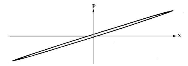
Figure 1: The ellipse represents the typical volume in phase space of the free particle for large times $t$. The length of the ellipse grows to infinity while the width tends to zero. This is equivalent to a classical stochastic process with stochastic positions and fixed corresponding classical momenta. For large times $t$, the ellipse tends to the horizontal position.

Although one has an exact WKB situation for large times, the corresponding wave function possesses large quantum features in the sense, that it is very broad in position. In a slit experiment, for example, one would expect to obtain notable interference fringes. However, for $t\to\infty$, the de Broglie wavelength goes to infinity, and one would have to increase the size of the slit in correspondence to conserve the interference pattern. Remember that while the slit is in position, the squeezing is in momentum. In order to gain more insight into the pattern on the screen behind the slit, we consider now some concrete classical stochastic process. We first specify the probability densities ${\cal P}(p_{0})$ in the initial momenta and ${\cal P}(x_{0})$ in the initial positions of a free classical stochastic particle. Let us consider the following case:

$${\cal P}(p_{0}) = \frac{1}{\sqrt{2\pi}~{}\sigma}~{}e^{-\frac{p_{0}^{2}}{2\sigma^{2}}}$$ (63)

$${\cal P}(x_{0}) = L^{-1}~{}~{}{\rm for}~{}~{}x_{1}-\frac{L}{2}\leq x_{0}\leq x_{1}+\frac{L}{2}\ .$$ (64)

We ask now for the probability ${\cal P}(x(t)\in\Delta x)$ that the free particle will have its position at time $t$ in some interval $\Delta x$ centered around some arbitrary position $x_{1}$. This probability corresponds to all the particles with initial coordinates $(x_{0},p_{0})$ in phase space inside a tilted area (see Figure 2).

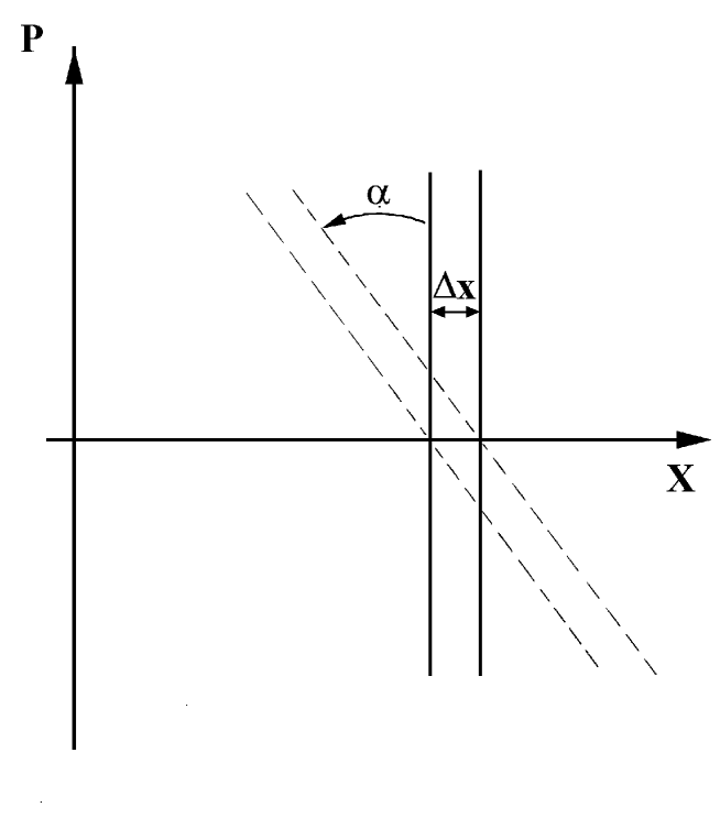
Figure 2: The tilted area corresponds to the points in phase space at time $t=0$ that will eventually have their position $x(t)$ at time $t$ in some interval $\Delta x$. In particular $\alpha=\tan^{-1}\frac{t}{m}$.

As larger times are considered, this area gets increasingly tilted with $\tan\alpha={t}/{m}$. Let us then vary the initial conditions in the positions in such a way that $\frac{L}{2}\frac{m}{t}=N\sigma\equiv\Delta p$, with $N$ sufficiently large. In this way, all the initial momenta $-N\sigma\leq p_{0}\leq N\sigma$ are included in the area and if we include even more momenta, the resulting change in ${\cal P}(x(t)\in\Delta x)$ will be negligible. From the geometry of the problem it is now easy to get the result:

$${\cal P}(x(t)\in\Delta x)=A\frac{m}{t}~{}\Delta x~{},$$ (65)

where

$$A=\frac{1}{\sqrt{2\pi}~{}\sigma}\int\limits^{\Delta p}_{-\Delta p}e^{-\frac{p^{2}}{2\sigma^{2}}}\approx 1~{}.$$ (66)

The range $\Delta x$ can be taken on the screen; actually, the existence of a slit is not important at all for our one-dimensional classical stochastic particle. Indeed, all the allowed classical trajectories (from different tilted areas) will pass through the slit, however at different times. Only the width $\Delta x$ is important and not its location on the screen. The probability per interval $\Delta x$ is constant for given time, while ${\cal P}(x(t)\in\Delta x)\to 0$ for $t\to\infty$. This result is essentially independent from ${\cal P}(x_{0})$ because as $t\to\infty$ more and more possible initial positions are included corresponding to the same momentum $p_{0}$, and hence (65) is recovered independently of the details of ${\cal P}(x_{0})$. This also corresponds to the fact that as $t\to\infty$ the initial positions become negligible compared to ${p_{0}t}/{m}$ so that the details of their probability distribution becomes irrelevant. We have emphasised in [14] that in this limit the classical arrival time of the free particle is much bigger than its quantum indeterminacy (which is inversely proportional to the initial kinetic energy of the particle [21]). The result is finally independent of ${\cal P}(p_{0})$, provided all possible momenta are taken into account.

The quantity ${\cal P}(x(t)\in\Delta x)$ gives us no information about ${\cal P}(p_{0})$; for this we would need a “momentum” slit and ask for the probability that $p(t)\in\Delta p$ at time $t$, which would just give us the probability for $p_{0}\in\Delta p$. This is in sharp contrast with the cosmological perturbations produced during inflation where the various observations of quantities like the matter power spectrum $P(k)$ or the multipoles $C_{\ell}$ of the cosmic microwave background anisotropies give us information about the distribution of the initial amplitudes, the only information we have access to. The relevant initial probability distribution is in the elongated direction (the amplitudes) for the cosmological perturbations, while it is in the squeezed direction (the momenta) for the free particle.

One might wonder whether there are other examples from quantum field theory in external backgrounds where a similar situation occurs as the case of cosmology seems to be very peculiar. Consider, for example, the case of charged scalar particles in an external electromagnetic field (a detailed discussion of the functional Schrödinger picture, similar to the framework employed here, can be found in [22]). The analogous equation to (3) reads there

$$\ddot{y}+[m^{2}+(e{\bf A}+{\bf p})^{2}]y=0\ ,$$ (67)

where ${\bf A}$ denotes the external vector potential, and $m$ is the mass of the charged (scalar) particle. One can have parametric resonance in this case too [23] when $\bf A$ is oscillating. Mathematically, the solution is then the product of an oscillating (periodic) part with a growing or decaying exponential function. When the decaying solution is neglected, a transition to classical behaviour is also obtained.

5 The role of environmental decoherence

The standard way to understand the emergence of classical behaviour in quantum theory is, in contrast to the above example, the interaction of a quantum system with its natural environment [13]. The important point in this context is that most quantum objects cannot be considered as being isolated, but are strongly entangled with the states of the environment. The coupling to the environment may be very small to achieve classical behaviour as the example of the dust grain interacting only with the microwave background [13, 24] demonstrates. Thus, decoherence is an ubiquitous phenomenon.

The actual amount of decoherence depends on the given states and the interaction. Because of the universal interaction of gravity with all other fields, the gravitational field becomes – apart from small fluctuations, the gravitational waves – the most classical quantity. This was in particular shown for the scale factor of a Friedmann Universe whose classicality is a prerequisite for the classicality of other fields [25]. One may call this the hierarchy of classicality, with the (global) gravitational field at the top and small molecules and atoms at the bottom. This quasiclassical nature of the scale factor is a necessary condition for the above cosmological scenario, where the a priori existence of a background spacetime is assumed.

What are the main differences between environment-induced decoherence and the above discussed classicality of the field modes? The squeezed state found above, though it lends itself to a description in classical stochastic terms, is nevertheless a quantum state par excellence (it has, for example, a non-positive Glauder-Sudarshan distribution function). In principle, for large but finite squeezing $|r|$, the coherences are still present in the system itself and could be observed with an appropriate experimental setting, though in the case of inflation $|r|$ is large enough so that these coherences are unobservable in practice. Hence, certainly for the given observational resolution (which eventually are those of the satellite missions mentioned in the introduction) but even well beyond it, the observations cannot be distinguished from those generated by a classical stochastic process as discussed in section 3. On the other hand, for a decohered system one is unable from any practical point of view to observe any coherences in the system itself, although a theoretical, extremely tiny, coherence width always remains. The reason for this is that the coherences are present in the correlations with the environment, and the huge number of degrees of freedom in the environment cannot be controlled.

How can the effect of the environment be quantitatively estimated? A convenient measure for the emergence of quantum entanglement is the rate of de-separation, first introduced in [26] (see also [13]). This is defined as follows. Consider the total system consisting of the relevant part (our “system”) and irrelevant environmental degrees of freedom. The total state $|\Psi\rangle$ can be uniquely expanded as a single sum into (time-dependent) orthonormal basis states of relevant system and environment – the Schmidt expansion:

$$|\Psi(t)\rangle=\sum_{n}\sqrt{p_{n}(t)}|\varphi_{n}^{S}(t)\rangle|\phi_{n}^{S}(t)\rangle\ ,$$ (68)

where $\{\varphi_{n}^{S}\}$ and $\{\phi_{n}^{S}\}$ are the Schmidt basis states of relevant system and environment, respectively. If at some artificial initial time $t=0$ the total state factorises,

$$|\Psi(0)\rangle=|\varphi_{0}\rangle|\phi_{0}\rangle\ ,$$ (69)

the interaction (defined through the Hamiltonian $H$) will in general lead to entanglement: Up to order $t^{2}$ one obtains

$$|\Psi(t)\rangle \approx (1-t^{2}{\cal A})^{1/2}|\varphi_{0}^{S}(t)\rangle|\phi_{0}^{S}(t)\rangle$$ (70)

$$\ +(t^{2}{\cal A})^{1/2}|\varphi_{1}^{S}(t)\rangle|\phi_{1}^{S}(t)\rangle\ ,$$

where

$${\cal A}=\sum_{j\neq 0,m\neq 0}\left|\langle\varphi_{j}\phi_{m}|H|\varphi_{0}\phi_{0}\rangle\right|^{2}$$ (71)

is the rate of de-separation ($\{\varphi_{j}\}$ and $\{\phi_{m}\}$ denote here a fixed orthonormal basis for system and environment, respectively). It is obvious that for ${\cal A}\neq 0$ the total state no longer factorises. The associated decoherence timescale is thus $t_{D}=1/\sqrt{{\cal A}}$. The rate of de-separation can also be related to a different measure of decoherence – the increase of local entropy [13].

If the total Hamiltonain $H$ is of the form

$$H=H_{\varphi}+H_{\phi}+W_{\varphi}\otimes W_{\phi}\ ,$$ (72)

${\cal A}$ is independent of the “free” parts $H_{\varphi}$ and $H_{\phi}$ and can be written in the form

$${\cal A}={\cal A}_{\varphi}{\cal A}_{\phi}\ ,$$ (73)

where

$${\cal A}_{\varphi} = \langle\varphi_{0}|W_{\varphi}^{2}|\varphi_{0}\rangle-\langle\varphi_{0}|W_{\varphi}|\varphi_{0}\rangle^{2}\equiv(\Delta W_{\varphi})^{2}\ ,$$ (74)

$${\cal A}_{\phi} = \langle\phi_{0}|W_{\phi}^{2}|\phi_{0}\rangle-\langle\phi_{0}|W_{\phi}|\phi_{0}\rangle^{2}\equiv(\Delta W_{\phi})^{2}\ .$$ (75)

This is just the mean square deviation of the interaction Hamiltonian $H_{int}\equiv W_{\varphi}\otimes W_{\phi}$ with respect to the initial state. It is this form that we shall use below for our concrete calculations.

What are the relevant interaction Hamiltonians for fields in the early Universe? The details are certainly complicated and depend on the (as yet unkown) precise form of grand unification theories. What is clear from present particle physics models, however, is the fact that the interaction is local in field space (as opposed to field momentum space). Therefore, field amplitudes are “measured” by the environment and one expects large decoherence for states that are broad in field amplitude space (as happens for the squeezed states considered here). This is well known from quantum optics [13] and will be shown to happen also here.

To find a lower bound on the amount of decoherence, it is sufficient to consider a simplified interaction term. We take

$$H_{int}=gk^{2}(y_{\bf k}z^{\dagger}_{\bf k}+y_{\bf k}^{\dagger}z_{\bf k})=2gk^{2}(y_{1}z_{1}+y_{2}z_{2})\ ,$$ (76)

where $g$ is a dimensionless coupling constant, and $z_{\bf k}\equiv z_{1}+\mbox{i}z_{2}$ is the environmental field which is assumed to possess the same “free” part as $y_{\bf k}$. This is similar to the interaction term used in the toy model of [27].

We assume that at some instant the total state is, as in (69), a product state of the $y$-part and the $z$-part,

$$\Psi\equiv\psi_{y_{1}}\psi_{y_{2}}\psi_{z_{1}}\psi_{z_{2}}\ .$$ (77)

For the $y$-part we take our squeezed state produced by inflation, while for the $z$-part we take for simplicity the vacuum state, i.e., with $\Omega$ in the Gaussian given by $\Omega=\Omega_{R}=k$ (the essence of the result remains unchanged by taking more complicated states). The rate of de-separation then becomes

$${\cal A}=(\Delta W_{y_{1}})^{2}(\Delta W_{z_{1}})^{2}+(\Delta W_{y_{2}})^{2}(\Delta W_{z_{2}})^{2}\ ,$$ (78)

where $W_{y_{1}}=\sqrt{2g}ky_{1}$ etc., and the variances are evaluated with respect to the various wave functions in (77). Since

$$\langle\psi_{y_{1}}|y_{1}^{2}|\psi_{y_{1}}\rangle=\frac{|f_{k}|^{2}}{2},\;\langle\psi_{z_{1}}|y_{1}^{2}|\psi_{z_{1}}\rangle=\frac{1}{4k}\ ,\ldots\ ,$$

the rate of de-separation (78) is given by

$${\cal A}=g^{2}k^{3}|f_{k}|^{2}=\frac{g^{2}k^{2}}{2}(\cosh 2r_{k}+\cos 2\varphi_{k}\sinh 2r_{k})\ .$$ (79)

The measure for quantum entanglement is thus essentially given by the power spectrum of the fluctuations! In the limit of large squeezing in $p$-direction ($\varphi_{k}\to 0$) this becomes

$${\cal A}\to\frac{g^{2}k^{2}}{2}\mbox{e}^{2r_{k}}\ .$$ (80)

The corresponding decoherence time is then given by

$$t_{D}\sim\frac{a}{gk\mbox{e}^{r}}\sim\frac{\lambda_{phys}}{g\mbox{e}^{r}}\ ,$$ (81)

where $\lambda_{phys}$ denotes the physical wavelength of the fluctuations. For example, for $\lambda_{phys}\sim 10^{28}\mbox{cm}$ (present horizon scale) and $\mbox{e}^{r}\sim 10^{50}$ (squeezing factor of this mode) one has

$$t_{D}\sim 10^{-31}g^{-1}\mbox{sec}\ ,$$

so that decoherence would be negligible only if one fine-tuned the coupling to values $g\ll 10^{-31}$ – a totally unrealistic fine-tuning!

It is straightforward to extend this analysis to more complicated couplings. Taking, for example, a quadratic coupling,

$$H_{int}=2gk^{3}(y_{1}^{2}z_{1}^{2}+y_{2}^{2}z_{2}^{2})\ ,$$

one finds in the limit of large squeezing for the rate of de-separation

$${\cal A}\to\frac{9}{32}g^{2}k^{2}\mbox{e}^{4r}$$ (82)

which is much bigger than the expression for linear coupling. The decoherence time for the scales which now appear inside the horizon is then

$$t_{D}\sim 10^{-81}g^{-1}\mbox{sec}\ ,$$ (83)

and one would have to fine-tune $g$ even more to have negligible decoherence. We note that $t_{D}$ is proportional to the wavelength of the modes because localisation becomes worse for larger wavelengths [13, 24]. This is, however, largely overcompensated by the high squeezing of these modes due to inflation (the factor $\mbox{e}^{r}$ in the denominator of $t_{D}$).

Due to the nature of the interaction, which is local in field space, the pointer basis defining classical properties is the field amplitude basis and not, for example, the particle number basis. This basis is stable during the dynamical evolution because of the quantum nondemolition condition (16). An analogous example in quantum electrodynamics has been discussed in [29, 30].

To go beyond estimates, one has to take realistic models and calculate the corresponding decoherence times quantitatively, for example by the use of the influence functional method (an introduction to this method can be found in Chap. 5 of [13]). Early investigations of decoherence for primordial fluctuations are [27] and [31]; more recent and more refined calculations can be found in [32, 33] and the references therein. It is, however, of fundamental importance that in order to leave the main predictions of inflation unaltered, interaction with the environment should not destroy the fixed phase of the perturbations, though it can, and certainly will, affect the coherence between growing and decaying mode. In particular, it is crucial that environment-induced decoherence does not produce a density matrix which is diagonal in the basis of number eigenstates [12], as assumed in some of the above quoted references, because in this case the phase becomes random and some basic predictions concerning the CMB anisotropies are dramatically changed (see conclusion).

It is also interesting to calculate the rate of de-separation, if our system is initially in the number eigenstate (26), while for the environmental ($z$-) part the vacuum state is retained. A straightforward calculation using the expressions presented in [11] yields

$${\cal A}_{N}=(2N+1){\cal A}\ ,$$ (84)

with ${\cal A}$ given by (78). Therefore, the rate of de-separation is even stronger than in the vacuum case, as expected.

For Schrödinger cat states (such as the states used recently in quantum optical experiments of decoherence [34]) one would expect an even higher rate of de-separation and even smaller decoherence timescale (cf. Sect. 3.3.3 in [13]).

A good analogy to our case of primordial fluctuations is Fermi’s golden rule and the exponential decay in quantum mechanics [13]. For isolated systems, this is known to hold only approximately, although deviations are hard to measure and have been observed only recently (this would in our example correspond to observe effects of the decaying mode). If, however, the environment is taken into account in this case, exponential decay is enforced by this interaction and no deviations from it can be seen. At the same time, all probabilities remain unchanged. (This would correspond to the impossibility to observe any coherence effects for the primordial fluctuations, while at the same time all probabilities remain unchanged).

We want to finally emphasise again that decoherence can be of importance (due to the emergence of quantum entanglement) long before any dynamical back reaction occurs. This is the reason why all the predictions concerning the primordial fluctuations are unchanged, while at the same time nonclassical interference terms remain essentially suppressed in the system itself. Quantum mechanical examples tell that “decohered” wave packets show no interference even if they occupy the same region of space (see in particular Fig. 3.7 in [13]). Although nonclassical behaviour of squeezed states [35] is difficult to observe for an isolated system (and $|r|$ much smaller than for inflation, otherwise it is hopeless), it is in practice impossible to observe for the decohered system.

6 Conclusions

We have investigated in detail the quantum-to-classical transition of the fluctuations of quantum origin produced during inflation. When no interaction with the environment is taken into account, such a transition takes place up to a precision well beyond observational capabilities. This is directly related to the fact that it is possible to describe the fluctuations nowadays solely with the help of the “growing” quasi-isotropic mode. This transition means that the quantum coherence can be expressed in classical terms, namely the system can be described as a stochastic classical system. That this is very far away from a classical (deterministic) system is very clear in the example of a free particle: at very large times, one cannot ascribe anymore to it a definite trajectory in phase space, but rather one has a classical probability density with stochastic amplitudes (positions) $x$ and fixed momenta $p_{cl}(x)$. The initial quantum state then completely defines the statistics of the fluctuations through the probability distribution $|\Psi|^{2}$. Most inflationary models lead to a Gaussian statistics of the fluctuations, a result in good agreement with observations. Clearly this is very far away from a classical free particle! This aspect is somehow hidden in the case of cosmological fluctuations because in the latter case one is willing to accept the stochasticity of the fluctuations, and it would look absurd to even try a deterministic description of these fluctuations, even if one believes the fluctuations are classical from the very beginning. This explains why the description in terms of a classical stochastic process does not look surprising. It is only when one thinks of the quantum origin of the fluctuations that the peculiar quantum nature appears. We stress also that the quantum-to-classical transition is a result of the expansion of the universe and that it depends on the stretching of the fluctuations while they are outside the Hubble radius. Note that this would not apply to scalar fields with too large mass [36], in complete accordance with the fact that these fields cannot be described by just a growing mode.

We again emphasise that the environment has to be taken into account, since the highly squeezed states are extremely sensitive to the presence of an environment, as has been discussed in Sect. 5. When it is taken into account, even coherences which are unobservable in practice but still present in the system, essentially disappear from the system itself, since they are “hidden” in the correlations with the huge number of degrees of freedom of the environment. However, in the peculiar case of inflation these coherences, not expressible in classical stochastic terms, are anyway tremendously tiny. It is not even clear that environment-induced decoherence would be effective enough to reduce them any further. However, interaction with the environment has an irreversible character and is certainly crucial regarding the problem of the entropy of the fluctuations. It is crucial that this interaction does not spoil the standard predictions of inflationary physics which will be possibly tested in the near future by the satellite missions MAP and, with even higher accuracy, by PLANCK Surveyor. For example, the fact that the fluctuations have stochastic amplitudes but fixed phases results in the appearance of (Sakharov or Doppler or acoustic) peaks on small angular scales in the angular power spectrum of the cosmic microwave background anisotropies.

We note that our discussions exhibit a surprising connection between cosmology – the origin of structure – and fundamentals of quantum theory [14]. The quantum-to-classical transition by decoherence is a very general process as studied recently in quantum optical experiments [34].

We emphasised in Sect. 2 that the high squeezing of the quantum state for the primordial fluctuations is “generic”. One can, of course, start with any “quantum state” at the end of inflation (not necessarily highly squeezed) and evolve it back to the beginning of inflation by the Schrödinger equation, where it yields an acceptable initial state. However, this state should initially (before inflation) be tremendously narrow in $y$ and may be rejected as being unnatural (this is our quantum no hair conjecture). Assuming that such an initial state is self consistent with inflation, which is certainly not the case for most models, then the longer the inflationary phase, the better our conjecture is expected to work; however, the minimum duration required for inflation to be of cosmological interest is certainly effective enough in this respect. The high squeezing of the fluctuations and the ensuing quantum-to-classical transition is a generic feature of the inflationary phase itself.

References

- [1] A. Linde, Rep. Prog. Phys. 47, 925 (1984); Particle physics and inflationary cosmology (Harwood, New York, 1990); E. Kolb, M. Turner, The Early Universe (Addison-Wesley, Redwood City, 1990).
- [2] S.W. Hawking, Phys. Lett. B 115, 295 (1982); A.A. Starobinsky, Phys. Lett. B 117, 175 (1982); A.H. Guth and S-Y. Pi, Phys. Rev. Lett. 49, 1110 (1982).
- [3] http://astro.estec.esa.nl/SA-general/Projects/Planck/
- [4] http://map.gsfc.nasa.gov/
- [5] G. Börner and S. Gottlöber (eds.), The Evolution of the Universe (John Wiley, Chichester, 1997).
- [6] A.A. Starobinsky, JETP Lett. 30, 682 (1979).
- [7] C. Kiefer and T.P. Singh, Phys. Rev. D 44, 1067 (1991); A.O. Barvinsky and C. Kiefer, Nucl. Phys. B 526, 509 (1998).
- [8] J.L. Rosales, Phys. Rev. D 55, 4791 (1997).
- [9] A. Albrecht, Report hep-th/9402062.
- [10] D. Polarski and A.A. Starobinsky, Class. Quantum Grav. 13, 377 (1996).
- [11] J. Lesgourgues, D. Polarski, and A.A. Starobinsky, Nucl. Phys. B 497, 479 (1997).
- [12] J. Lesgourges, D. Polarski, and A.A. Starobinsky, Class. Quantum Grav. 14, 881 (1997).
- [13] D. Giulini, E. Joos, C. Kiefer, J. Kupsch, I.-O. Stamatescu, and H.D. Zeh, Decoherence and the Appearance of a Classical World in Quantum Theory (Springer, Berlin, 1996).
- [14] C. Kiefer, D. Polarski, and A.A. Starobinsky, Int. Journ. Mod. Phys. D 7, 455 (1998).
- [15] L.P. Grishchuk and Y.V. Sidorov, Phys. Rev. D 42, 3413 (1990); see also L.P. Grishchuk, Class. Quantum Grav. 10, 2449 (1993).
- [16] B. Schumaker, Phys. Rep. 135, 317 (1986).
- [17] D.F. Walls and G.J. Milburn, Quantum Optics (Springer, Berlin, 1994).
- [18] R. Jackiw, Diverse Topics in Theoretical and Mathematical Physics, Sect. IV.4 (World Scientific, Singapore, 1995).
- [19] A. Albrecht, P. Ferreira, M. Joyce, and T. Prokopec, Phys. Rev. D 50, 4807 (1994).
- [20] D. Polarski and A.A. Starobinsky, Phys. Lett. B 356, 196 (1995).
- [21] Y. Aharonov, J. Oppenheim, S. Popescu, B. Reznik, and W.G. Unruh, Report quant-ph/9709031, to appear in Phys. Rev. A.
- [22] C. Kiefer, Phys. Rev. D 45, 2044 (1992).
- [23] L. Kofman, A. Linde, and A.A. Starobinsky, Phys. Rev. Lett. 73, 3195 (1994); Phys. Rev. D 56, 3258 (1997); P. Greene, L. Kofman, A. Linde, and A.A. Starobinsky, Phys. Rev. D 56, 6175 (1997).
- [24] E. Joos and H.D. Zeh, Z. Phys. B 59, 223 (1985).
- [25] C. Kiefer, Class. Quantum Grav. 4, 1369 (1987).
- [26] O. Kübler and H.D. Zeh, Ann. Phys. (N.Y.) 76, 405 (1973).
- [27] R. Brandenberger, R. Laflamme, and M. Mijić, Mod. Phys. Lett. A 5, 2311 (1990).
- [28] M.N. Nieto, Phys. Lett. A 229, 135 (1997).
- [29] C. Kiefer, Phys. Rev. D 46, 1658 (1992).
- [30] J.R. Anglin and W.H. Zurek, Phys. Rev. D 53, 7327 (1996).
- [31] M. Sakagami, Progr. Theor. Phys. 79, 442 (1988); H.A. Feldman and A. Yu. Kamenshchik, Class. Quantum Grav. 8, L65 (1991); H.A. Feldman, A. Yu. Kamenshchik, and A.I. Zelnikov, Class. Quantum Grav. 9, L1 (1992).
- [32] E. Calzetta and B.L. Hu, Phys. Rev. D 52, 6770 (1995); E.A. Calzetta and S. Gonorazky, ibid. 55, 1812 (1997); A. Matacz, ibid. 55, 1860 (1997).
- [33] D. Boyanovsky and H.J. de Vega, Phys. Rev. D 57, 2166 (1998).
- [34] M. Brune, E. Hagley, J. Dreyer, X. Maître, A. Maali, C. Wunderlich, J.M. Raimond, and S. Haroche, Phys. Rev. Lett. 77, 4887 (1996).
- [35] J.P. Dowling, W. Schleich, and J.A. Wheeler, Ann. Physik (7th series) 48, 423 (1991).
- [36] M. Mijić, Phys. Rev. D 57, 2138 (1998).