Black Holes with Scalar Hair in $(2+1)$ dimensions

Abstract

Nonrotating and rotating black hole soltuions in $(2+1)$ dimensions are studied in a model including a real scalar field with a simple potential coupled to gravity.

I Introduction

In recent years, gravity in three dimensions has attracted much attention. Since Bañados, Teitelboim and Zanelli (BTZ) found circularly-symmetric black hole solutions for three dimensional gravity with a negative cosmological constant [1], properties of their black holes [2] and many other types of three dimensional black holes have been investigated.

On the other hand, static black hole solutions including matter fields in $(3+1)$ dimensions have been examined by many authors. One of their examples is the Yang-Mills black hole in four dimensional spacetime [3]. Its properties have been studied and some descendants have been considered recently [4].

Static black holes with a nontrivial scalar field as a source of gravity is, however, problematic in four dimensions. Beckenstein established a no-go theorem for static spherical black holes with such “scalar hair” in $(3+1)$ dimensions [5].

Again we turn to the three dimensional case. Since BTZ used a negative cosmological constant and found the asymptotically no-flat black hole solution, we do not have to restrict ourselves to the positive definite scalar potentials. Thus the no-go theorem of Bekenstein will be evaded in the three dimensional case. Actually, three-dimensional black hole slutions with scalar fields are studied in various contexts [6, 7, 8].

In the present paper, we considered a simple class of scalar potentials in three dimensional gravity and construct circularly-symmetric black hole solutions in the model. In three dimensions, rotating solutions are most easily treated. Therefore we also consider circularly symmetric rotating black holes with the scalar field.

The action of our model is

$$S=\int d^{3}x\sqrt{-g}\left[\frac{1}{16\pi G}R-\frac{1}{2}(\nabla\phi)^{2}-V(\phi)\right],$$ (1)

where $R$ is the scalar curvature and $\phi$ stands for a real scalar field. $G$ is the Newton’s gravitational constant.

We assume that the potential $V(\phi)$ takes the form:

$$V(\phi)=\left\{\begin{array}[]{ccc}-\frac{1}{2}\mu^{2}\phi^{2}&{}{}{}\hfil&\phi<\phi_{B},\\ \infty&{}{}{}\hfil&\phi>\phi_{B}.\end{array}\right.$$ (2)

A schematic view of the potential is given in FIG. 1.

In the far region from the black hole, $\phi$ falls into the bottom of the potential, $\phi=\phi_{B}$. Therefore in the asymptotic region, the spacetime is the BTZ black hole spacetime with an effective negative cosmological constant $-\lambda=-(8\pi G)\mu^{2}\phi_{B}^{2}/2$.

In Sec. II in the present paper, we derive nonrotating circularly-symmetric solutions in the model. Rotating black holes are analyzed in this model in Sec. III. The last section IV is devoted to a brief conclusion.

II Nonrotating black holes with scalar hair

For the static, nonrotating, circularly-symmetric solutions, the metric can be taken as

$$ds^{2}=-e^{-2\delta(r)}\Delta(r)dt^{2}+\frac{1}{\Delta(r)}dr^{2}+r^{2}d\theta^{2}.$$ (3)

We also assume $\phi$ is a function only of the radial coodinate $r$.

One can obtain the field equations by varying the action (1). When the assumption above is taken into consideration, the field equations can be written as

$$\frac{1}{2r}\frac{d\Delta}{dr} = 8\pi G\left[-\frac{1}{2}\Delta\left(\frac{d\phi}{dr}\right)^{2}-V(\phi)\right],$$ (4)

$$\frac{1}{r}\frac{d\delta}{dr} = 8\pi G\left[-\left(\frac{d\phi}{dr}\right)^{2}\right],$$ (5)

$$\frac{1}{re^{-\delta}}\frac{d}{dr}\left[re^{-\delta}\Delta\frac{d\phi}{dr}\right] = \frac{\partial V}{\partial\phi}.$$ (6)

Now we will introduce dimensionless variables. We choose

$$\tilde{\phi}=\sqrt{8\pi G}\phi,~{}~{}~{}\tilde{r}=r/r_{H},~{}~{}~{}\tilde{\Delta}=\frac{\Delta}{\mu^{2}r_{H}^{2}},$$ (7)

where $r_{H}$ is the radius of the horizon, i.e., $\Delta(r_{H})=0$. Using these variables, the field equations (4-6) can be rewritten, when $\phi<\phi_{B}$, as

$$\frac{1}{\tilde{r}}\tilde{\Delta}^{\prime} = -\tilde{\Delta}\left(\tilde{\phi}^{\prime}\right)^{2}+\tilde{\phi}^{2},$$ (8)

$$\frac{1}{\tilde{r}}\delta^{\prime} = -\left(\tilde{\phi}^{\prime}\right)^{2},$$ (9)

$$\frac{1}{\tilde{r}e^{-\delta}}\left[\tilde{r}e^{-\delta}\tilde{\Delta}\tilde{\phi}^{\prime}\right]^{\prime} + \tilde{\phi}=0,$$ (10)

where a prime (^′) denotes the derivative $d/d\tilde{r}$.

In the region $r_{H}<r<r_{B}$, the value of $\phi$ varies with the radial coordinate, while $\phi$ takes the constant value $\phi=\phi_{B}$ outside the boundary $r=r_{B}$. Then the field equation for $\tilde{r}>\tilde{r}_{B}=r_{B}/r_{H}$ is

$$\frac{1}{\tilde{r}}\tilde{\Delta}^{\prime} = \tilde{\phi}_{B}^{2},$$ (11)

$$\delta^{\prime} = 0,$$ (12)

$$\tilde{\phi} = \tilde{\phi}_{B},$$ (13)

where $\tilde{\phi}_{B}=\sqrt{8\pi G}\phi_{B}$. At the boundary $\tilde{r}=\tilde{r}_{B}$, the interior and exterior solutons must be smoothly continued: thus $\tilde{\phi}^{\prime}=0$ at $\tilde{r}=\tilde{r}_{B}$.

To solve the differential equations (8-10), one must find a suitable set of boudary conditions for a black hole solution. A natural choice of the starting point is $\tilde{r}=1$. This point corresponds to the horizon of the black hole, i.e., $\tilde{\Delta}(1)=0$. The value of $\delta$ moves obviously within a finite range. In the exterior region $\tilde{r}>\tilde{r}_{B}$, $\delta$ takes a constant value. In the region, the spacetime is the vacuum solution of pure gravity with an effective cosmological constant $-(8\pi G)\mu^{2}\phi_{B}^{2}/2$. A constant shift of $\delta$ can be absorbed by redefinition of $t$. Thus we choose $\delta(1)=0$.

We can arbitrarily choose $\tilde{\phi}_{H}=\tilde{\phi}(1)<0$. Then we find that the condition for $\tilde{\phi}^{\prime}(1)$ is

$$\tilde{\phi}^{\prime}(1)=-\frac{\tilde{\phi}_{H}}{\tilde{\Delta}^{\prime}(1)}.$$ (14)

As a consequence of Eq. (8), this equation is reduced to

$$\tilde{\phi}^{\prime}(1)=-\frac{1}{\tilde{\phi}_{H}}.$$ (15)

Under these conditions, we can solve the equations (8-10) numerically. If we choose a value of $\tilde{\phi}_{H}$, $\tilde{r}_{B}$ is determined by a numerical calculation: it is the value of the radial coordinate which fulfills $\tilde{\phi}^{\prime}(\tilde{r}_{B})=0$. $\tilde{\phi}_{B}$ is given by the value $\tilde{\phi}(\tilde{r}_{B})$.

The numerical solutions of $\tilde{\phi}$, $\tilde{\Delta}$, and $\delta$ for a specific value $\tilde{\phi}_{H}=-1$ are shown in FIG. 2.

The properties of a black hole solution are extracted from the value of the variables at $\tilde{r}=\tilde{r}_{B}$. In the exterior region, the variables are ones of the BTZ black hole solution except for the scaling of the time coordinate due to $\delta$. The smooth connection at the boundary determines the mass of the black hole $M$. We obtain:

$$\frac{8GM}{\mu^{2}r_{H}^{2}}=\frac{1}{2}\tilde{\phi}_{B}^{2}\tilde{r}_{B}^{2}-\tilde{\Delta}_{B},$$ (16)

where $\tilde{\Delta}_{B}=\tilde{\Delta}(\tilde{r}_{B})$. The effective cosmological constant is given by

$$\frac{\lambda}{\mu^{2}}=\frac{1}{2}\tilde{\phi}_{B}^{2}.$$ (17)

The black hole solution has the three characteristic length scale; $r_{H}$, $r_{B}$, and the horizon radius of the BTZ black hole which has the same mass and cosmological constant, i.e.,

$$r_{H0}=\sqrt{\frac{8GM}{\lambda}}.$$ (18)

The ratios of $r_{H}^{2}/r_{H0}^{2}$ is plotted as a function of $\lambda/\mu^{2}$ in FIG. 3. In FIG. 4, $r_{H}^{2}/r_{B}^{2}$ and $r_{H0}^{2}/r_{B}^{2}$ are shown as functions of $\lambda/\mu^{2}$. For a large value of $\lambda/\mu^{2}$, the present type of the black hole cannnot exist. The critical value is approximately given by $\lambda/\mu^{2}\approx 0.042$.

On the other hand, in the limit of small $\lambda/\mu^{2}$, all the ratios converge to unity. Then the effect of “scalar hair” tends to be small and the black hole approaches a usual BTZ black hole in the limit $\lambda/\mu^{2}\rightarrow 0$.

The Hawking temperature of the black hole is proportional to the strength of the surface gravity at the horizon. Practically speaking, the Hawking temperature $T$ is derived from the condition that the Euclideanized metric has no conical singularity at the horizon when the Euclidean time has the period $1/T$. In the present case, $T$ is given as

$$\frac{T}{\mu^{2}r_{H}}=\frac{1}{4\pi}e^{\delta_{B}}\tilde{\phi}_{H}^{2}.$$ (19)

Here the dependence on $\delta_{B}=\delta(\tilde{r}_{B})$ comes from the redefinition of $t$, which converts the exterior solution into the BTZ solution explicitly.

In FIG. 5, we show the ratio $T^{2}/T_{0}^{2}$, where $T_{0}$ is the Hawking temperature of the BTZ black hole of the same mass and cosmological constant [1]:

$$T_{0}=\frac{\sqrt{8GM\lambda}}{2\pi}.$$ (20)

The ratio $T^{2}/T_{0}^{2}$ is always larger than unity for a finite value of $\lambda/\mu^{2}$ less than the critical value. The ratio grows up if the value of $\lambda/\mu^{2}$ approaches to the critical value, $\lambda/\mu^{2}\approx 0.042$. In the limit of small $\lambda/\mu^{2}$, the ratio becomes unity.

III Rotating black holes with scalar hair

For the rotating, circularly-symmetric solutions, the metric can be taken as

$$ds^{2}=-e^{-2\delta(r)}\Delta(r)dt^{2}+\frac{1}{\Delta(r)}dr^{2}+r^{2}\left(d\theta-\Omega(r)dt\right)^{2},$$ (21)

We also assume $\phi$ is the function of the radial coodinate. Note that under the circularly-symmetric ansatz, a real scalar cannot depend on the angular variable.

One can obtain the field equations by taking variations of the action (1) under the circularly-symmetric ansatz. Since the $(0,2)$ component of Einstein equation does not include $\phi$ dependence in our case, the equation can be integrated and leads to

$$e^{2\delta}\left(\frac{d\Omega}{dr}\right)^{2}=\frac{(8GJ)^{2}}{r^{6}},$$ (22)

where $J$ is a constant. $J$ turns out to be the value of the angular momentum of the black hole[1].

Other field equations can be rewritten by using the dimensionless variables as in the previous section. In this time we take

$$\tilde{\phi}=\sqrt{8\pi G}\phi,~{}~{}~{}\tilde{r}=r/r_{H},~{}~{}~{}\tilde{\Delta}=\frac{\Delta}{\mu^{2}r_{H}^{2}},~{}~{}~{}and~{}~{}~{}\tilde{J}=\frac{8GJ}{\mu r_{H}^{2}}.$$ (23)

Using these variables, the field equations for $\phi<\phi_{B}$ can be read as

$$\frac{1}{\tilde{r}}\tilde{\Delta}^{\prime} = -\tilde{\Delta}\left(\tilde{\phi}^{\prime}\right)^{2}+\tilde{\phi}^{2}-\frac{\tilde{J}^{2}}{2\tilde{r}^{4}},$$ (24)

$$\frac{1}{\tilde{r}}\delta^{\prime} = -\left(\tilde{\phi}^{\prime}\right)^{2},$$ (25)

$$\frac{1}{\tilde{r}e^{-\delta}}\left[\tilde{r}e^{-\delta}\tilde{\Delta}\tilde{\phi}^{\prime}\right]^{\prime} + \tilde{\phi}=0.$$ (26)

As in the nonrotating case, $\phi$ takes the constant value $\phi=\phi_{B}$ in the exterior region of the boundary $r=r_{B}$. Then the field equation for $\tilde{r}>\tilde{r}_{B}=r_{B}/r_{H}$ is

$$\frac{1}{\tilde{r}}\tilde{\Delta}^{\prime} = \tilde{\phi}_{B}^{2}-\frac{\tilde{J}^{2}}{2\tilde{r}^{4}},$$ (27)

$$\delta^{\prime} = 0,$$ (28)

$$\tilde{\phi} = \tilde{\phi}_{B},$$ (29)

where $\tilde{\phi}_{B}=\sqrt{8\pi G}\phi_{B}$. The smooth connection of the interior and exterior solutons must be required.

A suitable set of boudary conditions for solving the differential equations (24-26) can be found as in the previous case. At $\tilde{r}=1$, we set $\tilde{\Delta}(1)=0$, $\delta(1)=0$, and

$$\tilde{\phi}^{\prime}(1) = -\frac{\tilde{\phi}_{H}}{\tilde{\Delta}^{\prime}(1)}$$ (30)

$$= -\frac{\tilde{\phi}_{H}}{\tilde{\phi}_{H}^{2}-\frac{\tilde{J}^{2}}{2}}.$$ (31)

The properties of a rotating black hole solution can be extracted from the numerical value of the variables at $\tilde{r}=\tilde{r}_{B}$ as previously. In the exterior region, the solution is the rotating BTZ black hole solution [1]. By examining the connection condition, we find:

$$\frac{8GM}{\mu^{2}r_{H}^{2}}=\frac{1}{2}\tilde{\phi}_{B}^{2}\tilde{r}_{B}^{2}+\frac{\tilde{J}^{2}}{4\tilde{r}_{B}^{2}}-\tilde{\Delta}_{B},$$ (32)

and the effective cosmological constant is again given by

$$\frac{\lambda}{\mu^{2}}=\frac{1}{2}\tilde{\phi}_{B}^{2}.$$ (33)

The horizon radius of the rotating BTZ black hole with the same mass, angular momentum, and cosmological constant is given by

$$r_{H0}=\sqrt{\frac{1}{2}\left(\frac{\bar{M}}{\lambda}+\sqrt{\frac{\bar{M}^{2}}{\lambda^{2}}-\frac{\bar{J}^{2}}{\lambda}}\right)},$$ (34)

where

$$\bar{M}=8GM~{}~{}~{}and~{}~{}~{}\bar{J}=8GJ.$$ (35)

The ratios $r_{H}^{2}/r_{H0}^{2}$ for rotating black holes are plotted in FIG. 6. In FIG. 7, the values of $r_{H}^{2}/r_{B}^{2}$ and $r_{H0}^{2}/r_{B}^{2}$ for rotating black holes are plotted.

In these figures, the $x$-axis indicates $\lambda/\mu^{2}$ while $y$-axis $J^{2}\lambda/M^{2}$. In these figures, the sequences of the points correspond to $\frac{8GJ}{\mu r_{H}}=0.1,0.2,0.3,0.4,0.5,0.6,0.7,0.8,0.9,$ and $1$.

It is worth noting that the scattered points, which correspond to different solutions, lie within the range $0<J^{2}\lambda/M^{2}<1$. The same restriction hold for the rotating BTZ black hole solution (with the horizon) [1].

In the rotating case, the Hawking temperature $T$ is given by

$$\frac{T}{\mu^{2}r_{H}}=\frac{1}{4\pi}e^{\delta_{B}}\left(\tilde{\phi}_{H}^{2}-\frac{\tilde{J}^{2}}{2}\right).$$ (36)

In FIG. 8, we show the ratio $T^{2}/T_{0}^{2}$, where $T_{0}$ is the Hawking temperature of the BTZ black hole of the same mass, angular momentum and cosmological constant [1]:

$$T_{0}=\frac{\lambda}{2\pi r_{H0}}\sqrt{\frac{\bar{M}^{2}}{\lambda^{2}}-\frac{\bar{J}^{2}}{\lambda}}.$$ (37)

Again the $x$-axis indicates $\lambda/\mu^{2}$ while $y$-axis $J^{2}\lambda/M^{2}$ in FIG. 8.

What does the result mean? Now FIG. 9 shows the scattered points in FIG. 6 projected onto the $\lambda/\mu^{2}$-$r_{H}^{2}/r_{H0}^{2}$ plane. The points are laid on a curve, which is the same curve in the nonrotating case. Similarly, in FIG. 10 the projected points of FIG. 7 are shown. The ratios $r_{H}^{2}/r_{B}^{2}$ and $r_{H0}^{2}/r_{B}^{2}$ depend on the ratio of the angular momentum and mass of the black hole. In FIG. 11 the projected points of FIG. 8 are shown. The ratio $T^{2}/T_{0}^{2}$ does not depend on the ratio of the angular momentum and mass of the black hole.

In summary, $r_{H}^{2}/r_{H0}^{2}$ and $T^{2}/T_{0}^{2}$ are independent of the value of angular momentum. Therefore the critical value of $\lambda/\mu^{2}$ is the same as the one of the nonrotating case, $\lambda/\mu^{2}\approx 0.042$. On the other hand, $r_{H}^{2}/r_{B}^{2}$ and $r_{H0}^{2}/r_{B}^{2}$ depend on the ratio of the angular momentum and mass of the black hole. For larger angular momenta, the ratios become larger.

IV Conclusion

We have constructed circularly-symmetric black hole solutions with scalar hair in $(2+1)$ dimensions. In our model, ratios of physical quantities have dependence on the scaled cosmological constant $\lambda/\mu^{2}$, because of the simplicity of the scalar potential. This fact tells us that the complexity in the behavior of the physical quantities in the case of the Yang-Mills black holes in $(3+1)$ dimensions [3, 4] is due to the non-linear nature of the self-interaction.

Although our model is very simple, we found the critical behavior with respect to $\lambda/\mu^{2}$. We have to study more closely this behavior and the structure of the spacetime when $\lambda/\mu^{2}$ approaches the critical value $\approx 0.042$.

For rotating black holes, we found some ratios of the physical quantities are independent of the angular momentum. The extreme condition seems the same as the one of the vacuum case, $J^{2}\lambda/M^{2}=1$. Studying the structure of the spacetime in the extreme case is of much interest.

Analyzing the stability of our solution is, unfortunately, somewhat difficult because of the singular point in the potential. The general cases with “smooth” potentials must be investigated and the relation to the model of the unified field theory has to be clarified.

FIG. 1.: A schematic view of the scalar potential.

FIG. 2.: The solutions of $\tilde{\phi}$ (the solid line), $\tilde{\Delta}$ (the broken line), and $\delta$ (the dotted line) for $\tilde{\phi}_{H}=-1$.

FIG. 3.: $r_{H}^{2}/r_{H0}^{2}$ as a function of $\lambda/\mu^{2}$.

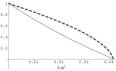
FIG. 4.: $r_{H}^{2}/r_{B}^{2}$ (the solid line) and $r_{H0}^{2}/r_{B}^{2}$ (the gray broken line) as functions of $\lambda/\mu^{2}$.

FIG. 5.: $T^{2}/T_{0}^{2}$ as a function of $\lambda/\mu^{2}$.

FIG. 6.: $r_{H}^{2}/r_{H0}^{2}$ as a function of $\lambda/\mu^{2}$ and $J^{2}\lambda/M^{2}$ for rotating black holes.

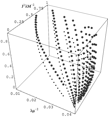
FIG. 7.: $r_{H}^{2}/r_{B}^{2}$ and $r_{H0}^{2}/r_{B}^{2}$ as functions of $\lambda/\mu^{2}$ and $J^{2}\lambda/M^{2}$ for rotating black holes. The small dots represent $r_{H}^{2}/r_{B}^{2}$, while the large gray dots represent $r_{H0}^{2}/r_{B}^{2}$.

FIG. 8.: $T^{2}/T_{0}^{2}$ as a function of $\lambda/\mu^{2}$ and $J^{2}\lambda/M^{2}$ for rotating black holes.

FIG. 9.: $r_{H}^{2}/r_{H0}^{2}$ as a function of $\lambda/\mu^{2}$ for rotating black holes. This is the same as FIG. 6, but projected onto a plane.

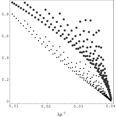
FIG. 10.: $r_{H}^{2}/r_{B}^{2}$ and $r_{H0}^{2}/r_{B}^{2}$ as functions of $\lambda/\mu^{2}$ for rotating black holes. The small dots represent $r_{H}^{2}/r_{B}^{2}$, while the large gray dots represent $r_{H0}^{2}/r_{B}^{2}$. This is the same as FIG. 7, but projected onto a plane.

FIG. 11.: $T^{2}/T_{0}^{2}$ as a function of $\lambda/\mu^{2}$ for rotating black holes. This is the same as FIG. 8, but projected onto a plane.

REFERENCES

[1] M. Bañados, C. Teitelboim and J. Zanelli,
Phys. Rev. Lett. 69, 1849 (1992);
M. Banados, M. Henneaux, C. Teitelboim and J. Zanelli,
Phys. Rev. D48, 1506 (1993).
[2] S. Carlip, Class. Quant. Grav. 12, 2853 (1995)
gr-qc/9506079.
[3] M. S. Volkov and D. V. Gal’tsov, JETP Lett. 50,
346 (1989); Sov. J. Nucl. Phys. 51, 747 (1990);
P. Bizon, Phys. Rev. Lett. 64, 2844 (1990);
H. P. Künzle and A. K. Masoud-ul-Alam,
J. Math. Phys. 31, 928 (1990);
[4] T. Torii and K. Maeda, Phys. Rev. D48,
1643 (1993).
[5] J. D. Bekenstein, Phys. Rev. D51, R6608 (1995).
[6] K.C.K. Chan and R.B. Mann, Phys. Rev. D50,
6385 (1994); D52, 2600(E) (1995); Phys. Lett. B371,
199 (1996).
[7] C Martínez and J. Zanelli, Phys. Rev. D54,
3830 (1996).
[8] K.C.K. Chan, Phys. Rev. D55, 3564 (1997).