The late-time singularity inside non-spherical black holes

Abstract

It was long believed that the singularity inside a realistic, rotating black hole must be spacelike. However, studies of the internal geometry of black holes indicate a more complicated structure is typical. While it seems likely that an observer falling into a black hole with the collapsing star encounters a crushing spacelike singularity, an observer falling in at late times generally reaches a null singularity which is vastly different in character to the standard Belinsky, Khalatnikov and Lifschitz (BKL) spacelike singularity [V. A. Belinsky, I. M. Khalatnikov, and E. M. Lifshitz, Sov. Phys. JETP 32, 169 (1970)]. In the spirit of the classic work of BKL we present an asymptotic analysis of the null singularity inside a realistic black hole. Motivated by current understanding of spherical models, we argue that the Einstein equations reduce to a simple form in the neighborhood of the null singularity. The main results arising from this approach are demonstrated using an almost plane symmetric model. The analysis shows that the null singularity results from the blueshift of the late-time gravitational wave tail; the amplitude of these gravitational waves is taken to decay as an inverse power of advanced time as suggested by perturbation theory. The divergence of the Weyl curvature at the null singularity is dominated by the propagating modes of the gravitational field, that is

$$C_{\alpha\beta\gamma\delta}C^{\alpha\beta\gamma\delta}\sim\Psi_{0}\Psi_{4}\sim v^{-(2l+3)}e^{2\kappa v}$$

as $v\rightarrow\infty$ at the Cauchy horizon. Here, $\Psi_{0}$ and $\Psi_{4}$ are the Newman-Penrose Weyl scalars, and $l\geq 2$ is the multipole order of the perturbations crossing the event horizon. The null singularity is weak in the sense that tidal distortion remains bounded along timelike geodesics crossing the Cauchy horizon. These results are in agreement with previous analyses of black hole interiors. We briefly discuss some outstanding problems which must be resolved before the picture of the generic black hole interior is complete.

I Introduction

Spacetime singularities are an inevitable consequence of the Einstein field equations. They mark the boundary of spacetime, and the limit of our current understanding of gravitational physics. Unfortunately, the powerful techniques used to demonstrate the existence of singularities say nothing about the character of these physical blemishes [1].

The classic works of Belinsky, Khalatnikov and Lifschitz [2] address this deficiency by integrating Einstein’s equations in the neighborhood of a spacelike singularity. They present compelling evidence that the general solution takes an inhomogeneous Kasner form exhibiting chaotic oscillations of the Kasner axes as a crushing singularity is approached [2]. The functional genericity of the BKL solutions is widely interpreted as indicating that all physical singularities must be of this form.

Nonetheless, studies of the internal geometry of black holes suggest a picture involving two distinct regimes. Observers falling into the black hole with the collapsing star generally encounter a spacelike singularity (which is presumably of the BKL type). On the other hand, observers that fall in at late times, when the external geometry has settled down to an almost stationary state, encounter a weak, null singularity of a type similar to the mass-inflation singularity of Poisson and Israel [3].

To understand this behavior we must first discuss the formation of a black hole by the gravitational collapse of a rotating star. At late times, the external gravitational field is believed to settle down to a Kerr-Newman solution. These solutions have a timelike singularity which is preceded by a Cauchy horizon—a null hypersurface marking the boundary of the domain of dependence for Cauchy data prescribed in the black hole exterior. The Cauchy horizon is non-singular, and the spacetime can be analytically extended through it. The global solution then suggests that black holes act as tunnels from our asymptotically flat universe to other identical, but distinct, universes. Indeed there is an infinite lattice of universes extending into the past and future of our own. Furthermore, observers may travel through the ring singularity inside these black holes, passing to achronal regions of spacetime.

In the late 1960’s Penrose pointed out that the Cauchy horizon inside such a black hole is unstable [6]. Time-dependent perturbations originating outside the black hole get infinitely blueshifted as they propagate inwards near to the Cauchy horizon, consequently, the energy density associated with these perturbations diverges as measured by a free-falling observer attempting to cross through the horizon. Perturbative calculations [7] in Reissner-Nordström and Kerr spacetimes have validated Penrose’s original arguments.

In general, gravitational collapse is expected to be asymmetric, so that gravitational and electro-magnetic waves are emitted by a newly formed black hole as it settles down to a stationary, axisymmetric state. Detailed studies of perturbations of black hole geometries show that such gravitational wave emission results in wave tails which decay according to an inverse power law of time in the exterior of the black hole [8, 9]. Some of this radiation inevitably crosses the event horizon getting infinitely blueshifted near to the Cauchy horizon. For this reason one might expect the internal geometry of a black hole formed by collapse is significantly different to that of the exact stationary solutions.

A Spherical models of black hole interiors

The first attempts to understand the back-reaction of the blueshifted, radiative tail on the internal geometry of black holes were restricted to spherical symmetry. Hiscock [10] argued that Isaacson’s [11] effective stress-energy description of high-frequency gravitational waves should be valid near the Cauchy horizon. He considered a charged black hole with a directed influx of lightlike dust with stress-energy tensor $T_{\alpha\beta}=\rho_{\rm in}\ell_{\alpha}\ell_{\beta}$ where $\ell_{\alpha}\ell^{\alpha}=0$, and showed that an observer dependent singularity forms along the Cauchy horizon in this circumstance.

In reality, some of the infalling radiation is back-scattered off the curvature inside the event horizon. Poisson and Israel [3] modeled this effect by another flux of lightlike dust moving to the right; they demonstrated, for the first time, that non-linear effects transform the Cauchy horizon into a scalar curvature singularity. It is worth summarizing the essence of their argument here.

Figure 1 shows the setting for the characteristic initial value problem. Charged ingoing and outgoing Vaidya solutions in regions II and III, respectively, are matched continuously onto region I, which is described by a static Reissner-Nordström solution with mass $m_{0}$ and charge $q$. (The pure ingoing region, II, was studied by Hiscock.) In region IV the line element can be written as

$$ds^{2}=-2e^{\lambda}dudv+r^{2}(d\theta^{2}+\sin^{2}\theta d\phi^{2})\;,$$ (1)

where $r=r(u,v)$ and $\lambda=\lambda(u,v)$. The coordinates are chosen so that $v$ is standard advanced time, i.e. $v=\infty$ at future null infinity, and the retarded time $u=-\infty$ on the black hole event horizon. The stress-energy of cross-flowing null dust is

$$T_{\alpha\beta}=\frac{L_{\rm in}(v)}{4\pi r^{2}}\ell_{\alpha}\ell_{\beta}+\frac{L_{\rm out}(u)}{4\pi r^{2}}n_{\alpha}n_{\beta}\;,$$ (2)

where $\ell_{\alpha}=-\partial_{\alpha}v$ and $n_{\alpha}=-\partial_{\alpha}u$. The luminosity function $L_{\rm in}(v)$ is fixed by requiring that the flux of stress-energy across the event horizon decays as an inverse power of advanced time, thus

$$L_{in}(v)=\alpha(\kappa v)^{-q}\;,$$ (3)

with $q=4l+6$, where $l$ is the multipole order of the perturbing field, fixed by Price’s analysis [8]. The constant $\alpha$ depends on the luminosity of the star that collapses to form the black hole, and $\kappa$ is taken to be the surface gravity of the stationary segment of the Cauchy horizon in region II. This functional form is motivated by our understanding of radiative tails in the exterior of the black hole [8]. The outflux is produced by scattering of ingoing tail radiation inside the black hole, and consequently also has a power law form [7, 12, 13, 14]

$$L_{\rm out}(u)=\beta(-\kappa u)^{-q}\;$$ (4)

for large negative values of the coordinate $u$.

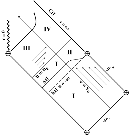
FIG. 1.: The Poisson-Israel spherical model of the black hole interior. The infalling wave-tail of gravitational radiation, and its scattered component, are modeled by lightlike dust. The region of purely ingoing (outgoing) dust is indicated by II (III) in the figure, and is described by a charged Vaidya solution. The solutions in regions II and III are matched to a Reissner-Nordström solution (region I) along the null rays $v=v_{0}$ and $u=u_{0}$. As usual ${\cal I}^{+}$ and ${\cal I}^{-}$ denote future and past null infinity. The inflow causes the apparent horizon (AH) to expand and smoothly approach the event horizon (EH) of the final black hole. The outflow in region IV causes the, initially static, Cauchy horizon (CH) to contract. This, together with the fatal blue shift experienced by the inflow, causes a curvature singularity to develop along CH.

In the limit as $v\rightarrow\infty$, the corresponding solution of Einstein’s equations is well approximated by

$$e^{\lambda} \simeq \frac{e^{-\kappa v}}{r}$$ (5)

$$r^{2} \simeq r_{\rm CH}^{2}+\frac{2\alpha(\kappa v)^{-q+1}}{\kappa^{2}(q-1)}-\frac{2\beta(-\kappa u)^{-q+1}}{\kappa^{2}(p-1)}\;,$$ (6)

where $r_{\rm CH}$ is the constant radius of the Cauchy horizon in region II. The square of the Weyl tensor diverges on the Cauchy horizon in this solution, yet the radial function given by Eq. (6) is non-zero for sufficiently large $|u|$. This indicates that the singularity is not a central ($r=0$) singularity with which we are familiar, in fact it is a null singularity. Spherical symmetry allows the introduction of a mass function $m(u,v)$ which is directly related to the Weyl curvature of the spacetime:

$$m(u,v) =\left(\mbox{$\textstyle\frac{1}{2}$}C{{}^{\theta\phi}}_{\theta\phi}r^{3}+q^{2}/r\right)$$ (8)

$$\stackrel{{\scriptstyle v\rightarrow\infty}}{{\longrightarrow}}\frac{\alpha\beta e^{\kappa v}}{\kappa r^{2}}(\kappa v)^{-q}(-\kappa u)^{-q}\;.$$

The divergence of this mass function as $v\rightarrow\infty$ in region IV prompted Poisson and Israel to refer to the accompanying scalar-curvature singularity as a mass inflation singularity.

Subsequently, Ori [4] pointed out that physical objects which encounter a mass-inflation singularity experience only finite tidal distortion, even though the tidal forces acting on the object diverge. In this sense, the mass-inflation singularities are weak although the relevance of this point continues to be debated [15, 16].

A variety of spherical models have now been studied [17, 18, 19], all of them indicate the presence of a null, scalar curvature singularity at the Cauchy horizon. The numerical analyses in [18] also demonstrates the slow contraction of the null generators of the Cauchy horizon to zero radius, and the formation of a spacelike singularity deep inside the black hole core.

B Beyond spherical symmetry

While simplified models argue strongly in favor of weak, null singularities inside black holes, the results are restricted entirely to spherical symmetry. Nevertheless the physics behind the mass-inflation phenomenon is extremely general. Perturbations originating in the external universe get infinitely blueshifted as they propagate close to the Cauchy horizon resulting in a scalar curvature singularity through non-linear interaction with gravity. Attempts have been made to investigate the problem in less symmetric situations. Ori [5] has used non-linear perturbation theory to examine back-reaction of perturbations on the Kerr geometry. His results support the existence of a weak, null singularity in this case. Bonanno [20] matched two radiating Kerr solutions along a null hypersurface and showed, in the limit of small angular momentum, that the mass-function diverges on a null hypersurface.

Brady and Chambers [21] demonstrated that weak, null singularities are consistent with the Einstein equations on a pair of intersecting null surfaces, and have investigated the rate of divergence of curvature on a null surface crossing the singularity. An important step has also been taken by Ori and Flanagan [22] who argue that the vacuum, Einstein equations admit functionally generic solutions containing weak, null singularities. Their results invalidate local arguments [23] that null singularities are always unstable to transformation into crushing spacelike singularities of the BKL type.

C Discussion and overview of this paper

In this paper we demonstrate that a null singularity replaces the Cauchy horizon inside a black hole formed by gravitational collapse. The method employed in the following analysis is similar in spirit to that of BKL [2]; we use an asymptotic expansion to find the leading order behavior of the metric near the Cauchy horizon without making any assumptions about the symmetry of the spacetime. In this way we show that the wave tail of gravitational collapse results in the formation of a null curvature singularity at the Cauchy horizon.

Our results should be compared with those obtained using non-linear perturbation theory. In that context, Ori [5] has previously argued that a weak, null singularity is present along the Cauchy horizon of a generic, rotating black hole. Our analysis, being asymptotic, relies on physical arguments to provide initial data near to the Cauchy horizon; in this sense, it is a local analysis. Nevertheless, the results presented below embody all orders of perturbation theory and lend further support to the claim that the perturbative approach captures the essential features of spacetime structure near the Cauchy horizon singularity inside a realistic, rotating black hole [5].

It is natural to use null coordinates to attack this problem since the Cauchy horizon is a null hypersurface. To facilitate the analysis we employ a double-null formalism [24] in which spacetime is decomposed into two families of intersecting null hypersurfaces. This decomposition of the Einstein field equations is reviewed in Sec. II where it is shown that the most general double-null metric depends on six functions of four variables. Interested readers are referred to Brady et al [24] for more details.

The main assumption made in this paper is that the results of scattering on the Kerr background [25] are sufficient to determine the initial data for the interior problem. This assumption and other physical considerations are discussed in Sec. III.

In Sec. IV we present the essential features of our arguments in a simplified context where the gravitational field has only one dynamical degree of freedom. We carefully construct the solution in the neighborhood of the Cauchy horizon for this model problem. Moreover, we demonstrate that the solution is characterized by a singularity at which the Weyl curvature diverges like

$$C_{\alpha\beta\gamma\delta}C^{\alpha\beta\gamma\delta}\sim v^{-(2l+3)}e^{2\kappa v}\ \ \$$ (9)

as $v\rightarrow\infty$ at the Cauchy horizon. We show that the resulting spacetime is not algebraically special except at the singularity, where it becomes asymptotically Petrov type N.

The relevance of the simplified model is made clear in Sec. V where we present the general analysis. By neglecting terms in the field equations which we expect to be exponentially small near to the Cauchy horizon, it is shown that the general solution is identical in character to that presented in Sec. IV.

Finally, we discuss the strength of the singularity in Sec. VI. While tidal forces experienced by an observer diverge at the singularity, the integrated tidal distortion is finite. As discussed by Ori [4, 5], the singularity is therefore weak and we are once again faced with the possibility that spacetime might extend beyond the Cauchy horizon (in a non-analytic manner). We emphasize that gravitational shock waves are the only type of curvature which can be confined to a thin layer in the absence of matter [15, 26]. This suggests that a classical continuation of spacetime beyond the Cauchy horizon is unlikely.

We adopt Misner, Thorne and Wheeler curvature conventions [27] with metric signature $(-+++)$ throughout the text. Greek indices $\alpha,\beta,\dots$ run from 0 to 3; upper-case Latin indices $A,B,\dots$ take values $(0,1)$; and lower-case Latin indices $a,b,\dots$ take values $(2,3)$.

II Double null formalism

The complexity of the Einstein equations requires the careful selection of a formalism with which to pursue our goal of understanding the nature of spacetime near null singularities. In [24] we have developed the necessary machinery based on a dual null decomposition of the Einstein field equations. In this section we present those details which are necessary for the application at hand. The interested reader is referred to [24] for a more complete treatment.

A Lightlike foliation of spacetime

We suppose that we are given a foliation of spacetime by lightlike hypersurfaces $\Sigma^{0}$ with normal generators $\ell^{(0)}$, and a second, independent foliation by lightlike hypersurfaces $\Sigma^{1}$ with generators $\ell^{(1)}$ nowhere parallel to $\ell^{(0)}$. The intersections of $\{\Sigma^{0}\}$ and $\{\Sigma^{1}\}$ define a foliation of codimension 2 by spacelike 2-surfaces $S$. (The topology of $S$ is unspecified. All our considerations are local.) $S$ has exactly two lightlike normals at each of its points, co-directed with $\ell^{(0)}$ and $\ell^{(1)}$.

In terms of local charts, the foliation is described by the embedding relations

$$x^{\alpha}=x^{\alpha}(u^{A},\theta^{a}).$$ (10)

Here, $x^{\alpha}$ are four-dimensional spacetime co-ordinates; $u^{0}=v$ and $u^{1}=u$ are a pair of scalar fields constant over each of the hypersurfaces $\Sigma^{0}$ and $\Sigma^{1}$ respectively. The intrinsic co-ordinates $\theta^{a}$ of the 2-spaces $S$, each characterized by a fixed pair of values $(u^{0},u^{1})$, are convected along the vectors $\partial/\partial u^{A}$.

It is convenient to effect a partial normalization of the lightlike vectors $\ell^{(A)}$ by imposing the condition

$${}^{(4)}g^{\alpha\beta}\ell^{(A)}_{\alpha}\ell^{(B)}_{\beta}=e^{\lambda}\eta^{AB}\equiv e^{\lambda}\,\mbox{\rm anti-diag}\,(-1,-1)$$ (11)

for some scalar field $\lambda(x^{\alpha})$, reflecting the freedom to arbitrarily rescale a null vector. The superscript $(4)$ is used to indicate four dimensional objects whenever confusion might arise. We can use $\eta^{AB}$ and its inverse $\eta_{AB}$ to raise and lower uppercase Latin indices. Furthermore, the vectors $\ell^{(A)}$ are parallel to the gradients of $u^{A}$ allowing us to write

$$\ell^{(A)}_{\alpha}=e^{\lambda}\partial_{\alpha}u^{A}\;.$$ (12)

The pair of vectors $e_{(a)}^{\alpha}$, defined from (10) by

$$e_{(a)}^{\alpha}=\partial x^{\alpha}/\partial\theta^{a},$$ (13)

are holonomic basis vectors tangent to $S$. The intrinsic metric $g_{ab}$ of $S$ is determined by their scalar products:

$$g_{ab}={}^{(4)}g_{\alpha\beta}e_{(a)}^{\alpha}e_{(b)}^{\beta}.$$ (14)

Lower-case Latin indices are lowered and raised with $g_{ab}$ and its inverse $g^{ab}$. Since $\ell^{(A)}$ is normal to every vector in $\Sigma^{A}$, we have

$$\ell^{(A)}_{\alpha}e_{(a)}^{\alpha}=0.$$ (15)

Finally, introducing a pair of shift vectors $s_{A}^{\alpha}$ tangent to $S$ by

$$\frac{\partial x^{\alpha}}{\partial u^{A}}=\ell_{(A)}^{\alpha}+s_{A}^{a}\,e_{(a)}^{\alpha}\;,$$ (16)

an arbitrary displacement $dx^{\alpha}$ in spacetime is

$$dx^{\alpha}=\ell^{\alpha}_{(A)}du^{A}+e^{\alpha}_{(a)}(d\theta^{a}+s^{a}_{A}du^{A})\;.$$ (17)

Thus, the final form of the line element used below to discuss the black hole interior is

$$ds^{2}=e^{\lambda}\eta_{AB}\,du^{A}\,du^{B}+g_{ab}(d\theta^{a}+s_{A}^{a}\,du^{A})(d\theta^{b}+s_{B}^{b}\,du^{B}).$$ (18)

We will impose further coordinate conditions as the need arises, but it is manifest that Eq. (2.9) is sufficient to describe the most general spacetime admitted as a solution to the Einstein field equations.

B 2+2 decomposition of curvature

Following [24], the components of the Ricci tensor can be compactly expressed in terms of two dimensionally covariant quantities. In passing to these expression we must first introduce some notation. The extrinsic curvatures of $S$ are defined by

$$2K_{Aab} \equiv e^{\alpha}_{(a)}e^{\beta}_{(b)}\left[{{}^{(4)}\mbox{$\cal L$}_{\ell_{(A)}}}\bar{g}_{\alpha\beta}\right]$$ (19)

$$= D_{A}g_{ab}\;,$$ (20)

where $\bar{g}_{\alpha\beta}={}^{(4)}g_{\alpha\beta}-e^{\lambda}\eta_{AB}\ell^{(A)}_{\alpha}\ell^{(B)}_{\beta}=e^{(a)}_{\alpha}e^{(b)}_{\beta}g_{ab}$ is the spatial projection tensor, and ${{}^{(4)}\mbox{$\cal L$}_{\ell_{(A)}}}$ is the four dimensional Lie derivative along $\ell_{(A)}$. We have also introduced the derivative operators $D_{A}$ acting on two-dimensional tensorial objects according to the rule

$$D_{A}X{{}^{a\ldots}}_{b\ldots}=(\partial_{A}-\mbox{$\cal L$}_{s^{d}_{A}})X{{}^{a\ldots}}_{b\ldots}\;.$$ (21)

Here $\mbox{$\cal L$}_{s^{d}_{A}}$ is the two-dimensional Lie derivative. (Generally $D_{A}$ can be defined in a four-dimensionally covariant manner by its action on spatial four tensors [24];

$$D_{A}X{{}^{a\ldots}}_{b\ldots}\equiv e^{(a)}_{\alpha}e_{(b)}^{\beta}{{}^{(4)}\mbox{$\cal L$}_{\ell_{(A)}}}(X{{}^{c\ldots}}_{d\ldots}e^{\alpha}_{(c)}e^{(d)}_{\beta})\;,$$ (22)

thus providing a complete geometrical interpretation of $D_{A}$ in terms of Lie derivatives.)

The geometric meaning of the extrinsic curvature is illustrated by Lie propagating a circle on $S$ along $\ell_{(A)}$. The expansion rate of the light rays is given by the trace of the extrinsic curvature $K_{A}\equiv g^{ab}K_{Aab}$. The traceless part of the extrinsic curvature, $\sigma_{Aab}\equiv K_{Aab}-\mbox{$\textstyle\frac{1}{2}$}g_{ab}K_{A}$, is the shear of the null congruence, and the twist is

$$\omega^{\alpha} \equiv [\ell_{(1)},\ell_{(0)}]^{\alpha}$$ (23)

$$= e^{\alpha}_{(a)}\epsilon^{AB}(\partial_{B}s^{a}_{A}-s^{b}_{B}\partial_{b}s^{a}_{A})$$ (24)

where $\epsilon_{AB}$ is the anti-symmetric tensor density ($\epsilon_{01}=1$). Clearly $\omega^{\alpha}$ is purely spatial.

Finally, the expressions for the Ricci tensor are [

$${}^{(4)}\!R_{ab}=R_{\alpha\beta}e_{(a)}^{\alpha}e_{(b)}^{\beta} = -\mbox{$\textstyle\frac{1}{2}$}g_{ab}e^{-\lambda}(D_{A}K^{A}+K_{A}K^{A})+e^{-\lambda}(-D^{A}\sigma_{Aab}+2\sigma{{}_{A(a}}^{d}\sigma{{}^{A}}_{b)d})$$ (26)

$$+\frac{1}{2}\,^{(2)}\!Rg_{ab}-\frac{1}{2}e^{-2\lambda}\,{\omega_{a}\omega_{b}}-\lambda_{;ab}-\frac{1}{2}\lambda_{,a}\lambda_{,b}$$

$$R_{AB}=R_{\alpha\beta}\ell_{(A)}^{\alpha}\ell_{(B)}^{\beta} = -D_{(A}K_{B)}-\mbox{$\textstyle\frac{1}{2}$}K_{A}K_{B}-\sigma_{Aab}\sigma_{B}\,^{ab}+K_{(A}D_{B)}\lambda$$ (28)

$$\qquad-\frac{1}{2}\eta_{AB}\left[\left(D^{E}+K^{E}\right)D_{E}\lambda-e^{-\lambda}\omega^{a}\omega_{a}+(e^{\lambda}){{}^{;a}}_{;a}\right]$$

$$R_{Aa}=R_{\alpha\beta}e_{(a)}^{\alpha}\ell_{(A)}^{\beta} = \sigma{{{}_{Aa}}^{b}}_{;b}-\mbox{$\textstyle\frac{1}{2}$}\partial_{a}K_{A}-\frac{1}{2}\partial_{a}D_{A}\lambda+\frac{1}{2}K_{A}\partial_{a}\lambda$$ (30)

$$\qquad+\frac{1}{2}\epsilon_{AB}e^{-\lambda}\left[\left(D^{B}+K^{B}\right)\omega_{a}-\omega_{a}D^{B}\lambda\right],$$

]

where ${}^{(2)}\!R$ is the curvature scalar associated with the two-metric $g_{ab}$, and a semi-colon indicates the two-dimensional covariant derivative.

III Assumptions

The mathematical theory of black holes is well established [28]. Indeed, it is widely accepted that the external geometry of a black hole formed by the gravitational collapse of a star is described by a Kerr-Newman solution at late times. The mechanism by which the black hole settles down to this stationary state was elucidated by Price [8] for nearly spherical, uncharged collapse, and his results have been extended to other situations by several authors [9, 29]. These works provide the initial conditions for the interior problem by determining the behavior of the radiative tail of gravitational waves at the event horizon of the black hole: in particular, the amplitude of the gravitational wave flux generally decays as an inverse power of advanced time.

Some simplifying assumptions are required in order to make progress against the black-hole interior problem. We clarify our approach below.

A Physical considerations

The inner Cauchy horizon of a stationary black hole is unstable to linear perturbations that undergo infinite gravitational blueshift there. The central assumption of our analysis is that an asymptotic limit exists in which effects on the geometry, inside a black hole formed by gravitational collapse, are dominated by gravitationally blueshifted tail-radiation which propagates into the black hole at late times (as measured by external observers). The postulated structure of spacetime inside the black hole is shown in Fig. 2. On physical grounds [30] one expects that the region between the event horizon and the three dimensional spacelike surface $\Sigma$ can be adequately described by linear perturbation theory—there is no physical mechanism to excite an instability of the interior before the blueshifting takes hold. We examine the structure of spacetime in the region to the future of $\Sigma$ and near to the Cauchy horizon, given initial data consistent with scattering of a test gravitational wave field inside a Kerr black hole [25].

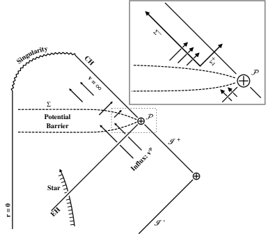
FIG. 2.: A schematic representation of the spacetime structure of a realistic black hole formed by the collapse of a rotating star. An observer falling in with the surface of the star encounters a spacelike singularity indicated by the zig-zag line in the figure. Gravitational radiation, originating from the stellar collapse, gets partially scattered into the black hole; at late times, this flux decays as an inverse power of external advanced time $v^{-q}$. The radiation which crosses the event horizon (EH) gets scattered once again by the inner gravitational potential barrier (indicated in the figure). The result is a flux of gravitational waves irradiating the Cauchy horizon (CH) and causing it to contract. Note that CH is located at $v=\infty$ in these coordinates. The inset shows the set up of the characteristic initial value problem solved in the text. The two initial characteristics $\Sigma^{+}$: $u=u_{0}$ and $\Sigma^{-}$: $v=v_{0}$ are indicated. The shear along these characteristic surfaces has an inverse power-law dependence on the advanced and retarded times reflecting the behavior of the late time wave tail of gravitational collapse.

The late-time wave tail of gravitational collapse produces a flux of radiation across the black-hole event horizon which decays as an inverse power-law of external advanced time [29]. Starting from these initial conditions Ori [25] has examined the scattering of a test field inside a Kerr black hole. His results indicate that the amplitudes of test fields decay as an inverse power-law in both retarded and advanced times $u$ and $v$ near to $\cal P$ in Fig. 2. Ori also argues that the decay of non-axisymmetric modes is modulated by oscillatory terms which originate from the rotation of the inner horizon with respect to infinity, i.e. the oscillations are a direct consequence of frame dragging in the Kerr geometry. Since these oscillations have no counterpart in spherical symmetry it seems worthwhile to outline Ori’s argument here.

The line element for the Kerr spacetime, written in familiar Boyer-Lindquist coordinates, is

$$ds^{2} = -(1-2Mr/\rho^{2})dt^{2}+(\rho^{2}/\Delta)dr^{2}+\rho^{2}d\theta^{2}$$ (33)

$$+[r^{2}+a^{2}+(2Mra^{2}/\rho^{2})\sin^{2}\theta]\sin^{2}\theta d\phi^{2}$$

$$-(4Mra/\rho^{2})\sin^{2}\theta d\phi dt\;,$$

where $\rho^{2}=r^{2}+a^{2}\cos^{2}\theta$ and $\Delta=r^{2}-2Mr+a^{2}$. The solution depends on two parameters: the mass $M$, and the angular momentum per unit mass $a$. The equations governing perturbations of the Kerr spacetime are not fully separable in coordinate space, this indicates that the evolution of various multipoles are coupled. However, Ori argues that the coupling between multipoles should be weak at late times so that a good first approximation to the fields can be obtained by decomposing them over the spherical harmonics, and solving the resulting equations while neglecting the coupling completely. One then iterates to obtain better approximations to the solutions. At late times, on a surface of constant coordinate $r$ outside the event horizon, the field is given approximately by

$$\Psi_{lm}\simeq F(r,\theta)e^{im\phi}t^{-(2l+2)}\;,$$ (34)

where $l\geq|m|$, and $F$ is some function of both $r$ and $\theta$. The time dependence of this result has been verified numerically by Krivan et al[31]. Now, the coordinate $\phi$ is badly behaved at the black hole event horizon. When the field is expressed in terms of the regular coordinate $\phi_{+}=\phi-\Omega_{+}t$, where $\Omega_{+}=a/(2Mr_{+})$, and matched to the ingoing solution at the event horizon $r=r_{+}$, one arrives at

$$\Psi_{lm}\simeq F_{+}(\theta)e^{im\phi_{+}}e^{im\Omega_{+}v}v^{-(2l+2)}\;.$$ (35)

In the final step, this ingoing solution gets matched to the solution near to the Cauchy horizon (denoted by $r_{-}$) giving the final expression

$$\Psi_{lm}\simeq\left[F_{v}(\theta)e^{im\Omega_{-}v}v^{-(2l+2)}+F_{u}(\theta)e^{im\Omega_{-}u}u^{-(2l+2)}\right]e^{im\phi_{-}}\;.$$ (36)

Here $F_{u}$ and $F_{v}$ are functions to be determined, and $\phi_{-}=\phi-\Omega_{-}t$. The source of the oscillations in the non-axisymmetric modes is now obvious.

While this argument seems plausible, it is far from rigorous. In order to assess the complete significance of these non-axisymmetric modes it would be necessary to establish the amplitudes of these terms at late times, information which is currently unavailable. For this reason we focus our attention on the power-law decay of the wave tail; however, we do indicate where these oscillations might modify the analysis.

B Coordinate conditions

While the conclusions of our analysis are couched in terms of physical observables, such as the tidal forces (and distortion) experienced by observers approaching the singularity inside a black hole, or in terms of curvature scalars, it is extremely important to understand the coordinates used to describe the spacetime.

The Cauchy horizon can be thought of as the extension of future null infinity inside the black hole; that is, the Cauchy horizon is located at infinite external advanced time. Therefore it is convenient to fix the coordinate $v$ to be standard, external advanced time as measured by an observer far outside the black hole. Since the external geometry settles down to a stationary state at late times, and the strength of the tail radiation crossing the black hole horizon decays, we assume that $e^{\lambda}\sim e^{-\kappa v}$ as $v\rightarrow\infty$; this is known to hold in non-linear evolution of scalar fields in the spherical case, and is the coordinate expression of the infinite gravitational blueshift between the external universe and the Cauchy horizon. In the subsequent analysis we will show that this assumption leads to a self-consistent picture of the black-hole interior. The approach adopted here is similar in spirit to that of BKL [2]; we neglect terms in the field equations which are suppressed by the exponential factor $e^{\lambda}$ and solve the resulting asymptotic equations.

The coordinate $u$ is chosen so that it goes to negative infinity at the event horizon of the black hole. In this way, it can be taken to coincide with the natural retarded time coordinate inside a Kerr black hole at late times.

Finally, the coordinates $\theta^{a}$ on the two surfaces of foliation will be fixed as required by the analysis.

IV A simplified model—almost plane symmetry

The goal of the present work is to examine the structure of spacetime in the neighborhood of the Cauchy horizon of a black hole formed by the collapse of a rotating star. The essential features of our analysis are most clearly illustrated in a slightly simplified context where the Cauchy horizon is irradiated by gravitational waves of a single polarization—this interpretation is motivated by the local “almost plane symmetry” of the spacetime we consider below.

In this section we set $s_{A}\equiv 0$, writing the line element as

$$ds^{2}=-2e^{\lambda}dudv+\rho^{2}h_{ab}d\theta^{a}d\theta^{b}\;,$$ (37)

where we allow the remaining metric functions $\rho^{2}$, $\lambda$ and $h_{ab}$ to depend on all the coordinates $\{u,v,\theta^{a}\}$. In addition, we assume that one may simultaneously choose coordinates in which the conformal metric $h_{ab}$ is diagonal, and write

$$h_{ab}d\theta^{a}d\theta^{b}=e^{-2\beta}dx^{2}+e^{2\beta}dy^{2}\;.$$ (38)

The assumption of vanishing shift vectors reduces the Lie derivative operators $D_{A}$ to simple partial derivatives, i.e. $D_{A}=\partial_{A}$. As a result, the shear tensor has the simple form

$$\sigma_{Aab}=\rho^{2}\beta_{,A}{\rm diag}[-e^{-2\beta},e^{2\beta}]\;,$$ (39)

where a comma indicates partial differentiation. Similarly, the expansion rates of the null rays orthogonal to the surfaces $S$ are simply $K_{A}=2\rho^{-1}\rho_{,A}$, and the twist, given by Eq. (24), vanishes identically.

These additional assumptions reduce the Eqs. (26)-(30) to a manageable form in which the central features of our arguments are easily understood. Moreover, relaxing these conditions in Sec. V results in equations which are sufficiently similar in structure that only slight modification of the following arguments are required to complete the general analysis.

A The asymptotic form of the equations

In the coordinates described above, the asymptotic regime of interest is characterized by the exponentially small value of $e^{\lambda}$. This is so because we have tailored our coordinates to the physical mechanism which underlies the Cauchy horizon instability—the gravitational blueshift. Moreover, the vacuum Einstein equations (26)–(30) reduce to

$$-D_{(A}K_{B)}-\mbox{$\textstyle\frac{1}{2}$}K_{A}K_{B}-\sigma_{Aab}\sigma_{B}\,^{ab}\mbox{\hskip 21.68121pt}$$ (40)

$$+K_{(A}D_{B)}\lambda-\frac{1}{2}\eta_{AB}\left(D^{E}+K^{E}\right)D_{E}\lambda \simeq 0$$ (41)

$$-\mbox{$\textstyle\frac{1}{2}$}\rho^{2}h_{ab}(D_{A}K^{A}+K_{A}K^{A})\mbox{\hskip 36.135pt}$$ (42)

$$-D^{A}\sigma_{Aab}+2\sigma_{A(a}^{\;\;\;d}\sigma_{b)d}^{A} \simeq 0$$ (43)

and

$$\sigma_{Aa;b}^{\;b}-\mbox{$\textstyle\frac{1}{2}$}\partial_{a}K_{A}-\frac{1}{2}\partial_{a}D_{A}\lambda+\frac{1}{2}K_{A}\partial_{a}\lambda\simeq 0\;,$$ (44)

where we have discarded terms in the equations which are damped by a pre-factor $e^{\lambda}$.

In the following argument Eq. (44) constrains the dependence of each of the dynamical variables on $\theta^{a}$ near to the Cauchy horizon; it can be ignored until later. Contracting Eq. (43) with $h^{ab}$ and substituting for $K_{A}$ and $D_{A}$ gives

$$(\rho^{2})_{,uv}\simeq 0$$ (45)

which is readily solved for $\rho^{2}$:

$$\rho^{2}\simeq\rho^{2}_{0}(\theta^{a})+L(v,\theta^{a})+R(u,\theta^{a})\;.$$ (46)

Here $\rho_{0}(\theta^{a})$ is assumed to be non-vanishing almost everywhere. The functions $L(v,\theta^{a})$ and $R(u,\theta^{a})$ are determined by the initial data. The precise form depends on the detailed evolution of the gravitational field between the event horizon and $\Sigma$; we make some minimal assumptions below.

Substituting Eq. (45) into Eq. (43) provides a simple equation for the shear, which can be expanded to a second order equation for $\beta$ as

$$\rho\beta_{,uv}+\rho_{,u}\beta_{,v}+\rho_{,v}\beta_{,u}\simeq 0\;.$$ (47)

Defining a function $\Lambda$ by

$$\Lambda=\lambda+\ln\rho\;,$$ (48)

and contracting Eq. (41) with $\eta_{AB}$ gives

$$\Lambda_{,uv}\simeq-\sigma_{uab}\sigma{{}_{v}^{ab}}\;,$$ (49)

where the inhomogeneous term $\sigma_{uab}\sigma_{v}{{}^{ab}}=2\beta_{,u}\beta_{,v}$ for the metric in Eq. (38)

B Initial conditions

Initial data for Eqs. (41)-(44) is provided on a pair of characteristic surfaces, one of which crosses the Cauchy horizon as shown in Fig. 2. This is not completely satisfactory, as it assumes the existence of the Cauchy horizon, at least on one initial characteristic surface. Ideally we would like to place initial data on a spacelike surface, such as $\Sigma$, below the inner potential barrier, but on the past boundary of the region of high blueshift. Unfortunately, this program is impractical in the present context. Instead we insure that the solution we construct is consistent with such initial data—the solution could be smoothly matched to that of a stationary black hole background with small perturbations.

The choice of external advanced time $v$ to describe spacetime near the Cauchy horizon implies that $e^{\lambda}\rightarrow 0$ on the Cauchy horizon. In particular, on the initial characteristic surface $\Sigma^{+}$ ($u=u_{0}$) we write

$$\Lambda|_{+}\simeq\Lambda_{0}(\theta^{a})-\kappa(v-v_{0})+\ldots$$ (50)

where $\Lambda_{0}(\theta^{a})$ is its value on the two surface $S^{0}=\{\Sigma^{+}\cap\Sigma^{-}\}$, $\kappa$ is a constant with the dimension of inverse length, and terms which vanish in the limit of $v\rightarrow\infty$ are indicated by dots. A similar condition is demanded on $\Sigma^{-}$ ($v=v_{0}$):

$$\Lambda|_{-}\simeq\Lambda_{0}(\theta^{a})-\kappa(u-u_{0})+\ldots\;.$$ (51)

Up to the surface $\Sigma$ on which effects of gravitational blueshifting begin to take hold, the evolution of the decaying wave tail of gravitational collapse is well described by perturbation theory. To the future of this surface the large blueshift suggests that geometric optics is valid, and that ingoing gravitational waves will be negligibly scattered by the gravitational field. Consistent with this picture we write the initial data for the shear as

$$\beta_{,v}|_{+} \simeq (\kappa v)^{-q/2}[\mu(\theta^{a})+\ldots]\;,$$ (52)

$$\beta_{,u}|_{-} \simeq (-\kappa u)^{-p/2}[\nu(\theta^{a})+\ldots]\;,$$ (53)

where $\mu(\theta^{a})$ and $\nu(\theta^{a})$ are unspecified functions on the two surfaces which foliate the two initial characteristic hypersurfaces. The inverse power-law decay is motivated by the behavior of the tail radiation crossing the event horizon of the black hole. The precise nature of the outflux is irrelevant, although it must decay sufficiently fast as $u\rightarrow-\infty$ [14]. While perturbation theory suggests that $p=q$, we allow for more general behavior. The qualitative picture which emerges below remains unchanged provided $\beta_{,v}|_{+}$ decays at least as fast as $v^{-3/2}$ but not faster than $e^{-\kappa v}$. In particular, oscillatory terms which modulate the power-law decay, due to differential rotation of the event horizon and the Cauchy horizon of a rotating black hole, do not change the important features of the analysis below. These oscillatory terms will show up as the higher order corrections in Eqs. (52) and (53).

Using Eqs. (52) and (53) we can now solve Raychauduri’s equation for $\rho^{2}$ on $\Sigma^{+}$ (obtained from Eq. (41) by setting $B=A=v$)

$$(\rho^{2})_{,vv}-(\rho^{2})_{,v}\,\partial_{v}\Lambda=-2\rho^{2}(\beta_{,v})^{2}\;.$$ (54)

This determines the function $L(v,\theta^{a})$, which can be written as

$$L(v,\theta^{a})\simeq(\kappa v)^{-q+1}\frac{2[\rho_{0}\mu(\theta^{a})]^{2}}{\kappa^{2}(q-1)}\left[1+O(1/v)\right]$$ (55)

in the large $v$ limit. The explicit form of $R(u,\theta^{a})$ is unnecessary. It is sufficient to note that $\partial_{u}R(u,\theta^{a})\rightarrow 0$ as $u\rightarrow-\infty$.

With this information, it is straightforward to check that the curvature diverges as $v\rightarrow\infty$ along $\Sigma^{+}$, and that the behavior is consistent with the discussion in Brady and Chambers [21].

C The evolution

We now examine the solution determined by the initial data constructed in the previous section. The evolution of the gravitational degrees of freedom (the conformal two-metric $h_{ab}$) is dictated by the linear wave Eq. (47). Therefore the crucial step in determining the geometry of spacetime near the Cauchy horizon is to understand the evolution of $\beta$ from which the gravitational shear is directly determined. If $\beta$ was to diverge the assumptions stated in Sec. III would be violated, and our entire analysis would break down.

In this almost plane symmetric model, we can construct an explicit solution of Eq. (47) and demonstrate that $\beta$ remains finite, and use it to show that $e^{-\Lambda}\rightarrow 0$ on the Cauchy horizon for a finite range of $u$. For the general case presented in Sec. V we are not afforded the luxury of an exact solution, therefore we also present a method which provides a useful bound on the shear near to the Cauchy horizon singularity and is applicable in the general case.

The linearity of Eq. (47) makes it directly amenable to Fourier techniques (see Appendix A), however it is more illuminating to write the solution as a series

$$\beta=\beta_{0}+\rho^{-1}\sum_{i\geq 0}A_{i}\rho^{-2i}\left[F^{(-i)}(V)+G^{(-i)}(U)\right]$$ (56)

where $V=L(v,\theta^{a})$, and $U=R(u,\theta^{a})$. The notation $F^{(-i)}$ indicates the $i$-th integral of the function $F(x)\equiv F^{(0)}(x)$ with respect to $x$. Inserting (56) into Eq. (53) and comparing integrals of the same order gives the coefficients

$$A_{i+1}=A_{i}\frac{(2i+1)^{2}}{4(i+1)}.$$ (57)

The functions $F(V)$, $G(U)$ and $A_{0}(\theta^{a})$ are determined by the initial data.

Differentiating Eq. (56) with respect to $v$ and comparing with the initial data along $\Sigma^{+}$ determines $F$ in the limit $v\rightarrow\infty$ to be given by

$$F^{(1)}\,\partial_{v}L(v,\theta^{a})\simeq\frac{\rho_{0}\,(\kappa v)^{-q/2}}{2A_{0}}[\mu(\theta^{a})+\ldots]\;,$$ (58)

from which one can extract the behavior of $F$ to be

$$F(v,\theta)\simeq\frac{\rho_{0}\,(\kappa v)^{1-q/2}}{A_{0}\kappa(2-q)}[\mu(\theta^{a})+\ldots]\;.$$ (59)

Given the solution (59) and $L(v,\theta^{a})$ in Eq. (55) one derives the recursion relation

$$F^{(-i-1)}=F^{(-i)}\frac{(\kappa v)^{1-q}}{(i+1)(1-q)+1-q/2}\;.$$ (60)

Combining Eqs. (60), (59) and (57) it is easy to check that the sum over $F^{(-i)}$ converges to a finite result provided $q>3$—the boundary conditions for the radiative tail at the event horizon actually imply $q\geq 14$.

It follows that the leading order term in Eq. (56) is proportional to $F$ since $F^{(-i)}(V)\gg F^{(-i-1)}(V)$ for large $v$. This shows that $\beta_{,v}$ continues to decay with an inverse power-law form all along the Cauchy horizon provided it has such a decay on the initial surface. Similar arguments provide $G$.

We can now use Eq. (56) to compute the source term in Eq. (49) and hence determine the evolution of $\Lambda$ to be

$$\Lambda\simeq\Lambda|_{-}(u,\theta^{a})-\kappa(v-v_{0})-\int_{u_{0}}^{u}\!du^{\prime}\int_{v_{0}}^{v}dv^{\prime}\sigma_{uab}\sigma{{}_{v}}^{ab}\;.$$ (61)

The integrand in Eq. (61) is proportional to $\beta_{,u}\beta_{,v}\sim(\kappa v)^{-q/2}$ as $v\rightarrow\infty$, consequently the integral is finite in this limit provided $q>2$ as we have already required. Clearly, $\Lambda$ diverges to negative infinity at the Cauchy horizon in precisely the same manner as it does along the initial hypersurface $\Sigma^{+}$, that is

$$\Lambda\sim-\kappa v$$ (62)

as $v\rightarrow\infty$. Equation (44) provides a final consistency check on the solution.

Having determined the approximate solution to Eqs. (41)-(44) near to the Cauchy horizon we are in a position to examine the curvature. It is convenient to consider the Newman-Penrose components of the Weyl tensor on the basis

$$\{e^{-\lambda/2}\ell_{(0)},e^{-\lambda/2}\ell_{(1)},e_{(a)}m^{a},e_{(a)}\bar{m}^{a}\}\;,$$ (63)

where $m^{a}$ is a complex two-vector (called the shear axis) which satisfies $g_{ab}=2m_{(a}\bar{m}_{b)}$. The leading behavior of each of the Weyl scalars is presented below:

$$\Psi_{0} =e^{-\lambda}(\kappa v)^{-\frac{q}{2}}[-\kappa\mu(\theta^{a})+\ldots]$$ (64)

$$\Psi_{1} =-e^{-\frac{\lambda}{2}}(\kappa v)^{-\frac{q}{2}}[m^{a}\partial_{a}(\mu\nu)(-\kappa u)^{-\frac{p}{2}+1}+\ldots]$$ (65)

$$\Psi_{2} =e^{-\lambda}(\kappa v)^{-\frac{q}{2}}[-\mu(\theta^{a})\nu(\theta^{a})(-\kappa u)^{-\frac{p}{2}}+\ldots]$$ (66)

$$\Psi_{3} =e^{-\frac{\lambda}{2}}(\kappa v)^{-\frac{q}{2}+1}[\bar{m}^{a}\partial_{a}(\mu\nu)(-\kappa u)^{-\frac{p}{2}}+\ldots]$$ (67)

$$\Psi_{4} =e^{-\lambda}(-\kappa u)^{-\frac{p}{2}}[-\kappa\nu(\theta^{a})+\ldots].$$ (68)

Notice that $\Psi_{1}$ and $\Psi_{3}$ are non-zero, this arises because the spacetime is not exactly plane symmetric. The square of the Weyl curvature $C_{\alpha\beta\gamma\delta}C^{\alpha\beta\gamma\delta}$ diverges as $v\rightarrow\infty$ at the Cauchy horizon, and is dominated by the radiative piece $\Psi_{0}\Psi_{4}$ on this tetrad. Degeneracy of the roots of the polynomial

$$a^{4}\Psi_{4}+a^{3}\Psi_{3}+a^{2}\Psi_{2}+a\Psi_{1}+\Psi_{0}=0$$ (69)

determines the Petrov classification of the spacetime [28]. Brady and Chambers [21] demonstrated a four-fold degeneracy in the limit that $v\rightarrow\infty$ on $\Sigma^{+}$. Using Eqs. (66) one shows that this statement continues to hold near to the Cauchy horizon but away from $\Sigma^{+}$, that is, the diverging curvature is asymptotically Petrov type N. This suggests the intuitive physical picture of the singularity as a gravitational shock wave propagating along the Cauchy horizon. It is worth noting however that this approach to type N behavior is not characterized by a peeling property as it is at large distances outside the black hole. Indeed $a^{2}\rightarrow\pm\sqrt{-4\Psi_{0}/\Psi_{4}}$ as $v\rightarrow\infty$ so that all four roots tend to zero. This behavior is indicated schematically in Fig 3.

FIG. 3.: The complex plane showing a schematic representation of the roots of Eq. (69). The arrows indicate the evolution of the roots as $v\rightarrow\infty$. The roots become degenerate in the asymptotic limit, but they do not exhibit any peeling like properties. This suggests that the Cauchy horizon singularity is Petrov Type N, and can be thought of intuitively as a shock wave propagating into the black hole.

D Alternative bounds

The most important step in validating the approximation adopted in this paper is to show that $e^{\Lambda}\rightarrow 0$ as $v\rightarrow\infty$ everywhere along the Cauchy horizon. In the simple model spacetime examined above, we have the explicit solution (56) for the metric function $\beta$ which determines the shear tensors through (39). Once the shear tensors are known, the evolution of $\Lambda$ is given by the integral equation (61). The linearity of the wave equation (47) allows the direct computation of $\beta$, and the explicit verification that the integral appearing in Eq. (61) vanishes in the limit $v\rightarrow\infty$.

In a general spacetime, the evolution of the shear tensors are described by a non-linear wave equation for which no exact solution is known. However, it is still possible to place bounds on the integral appearing in Eq. (61) by using the field equations, thus verifying that $e^{\Lambda}\rightarrow 0$ as $v\rightarrow\infty$. Although this procedure is unnecessary here, it is instructive to apply it first to this case before considering the general non-linear problem in the succeeding section.

First define a new function $\xi$ which is proportional to the integrand,

$$\xi(u,v,\theta^{a})=2\beta_{,u}\beta_{,v}\;.$$ (70)

Multiplying the wave Eq (47) for $\beta$ by $\beta_{,v}$, it is not difficult to derive

$$\partial_{u}\left[\rho^{2}(\beta_{,v})^{2}\right]=-\frac{1}{2}(\rho^{2})_{,v}\xi.$$ (71)

Integrating (71) with respect to $u$, making use of the characteristic initial data (52) and the solution (55) for the $v$ dependence of $\rho^{2}$, we find

$$(\beta_{,v})^{2}=\frac{[\mu(\theta^{a})\rho_{0}(\theta^{a})]^{2}(\kappa v)^{-q}}{\kappa\rho^{2}(u,v,\theta^{a})}\left(\kappa+\int_{u_{0}}^{u}\xi du\right)$$ (72)

for $u>u_{0}$.

Suppose that at a point with coordinates $\bar{u}$, $\bar{v}$ where $\bar{u}\in[u_{0},u]$ and $\bar{v}\in[v_{0},v]$, the largest value of the function $\xi$ occurs such that $\xi(\bar{u},\bar{v})=\bar{\xi}$. We denote the value of any function evaluated at this point with an overbar. The partial derivative of $\beta$ evaluated at this point is bounded by

$$\bar{\beta}^{2}_{,v}\leq\frac{[\mu(\theta^{a})\rho_{0}(\theta^{a})]^{2}(\kappa\bar{v})^{-q}}{\kappa\bar{\rho}^{2}}\left(\kappa+(\bar{u}-u_{0})\bar{\xi}\right).$$ (73)

A similar bound on the square of the partial derivative of $\beta$ with respect to $u$ can be derived,

$$\bar{\beta}^{2}_{,u}\leq\frac{[\nu(\theta^{a})\rho_{0}(\theta^{a})]^{2}(-\kappa\bar{u})^{-p}}{\kappa\bar{\rho}^{2}}\left(\kappa+(\bar{v}-v_{0})\bar{\xi}\right).$$ (74)

It then follows from these bounds and from the definition of $\bar{\xi}$ that the inequality

$$\bar{\xi}^{2} = 4\bar{\beta}^{2}_{,v}\bar{\beta}^{2}_{,u}$$ (75)

$$\leq 4\left(\frac{\mu\nu\rho_{0}^{2}}{\kappa\bar{\rho}^{2}}\right)^{2}(\kappa\bar{v})^{-q}(-\kappa\bar{u})^{-p}\left(\kappa+(\bar{u}-u_{0})\bar{\xi}\right)$$ (77)

$$\mbox{\hskip 72.26999pt}\times\left(\kappa+(\bar{v}-v_{0})\bar{\xi}\right)$$

must be satisfied if the field equations are satisfied. This inequality can be rearranged into the form

$$a\bar{\xi}^{2}-b\bar{\xi}-c\leq 0$$ (78)

where the coefficients are given by

$$a\! = \!1-4\left(\frac{\mu\nu\rho_{0}^{2}}{\kappa\bar{\rho}^{2}}\right)^{2}(\kappa\bar{v})^{-q}(-\kappa\bar{u})^{-p}(\bar{u}-u_{0})(\bar{v}-v_{0})$$ (79)

$$b\! = \!4\kappa\left(\frac{\mu\nu\rho_{0}^{2}}{\kappa\bar{\rho}^{2}}\right)^{2}(\kappa\bar{v})^{-q}(-\kappa\bar{u})^{-p}\left(\bar{u}\!-\!u_{0}\!+\!\bar{v}\!-\!v_{0}\right)\!\geq\!0$$ (80)

$$c\! = \!4\kappa^{2}\left(\frac{\mu\nu\rho_{0}^{2}}{\kappa\bar{\rho}^{2}}\right)^{2}(\kappa\bar{v})^{-q}(-\kappa\bar{u})^{-p}\geq 0.$$ (81)

Clearly, if the coefficient $a$ in this inequality is negative, then no bound can be placed on the maximum value of $\xi$. However, if $a$ is positive, then the upper bound on $\bar{\xi}$ is just given by $\bar{\xi}\leq b/2a+(b^{2}+4ac)^{1/2}/2a$. Hence, it is important to determine the sign of the coefficient $a$, which will depend on the relative magnitudes of the two contributions to $a$.

Now, consider the magnitude of the second term in (79). At a fixed value of $\bar{u}$, this term is proportional to $(\kappa\bar{v})^{-q}\kappa(\bar{v}-v_{0})$. In the characteristic diamond (the region above the characteristics $\Sigma^{+}$ and $\Sigma^{-}$ in Fig. 2) the advanced time coordinates $\bar{v}$ and $v_{0}$ obey

$\displaystyle\kappa\bar{v}\geq\kappa v_{0}\gg 1.$

As a result, $(\kappa\bar{v})^{-q}\kappa(\bar{v}-v_{0})\ll 1$ in the region of interest. The $\bar{u}$ dependence of this term is $|\kappa\bar{u}|^{-p}\kappa(\bar{u}-u_{0})$. Note that for all points in the characteristic diamond, $|u|\leq v$ and $|\bar{u}|<|u_{0}|$. It then follows that

$\displaystyle\kappa(\bar{u}-u_{0})\leq\kappa|u_{0}|\leq\kappa\bar{v}$

so the second term of $a$ is proportional to

$$\kappa(\bar{u}-u_{0})\kappa(\bar{v}-v_{0})(\kappa\bar{v})^{-q}|\kappa\bar{u}|^{-p}\leq(\kappa\bar{v})^{-q+2}|\kappa\bar{u}|^{-p}\ll 1,$$ (82)

if $q\geq 3$. The prefactor $4\left(\frac{\mu\nu\rho_{0}^{2}}{\kappa\bar{\rho}^{2}}\right)^{2}$ which multiplies the expression (82) in Eq. (79) is finite, and as a result, the coefficient $a$ is positive and approximately unity. Hence the quadratic inequality can be used to place the following limit on $\bar{\xi}$,

$$\bar{\xi}\leq 2\frac{\mu\nu\rho_{0}^{2}}{\bar{\rho}^{2}}(\kappa\bar{v})^{-q/2}(-\kappa\bar{u})^{-p/2}$$ (83)

A recent calculation [25] suggests that the correct initial data for $\beta$ should be an inverse power law (52) modulated by an oscillatory function of the form $\cos(\kappa v)$. Note that the arguments leading to the bound (83) will be unaltered by a modulation of this sort, since the cosine function is bounded by one.

Given the bound (83) on $\bar{\xi}$, we are now in a position to integrate Eq. (61) and solve for the metric function $\Lambda$,

$$\Lambda(u,v,\theta^{a})\leq\Lambda|_{-}(u,\theta^{a})-\kappa(v-v_{0})-(u-u_{0})(v-v_{0})\bar{\xi}.$$ (84)

Since we have shown that $\bar{\xi}$ is bounded by a vanishingly small function, the integrated term in (84) is negligible compared to the homogeneous terms which arise from the initial data. Hence, $e^{\Lambda}$ vanishes at the Cauchy horizon for all $u>u_{0}$.

V The generic case

Our attention so far has focused on the toy model of the interior presented in the previous section. Our approach was to use a metric with only three free functions of four variables, and choose initial data motivated by the theory of scattered fields on a stationary background. Although the almost plane symmetric model of the previous section does not have sufficient degrees of freedom to describe the evolution of generic gravitational perturbations, the model is useful since we were able to write an explicit solution and show that a weak, null curvature singularity occurs at the spacetime’s Cauchy horizon. The importance of the toy model will become apparent in this section where we show that the metric of a general spacetime near to a Cauchy horizon is, to leading order, nearly identical to the almost plane symmetric metric.

The metric used to study the generic evolution of gravitational perturbations is the general $2+2$ metric (18). As this metric has eight functions, there exists the gauge freedom to set two functions to zero. We choose to set the shift vector $s_{v}^{a}=0$. As a result, the normal Lie derivative operator $D_{v}$ reduces to the partial derivative $\partial_{v}$. The general metric which we use is then,

$$ds^{2}=-2e^{\lambda}\,du\,dv+\rho^{2}\,h_{ab}(d\theta^{a}+s_{u}^{a}\,du)(d\theta^{b}+s_{u}^{b}\,du).$$ (85)

where the conformal two-metric $h_{ab}$ has unit determinant $h=\det||h_{ab}||=1$ and hence only represents two free functions. In the previous section we set one of these functions to zero, but here we will consider the evolution of the general form of the conformal two-metric. For the present, we will not choose any particular representation for $h_{ab}$.

The choice of coordinates and characteristic initial data are motivated by the discussion presented in Sec. III. As a result of our coordinate conditions, we assume that on the initial characteristics $\Sigma^{+}$ and $\Sigma^{-}$ the form of the function $\Lambda=\lambda+\ln\rho$ is given by equations (50) and (51) as in the plane symmetric spacetime. The power law initial data for the gravitational perturbations can be set by specifying $h_{ab}$ on the initial characteristics or equivalently, by setting the values of the shear tensors to

$$\sigma_{vab}|_{+} \simeq \sqrt{2}(\kappa v)^{-q/2}[\mu_{ab}(\theta^{a})+\ldots]\;,$$ (86)

$$\sigma_{uab}|_{-} \simeq \sqrt{2}(-\kappa u)^{-p/2}[\nu_{ab}(\theta^{a})+\ldots]\;,$$ (87)

where $\mu_{ab}$ and $\nu_{ab}$ are traceless two-tensors, $h^{ab}\mu_{ab}=h^{ab}\nu_{ab}=0$ and the shear tensors are defined by $\sigma_{Aab}=\frac{1}{2}\rho^{2}D_{A}h_{ab}$. As in the previous section oscillatory terms have been neglected in the initial data because their presence does not alter the qualitative features of the subsequent analysis.

The analysis of the generic case is performed in the same spirit as in the “almost plane” case, and follows closely the steps taken in the last section. As before, the solution of the metric function $\rho$ on a $u=const.$ characteristic is found by solving Raychaudhuri’s equation,

$$(\rho^{2})_{,vv}-(\rho^{2})_{,v}\,\partial_{v}\Lambda=-\rho^{2}|\sigma_{v}|^{2}\;,$$ (88)

where we have defined the norm of a two-tensor to be

$$|\sigma_{A}|^{2}=\sigma_{Aa}{{}^{b}}\sigma_{Ab}{{}^{a}}\;.$$ (89)

Given the assumptions (50) and (86) for the behaviors of $\Lambda$ and $\sigma_{vab}$ on $\Sigma^{+}$, we find asymptotically,

$$\rho^{2}|_{+}(v,\theta^{a})=\rho^{2}_{0}(\theta^{a})+L(v,\theta^{a})\;,$$ (90)

where $L(v,\theta^{a})$ is the same function (55) found in the plane symmetric spacetime.

A The shift and twist vectors

The non-vanishing shift means that the congruence of null rays undergoes some twist. Given our gauge choice, the twist is related to the shift by

$$\omega^{a}=-\partial_{v}s_{u}^{a}\;.$$ (91)

The vacuum field equation $R_{va}=0$ (30) specifies the behavior of the twist on a constant $u$ hypersurface:

$$\left(\partial_{v}+K_{v}-\partial_{v}\lambda\right)\omega^{a}=e^{\lambda}j^{a}$$ (92)

where

$$j^{a}=2(\sigma{{{}_{v}}^{b}}_{a;b}-\mbox{$\textstyle\frac{1}{2}$}\partial_{a}K_{v}-\mbox{$\textstyle\frac{1}{2}$}\partial_{a}\partial_{v}\lambda+\mbox{$\textstyle\frac{1}{2}$}K_{v}\partial_{a}\lambda)$$ (93)

is independent of $\omega^{a}$. We can formally integrate Eq. (92) to get

$$\omega^{a}=\frac{e^{\lambda}}{\rho^{2}}\left[\omega^{a}_{0}(u,\theta^{a})+\int_{v_{0}}^{v}dv^{\prime}\rho^{2}j^{a}\right]\;,$$ (94)

where the function $\omega^{a}_{0}(u,\theta^{a})$ is determined by the initial data on $\Sigma^{-}$. On $\Sigma^{+}$, the $v$ dependence of the functions $j^{a}|_{+}$ are known to be inverse power laws, so the integral in (94) vanishes asymptotically and the twist behaves like

$$\omega^{a}|_{+}=\frac{e^{\lambda}}{\rho^{2}}\omega^{a}_{0}(u_{0},\theta^{a})\rightarrow\exp(-\kappa v)\;,\;v\rightarrow\infty\;.$$ (95)

Hence the twist vector is exponentially suppressed on $\Sigma^{+}$.

In our problem, we still have the freedom to fix coordinates along one hypersurface of constant $v$ [24]. A natural choice is to ask that given coordinates $\theta^{a}$ at one point on the Cauchy horizon, they stay constant when Lie convected by $\ell_{u}$ along the Cauchy horizon. This is equivalent to the statement that $s_{u}^{a}=0$ on the Cauchy horizon. Given this boundary condition, and a solution for the twist, the shift vector can be found by integrating Eq. (91). On $\Sigma^{+}$ the shift vector behaves as

$$s_{u}^{a}|_{+}\sim\exp(-\kappa v)\;,\;v\rightarrow\infty\;.$$ (96)

On the initial characteristic $\Sigma^{+}$ the shift vector is also exponentially suppressed.

The behavior of the shift and twist vectors on later hypersurfaces will depend on the behavior of the functions $j^{a}$, and hence of the shear and the metric functions $\rho$ and $\Lambda$ on later hypersurfaces. In the next part of our analysis, we will assume that the shift and twist vectors are exponentially suppressed on later hypersurfaces, solve the resulting equations, and show that this assumption is self-consistent. The effect of this assumption is that to leading order in $e^{\lambda}$, the shift and twist vectors drop out of the vacuum evolution equations. The field equation $\;{}^{(4)}R_{ab}g^{ab}=0$ reduces to equation (45) for $\rho$. As in the plane symmetric spacetime, the general solution for $\rho$ is $\rho^{2}=\rho^{2}_{0}+L(v,\theta^{a})+R(u,\theta^{a})$. The field equation $R_{uv}=0$ reduces to Eq. (49) for $\Lambda$. The formal solution for $\Lambda$ on later hypersurfaces is again given by the integral equation (61).

B The evolution of the shear

The most significant difference between the general light-like geometry and the model in section IV is the form of the shear tensors, $\sigma_{Aab}$. In section IV we assumed that the shear tensors have a simple diagonal form, which resulted in a propagation equation (47) linear in shear. As a result, it was fairly simple to show that regular power law initial data for the shear evolves via the field equations to a regular solution on later hypersurfaces which also decays as an inverse power law. In this section we allow a general (non-diagonal) form for the shear tensors. Although the resulting wave equation describing the evolution of the shear is non linear the argument presented in the last section can still be used to place a limit on possible divergences of the shear.

The evolution of the shear tensors is governed by

$$0 = {}^{(4)}R^{a}{{}_{b}}-\frac{1}{2}\delta^{a}{{}_{b}}^{(4)}R^{d}{{}_{d}}$$ (97)

$$= e^{-\lambda}\left(D_{A}\sigma^{A}{{}_{a}}{{}^{b}}+K_{A}\sigma^{A}{{}_{a}}{{}^{b}}\right)+O(1),$$ (98)

where we have made use of the fact that the twist and shift vectors are exponentially suppressed in our approximation scheme. Although Eq. (98) is linear in the shear tensor, it should be noted that $\sigma_{Aa}{{}^{b}}=\frac{1}{2}h^{ac}\partial_{A}h_{ac}$ which is non-linear in the conformal two-metric. Thus Eq. (98) is a non-linear wave equation for the two-metric.

It is useful to introduce the following matrix

$$t_{AB} = \frac{1}{8\pi}\left(\sigma_{A}{{}_{a}}{{}^{b}}\sigma_{B}{{}_{b}}{{}^{a}}-\frac{1}{2}\eta_{AB}\sigma_{D}{{}_{a}}{{}^{b}}\sigma^{D}{{}_{b}}{{}^{a}}\right)$$ (99)

$$= \frac{1}{8\pi}\hbox{diag}\left(|\sigma_{u}|^{2},|\sigma_{v}|^{2}\right)$$ (100)

with positive definite entries, and the norm of a two tensor $|\sigma_{A}|^{2}$ was defined in Eq. (89). The divergence of $t_{AB}$ is

$$\partial_{B}t_{A}{{}^{B}}=\frac{1}{8\pi}\left(\sigma_{B}{{}_{b}}{{}^{a}}\partial_{A}\sigma^{A}{{}_{a}}{{}^{b}}+2\sigma^{A}{{}_{b}}{{}^{a}}\partial_{[A}\sigma_{B]}{{}_{a}}{{}^{b}}\right).$$ (101)

The anti-symmetric derivative of the shear occurring in the second term of (101) is related to the twist as has been shown in appendix B of reference [24] and is thus exponentially small compared to the first term of (101). Substituting the vacuum field Eq (98) into (101) we find the following evolution law for the components of $t_{AB}$:

$$\frac{1}{\rho^{2}}\partial_{B}(\rho^{2}t_{A}{{}^{B}})=-\frac{1}{16\pi}K_{A}\sigma_{D}{{}_{a}}{{}^{b}}\sigma^{D}{{}_{b}}{{}^{a}}+O(e^{\lambda}).$$ (102)

The quantity

$$\xi=-\frac{1}{2}\sigma_{Da}{{}^{b}}\sigma^{D}{{}_{b}}{{}^{a}}=\sigma_{ua}{{}^{b}}\sigma_{vb}{{}^{a}}.$$ (103)

on the right hand side of this equation is the same quantity appearing in Eq (49) for the metric function $\Lambda$. By placing bounds on $\xi$, using Eq (102), we can show that the functional form of the initial data $\Lambda|_{+}$ on $\Sigma^{+}$ is a good approximation for the form of $\Lambda$ on later hypersurfaces.

First note that the definition (103) for $\xi$ reduces to (70) in the case of the plane wave metric (37). In component form the field Eqs (102) are

$$\partial_{u}(\rho^{2}|\sigma_{v}|^{2}) =-\partial_{v}\rho^{2}\xi$$ (104)

$$\partial_{v}(\rho^{2}|\sigma_{u}|^{2}) =-\partial_{u}\rho^{2}\xi$$ (105)

which are reminiscent of Eq (71). In fact, since $\xi$ satisfies the Schwartz inequality, $|\xi|^{2}\leq|\sigma_{v}|^{2}|\sigma_{u}|^{2}$, the argument encapsulated in Eqs (71 - 84) hold for the general double-null metric given the assumption made in section III.

C Solution of the initial value problem

As mentioned before the dynamical degrees of freedom are encoded in the shear tensors. Once we have fixed a gauge and know the dynamic evolution for the shear we can in principle calculate all the metric functions. Initial data for the shear is supplied on $\Sigma^{\pm}$ in the form of a pair of traceless tensors $\sigma_{vab}(v,\theta^{a})|_{+}$ and $\sigma_{uab}(u,\theta^{a})|_{-}$ given by Eqs. (86) and (87). Since the evolution equations for the shear are non-linear we do not expect to find a closed form solution, however we can construct an approximate solution along the lines of Eq. (56). Write the conformal metric explicitly as

$$h_{ab}=\left(\begin{array}[]{cc}e^{-2\beta}\cosh\gamma&\sinh\gamma\\ \sinh\gamma&e^{2\beta}\cosh\gamma\end{array}\right)\;.$$ (106)

The equations for the functions $\beta$ and $\gamma$ are then

$$[\rho\cosh(\gamma)\beta_{,v}]_{,u}+[\rho\cosh(\gamma)]_{,v}\beta_{,u} \simeq 0$$ (107)

$$(\rho\gamma_{,v})_{,u}+\rho_{,v}\gamma_{,u} \simeq 2\sinh(2\gamma)\beta_{,v}\beta_{,u}\;,$$ (108)

where we have neglected the terms involving the shift which is exponentially suppressed according to the arguments above. It is reasonable to assume that $(\rho\cosh\gamma)_{,v}$ should be weakly dependent on $u$, so that we can integrate Eq. (107) for $\beta$ and obtain

$$\beta\simeq\frac{B_{\rm in}(v,x^{a})+B_{\rm out}(u,x^{a})}{\rho\;\cosh\gamma}$$ (109)

Notice that this reduces to the leading term in the series solution for $\beta$ presented in Eq. (56) when $\gamma=0$. Since the shear is bounded and small according to the arguments in subsection V B, we further expect that the non-linear term in Eq. (108) can be treated as a source, that is, we assume that $\gamma$ is slowly varying in the region of interest to us. Moreover, this term involves the product $\beta_{,v}\beta_{,u}$ which is effectively quadratic in the luminosity of the infalling gravitational wave tail, and therefore less important than the boundary terms. Thus we have

$$\gamma\simeq\frac{G_{\rm in}(v,x^{a})+G_{\rm out}(u,x^{a})}{\rho}$$ (110)

Finally, we fix the four free functions which appear in this solution by reference to the initial data in Eqs. (87) and (86). The validity of these approximations has been confirmed by Droz by numerically integrating the equations [32].

For vanishing shifts Eqs. (41)-(44) continue to hold as no assumptions about the form of the shear have been made in their derivation. The analysis proceeds along the same lines as in the previous section, except that the source to the wave-equation (49) has a more complicated functional form, but it is still small and decaying. We therefore recover the result in Eq. (62) for $\Lambda$. Similarly the function $\rho^{2}$ is recovered from integrating Raychauduri’s equations.

It is now straightforward to check that the asymptotic behavior of the Weyl scalars is of the same form as in Eqs. (66)—the terms inside the square brackets are different for the general case, however the scaling in $u$ and $v$ are identical. Hence the intuitive picture of the singularity as a gravitational shock propagating along the Cauchy horizon continues to be valid in the generic case. Thus, we have demonstrated that the generic structure of the Cauchy horizon singularity is qualitatively captured by the almost plane symmetric model of section IV, and the Cauchy horizon singularity occurs for generic perturbations (as long as the initial data is not too singular [32]).

VI Strength of the singularity

One of remarkable things about the mass-inflation singularity inside charged, spherical black holes is that it is weak in the sense that a coordinate system exists in which the spacetime metric is regular at the singularity [4, 5]. A similar result holds in the context of the approximate solution presented in the previous section. By introducing a new coordinate $V=-e^{-\kappa v}$, the asymptotic form of the line element is

$$ds^{2}=\frac{2e^{\Lambda}}{\kappa\rho V}dudV+\rho^{2}\,h_{ab}(d\theta^{a}+s_{u}^{a}\,du)(d\theta^{b}+s_{u}^{b}\,du)$$ (111)

Combining Eqs. (62) and (46) with the definition of $V$ it is clear that ${}^{(4)}g_{\alpha\beta}$ is bounded as $V\rightarrow 0$, i.e. at the Cauchy horizon.

What is the relevance of this coordinate system to observations? This is somewhat clarified by re-stating the result; there exists a coordinate system in which twice integrating the curvature with respect to the new advanced time $V$ gives a finite result. It turns out that the proper time $\tau$ measured by an observer crossing the Cauchy horizon satisfies $\tau\sim V$, so the tidal acceleration experienced by this observer diverges like $\tau^{-2}(\ln|\tau|)^{-n}$ as the null singularity is approached, where $n\geq 2l+3$. The tidal distortion is given by twice integrating this acceleration along the worldline of the observer, and it is finite all the way up to the singularity. This rough argument suggests that the regularity of the metric, when written in terms of the coordinate $V$, indicates that the singularity at $V=0$ is weak, in the sense that tidal distortion of an extended object is finite there.

The interpretation of this result is somewhat unclear. One might be tempted to think about the singularity along the Cauchy horizon as an “impulsive” singularity—while an infinite force is exerted, it acts only for a very short time. Such a viewpoint has been adopted by some authors and taken to indicate that a classical continuation of spacetime beyond the Cauchy horizon singularity might exist [4, 5]. Unfortunately, this point of view seems problematic since classical physics provides no mechanism by which to regulate the curvature once it diverges: only pure gravitational shock waves can be confined to a thin layer in classical General Relativity [15]. Indeed, we know that quantum effects are important in the description of spacetime near the Cauchy horizon singularity (see, for example, the discussions in [33, 34]), and may dramatically change the classical picture.

VII Conclusion

Our results strongly indicate that a wide class of initial data can lead to the formation of a weak, null curvature singularity inside a black hole formed by gravitational collapse. The analysis, which is valid at late times near to the singularity, demonstrates that the null character of the singularity is independent of the initial data provided the flux of radiation entering the black hole at late times falls off more quickly that $v^{-3}$, that is the shear $\sigma_{vab}\sigma{{}_{v}}^{ab}$ decays at least this fast along the event horizon. Moreover, our approximate solution depends on $2\times 2$ functions ($\sigma_{uab}(u_{0},v)$, $\sigma_{vab}(u,v_{0})$, ${\rm tr}\sigma_{Aab}=0$) corresponding to the physical degrees of freedom of the gravitational field, and we can therefore claim that the null singularity is generic and not an artifact of special symmetry.

It is important to compare our results to those of previous analyses. Ori has investigated the singularity inside a realistic, rotating black hole using non-linear perturbation theory [5]. The picture of a weak, null singularity that emerges from our work is in agreement with the results of his analysis. Furthermore, our results lend support to Ori’s claim that the perturbative approach captures the essential features of spacetime structure in the neighborhood of the Cauchy horizon singularity.

Some work remains to be done, however. In spherical models, the null Cauchy horizon singularity is a precursor of a strong spacelike singularity deep inside the black hole core [18, 36]. A similar result presumably holds for realistic rotating black holes, however little is known about this situation. We have also seen in section III A that linearized perturbations of the Kerr black hole may be modulated by terms which oscillate infinitely many times as $v\rightarrow\infty$; it is important to determine how significant these oscillations are for the variation of curvature as measured by an observer approaching the Cauchy horizon singularity. Two approaches seem worth pursuing to further explore this issue: (i) linear and non-linear perturbation theory [13, 5] can provide an answer, in principle, however it requires the difficult computation of the relative amplitudes of all the terms in the perturbation series; (ii) An alternative approach is provided by numerical techniques, similar to those used in the spherical case [18]. While double null formulations of numerical relativity encounter serious problems when caustics form along the characteristic surfaces used in the evolution, we have in this problem a well understood regime in which such coordinate difficulties can surely be overcome.

A Exact plane-symmetric solution

Yurtsever has proved that singularities which form in colliding plane wave spacetimes are generically spacelike [35]. In this context, the exact solution to Eq. (47) was also worked out by Yurtsever [35]. For completeness, we present his derivation here and clarify why the isomorphism between the internal geometries of rotating black holes and colliding plane wave spacetimes does not imply that singularities inside black holes are generically spacelike. See Ref. [37] for a related argument.

Eq. (45) for the conformal factor $\rho^{2}$ can be viewed as an integrability condition for a coordinate transformation from the null coordinates $(u,v)$ to new coordinates $(a,\chi)$ defined by

$$a = \rho^{2}=\rho^{2}_{0}+L(v,\theta^{a})+R(u,\theta^{a})$$ (A1)

$$\chi = L(v,\theta^{a})-R(u,\theta^{a})\;.$$ (A2)

Notice that $a$ is a time coordinate since we are inside the event horizon of the black hole. In terms of these coordinates the wave equation (47) for $\beta$ becomes

$$\beta_{,aa}-\beta_{,\chi\chi}+\frac{\beta_{,a}}{a}=0\;.$$ (A3)

Since Eq. (A3) is manifestly independent of time, we eliminate $\chi$ using a Fourier transform. The result is Bessel’s equation in $a$ so that the solution is

$$\beta=\beta_{0}+\int\!\!dk\,e^{ik\chi}\left[c(k)Y_{0}(|k|a)+d(k)J_{0}(|k|a)\right]$$ (A4)

where $J_{0}$ and $Y_{0}$ are Bessel functions of the first and second kinds, and the two functions $c(k)$ and $d(k)$ are determined by the initial conditions on $\Sigma$ in Fig. 2. The function $Y_{0}(|k|a)$ diverges as $a\rightarrow 0$, but since $a$ is always larger then zero inside a black hole (at least up to early portion of the Cauchy horizon) $\beta$ should remain regular for all physically relevant values of $a$ and $\chi$ inside black holes.

In contrast to the black hole case, the Cauchy horizon in colliding plane wave spacetimes is at $a=0$ and consequently the gravitational shear generically diverges there; this causes the catastrophic focusing of ingoing lightrays to a spacelike singularity. Arguments demonstrating that spacelike singularities are generic in colliding plane wave spacetimes cannot be directly generalized to the black hole interiors.

REFERENCES

- [1] S. W. Hawking and G. F. R. Ellis, Large scale structure of spacetime (Cambridge University Press, Cambridge, 1973).
- [2] V. A. Belinsky, I. M. Khalatnikov, and E. M. Lifshitz, Sov. Phys. JETP 32, 169 (1970).
- [3] E. Poisson and W. Israel, Phys. Rev. D 41, 1796 (1990).
- [4] A. Ori, Phys. Rev. Lett. 67, 789 (1991).
- [5] A. Ori, Phys. Rev. Lett. 68, 2117 (1992).
- [6] R. Penrose, in Battelle Rencontres, edited by C. de Witt and J. Wheeler (W.A. Benjamin, New York, 1968), p. 222.
- [7] S. Chandrasekhar and J. Hartle, Proc.R.Soc.Lond. A384, 301 (1982).
- [8] R. Price, Phys. Rev. D 5, 2419 (1972).
- [9] C. Gundlach, R. Price, and J. Pullin, Phys. Rev. D 49, 883 (1994).
- [10] W. Hiscock, Phys. Lett. A 83, 110 (1981).
- [11] R. Isaacson, Phys. Rev. 160, 1272 (1968).
- [12] Y. Gursel, I. D. Novikov, V. D. Sandberg, and A. A. Starobinsky, Phys. Rev. D 20, 1260 (1979).
- [13] A. Ori, Phys. Rev. D 55, 4860 (1997).
- [14] A. Bonanno, S. Droz, W. Israel, and S. M. Morsink, Phys. Rev. D50, 7372 (1994).
- [15] R. Balbinot, P. R. Brady, W. Israel, and E. Poisson, Phys. Lett. B 161, 223 (1991).
- [16] R. Hermann and W. G. Hiscock, Phys. Rev. D 46, 1863 (1992).
- [17] M. L. Gnedin and N. Y. Gnedin, Class. Quant. Grav. 10, 1083 (1993).
- [18] P. R. Brady and J. D. Smith, Phys. Rev. Lett. 75, 1256 (1995); L. Burko, Phys. Rev. Lett. 79, 4958 (1997).
- [19] L. Burko and A. Ori, “Analytic study of the null singularity inside spherical charged black holes”, unpublished (gr-qc/9711032).
- [20] A. Bonanno, Phys. Rev. D 53, 7373 (1996).
- [21] P. R. Brady and C. M. Chambers, Phys. Rev. D 51, 4177 (1995).
- [22] O. Ori and E. Flanagan, Phys. Rev. D 53, R1755 (1996).
- [23] U. Yurtsever, Class. Quant. Grav 10, L17 (1993).
- [24] P. R. Brady, S. Droz, W. Israel, and S. M. Morsink, Class. Quant. Grav. 13, 2211 (1996).
- [25] A. Ori, Gen. Relativ. Grav. 7, 881 (1997).
- [26] C. Barrabés and W. Israel, Phys. Rev. D 43, 1129 (1991).
- [27] C. W. Misner, K. S. Thorne, and J. A. Wheeler, Gravitation (Freeman, New York, 1973).
- [28] S. Chandrasekhar, The mathematical theory of black holes (Oxford University Press, New York, 1983).
- [29] W. Krivan, P. Laguna, and P. Papadopoulos, Phys. Rev. D54, 4728 (1996).
- [30] W. Israel, unpublished .
- [31] W. Krivan, P. Laguna, P. Papadopoulos, and N. Andersson, Phys. Rev. D56, 3395 (1997).
- [32] S. Droz, Phys. Rev. D55, 3575 (1997).
- [33] W. G. Anderson, P. R. Brady, W. Israel, and S. M. Morsink, Phys. Rev. Lett. 70, 1041 (1993).
- [34] R. Balbinot and E. Poisson, Phys. Rev. Lett. 70, 13 (1993).
- [35] U. Yurtsever, Phys. Rev. D 38, 1706 (1988).
- [36] L. M. Burko, in Internal structure of black holes and spacetime singularities, edited by L. M. Burko and A. Ori (IOP Publishing, 1998).
- [37] A. Ori, ”Null weak singularities in plane-symmetric spacetimes”, Phys. Rev. D 57, to appear (gr-qc/9801086).