Scattering of Straight Cosmic Strings by
Black Holes: Weak Field Approximation

Abstract

The scattering of a straight, infinitely long string moving with velocity $v$ by a black hole is considered. We analyze the weak-field case, where the impact parameter ($b_{imp}$) is large, and obtain exact solutions to the equations of motion. As a result of scattering, the string is displaced in the direction perpendicular to the velocity by an amount $\Delta b\sim-2\pi GMv\gamma/c^{3}-\pi(GM)^{2}/(4c^{3}vb_{imp})$, where $\gamma=(1-(v/c)^{2})^{-1/2}$. The second term dominates at low velocities $v/c<(GM/b_{imp})^{1/2}$ . The late-time solution is represented by a kink and anti-kink, propagating in opposite directions at the speed of light, and leaving behind them the string in a new “phase”. The solutions are applied to the problem of string capture, and are compared to numerical results.

¹Theoretical Physics Institute, Department of Physics, University of Alberta,
Edmonton, Canada T6G 2J1
²CIAR Cosmology Program

PACS number(s): 04.60.+n, 12.25.+e, 97.60.Lf, 11.10.Gh

I Introduction

A cosmic string is a relativistic non-local object with an infinite number of internal degrees of freedom. The problem of scattering and capture of a cosmic string by a black hole is interesting for many reasons. In some regimes, it has features in common with the scattering of test particles. In other regimes, its non-local properties give rise to similarities with the problem of black-hole–black-hole scattering. In the process of scattering or capture, one can expect strong gravitational radiation from the string-black hole system; this radiation might be of astrophysical interest in connection with LIGO and other projects searching for gravitational radiation.

In our study of string motion we neglect the gravitational effects produced by the string (which for GUT strings are of order $\sim 10^{-6}$) and assume that the width of the string is negligible (for GUT strings the width is of order $\sim 10^{-29}$ cm). In this approximation, a test cosmic string is represented by a two-dimensional world-sheet, and its motion is described by the Nambu-Goto action [1]. From the mathematical point of view, the scattering problem reduces to finding a minimal surface which gives an extremum to the Nambu-Goto action.

We are interested in a cosmic string whose length is much greater than the radius of the black hole. For this reason, we will consider a string of infinite length. The interaction of the string with a black hole has two possible outcomes: either the string is captured by the black hole, or it is scattered. In the latter case the string absorbs some energy, so this process is inelastic.

A complete description of the final stationary configurations of trapped cosmic strings has already been given [2, 3]. Stationary trapped strings are a special case of stationary string configurations; in the Kerr-Newman spacetime, stationary string configurations admit exact solutions by separation of variables [5, 6]. The general scattering problem, and the determination of the conditions of capture, requires solving the dynamical equations and is a much more complicated problem. A numerical determination of the critical impact parameter for capture has been discussed in Ref.[7, 8].

This paper is devoted to the analytical study of the motion of a straight cosmic string in the gravitational field of a black hole in the weak-field approximation. At early times (before scattering), and at late times (after scattering), the string is moving in a nearly flat spacetime where the weak-field approximation allows one to formulate the scattering problem in terms of “in” and “out” states of the string. For large impact parameters, the string moves at all times in a region where the weak-field approximation remains valid. Moreover, even if the impact parameter is small and the string reaches the strong-field region near the black hole, the analytic weak-field solutions of the equations of motion are important in formulating the initial and boundary conditions for the numerical computations [9].

In this paper we derive and solve the equations of motion of an infinite straight cosmic passing near a black hole in the weak-field approximation. We demonstrate that, as a result of scattering, the string is displaced in the direction perpendicular to its motion by an amount $\Delta b\sim-2\pi GMv\gamma/c^{3}-\pi(GM)^{2}/(4c^{3}vb_{imp})$, where $\gamma=(1-(v/c)^{2})^{-1/2}$. The second term dominates at low velocities $v/c<(GM/b_{imp})^{1/2}$. This result for low velocity motion is in an agreement with the result recently obtained by Page [10]. The late-time solution is represented by a kink and anti-kink, propagating in opposite directions at the speed of light, and leaving behind them the string in a new “phase”. In the Conclusions, the solutions are applied to the problem of string capture, and are compared to numerical results.

II Motion of Straight Strings

The aim of this paper is to study the scattering of an infinitely long cosmic string by a black hole. We assume that the string is initially far from the black hole, straight, and moving with constant velocity $v$. We assume that the gravitational field is weak and solve the equations of string motion using the perturbation theory.

Our starting point is the Polyakov action for the relativistic string [4],

$$I=-{\mu\over 2}\,\int d\tau d\sigma\sqrt{-h}h^{AB}G_{AB}\,.$$ (1)

We use units in which $G=c=1$, and the sign conventions of [11]. In (1) $h_{AB}$ is the internal metric with determinant $h$, and $G_{AB}$ is the induced metric on the world-sheet,

$$G_{AB}=g_{\mu\nu}{\partial{\cal X}^{\mu}\over\partial\zeta^{A}}{\partial{\cal X}^{\nu}\over\partial\zeta^{B}}=g_{\mu\nu}{\cal X}^{\mu}_{,A}{\cal X}^{\nu}_{,B}\,.$$ (2)

${\cal X}^{\mu}$ ($\mu=0,1,2,3$) are the spacetime coordinates and $\zeta^{A}$ ($A=0,3$) are the world-sheet coordinates $\zeta^{0}=\tau$, $\zeta^{3}=\sigma$. Finally, $g_{\mu\nu}$ is the spacetime metric.

The variation of the action (1) with respect to ${\cal X}^{\mu}$ and $h_{AB}$ gives the following equations of motion:

$$\Box{\cal X}^{\mu}+h^{AB}\Gamma^{\mu}_{\alpha\beta}{\cal X}^{\alpha}_{,A}{\cal X}^{\beta}_{,B}=0\,,$$ (3)

$$G_{AB}-{1\over 2}h_{AB}h^{CD}G_{CD}=0\,,$$ (4)

where

$$\Box={1\over\sqrt{-h}}\partial_{A}(\sqrt{-h}h^{AB}\partial_{B})\,.$$ (5)

The first of these equations is the dynamical equation for string motion, while the second one plays the role of constraints.

In the absence of the external gravitational field $g_{\mu\nu}=\eta_{\mu\nu}$, where $\eta_{\mu\nu}$ is the flat spacetime metric. In Cartesian coordinates ($T,X,Y,Z$), $\eta_{\mu\nu}=\mbox{diag}(-1,1,1,1)$ and $\Gamma^{\mu}_{\alpha\beta}=0$, and it is easy to verify that

$${\cal X}^{\mu}=X^{\mu}(\tau,\sigma)\equiv(\cosh(\beta)\,\tau,(\sinh\beta)\,\tau+X_{0},Y_{0},\sigma)\,,$$ (6)

$$h_{AB}=\eta_{AB}\equiv\mbox{diag}(-1,1)\,,$$ (7)

is a solution of equations (3) and (4). This solution describes a straight string oriented along the $Z$-axis which moves in the $X$-direction with constant velocity $v=\tanh\beta$. Initially, at ${\tau}_{0}=0$, the string is found at ${\cal X}^{\mu}(0,\sigma)=(0,X_{0},Y_{0},\sigma)$, with $Y_{0}$ playing the role of impact parameter, $Y_{0}\equiv{b}_{imp}$. For definiteness we choose $Y_{0}>0$ and $X_{0}<0$, so that $\beta>0$.

It is convenient to introduce an orthogonal tetrad $e^{\mu}_{(m)}$ ($m=0,1,2,3$) connected with the world-plane of the string

$$e_{(0)}^{\mu}=X_{,\tau}=(\cosh\beta,\sinh\beta,0,0)\,,\hskip 14.22636pte_{(3)}^{\mu}=X_{,\sigma}=(0,0,0,1)\,,$$ (8)

$$e_{(1)}^{\mu}=n_{1}^{\mu}=(\sinh\beta,\cosh\beta,0,0)\,,\hskip 14.22636pte_{(2)}^{\mu}=n_{2}^{\mu}=(0,0,1,0)\,.$$ (9)

The first two unit vectors $X_{,A}^{\mu}$ are tangent to the world-sheet of the string, while the other two $n_{R}^{\mu}$ ($R=1,2$) are orthogonal to it. It is easy to very that the induced metric $G_{AB}$ on the world-sheet of the string is of the form

$$G_{AB}=\stackrel{{\scriptstyle 0}}{{G}}_{AB}=\eta_{AB}\,.$$ (10)

III Weak-Field Approximation

The unperturbed solution is expressed in Cartesian coordinates. To treat the Schwarzschild black hole as a source of perturbations on a flat background, we use isotropic coordinates $(T,X,Y,Z)$ in which the line element of Schwarzschild spacetime is

$$d{s}^{2}=-{{\left(1-M/2R\right)}^{2}\over{\left(1+M/2R\right)}^{2}}\,d{T}^{2}+{\left(1+{M\over 2\,R}\right)}^{4}\,\left(d{X}^{2}+d{Y}^{2}+d{Z}^{2}\right)\,,$$ (11)

where $R^{2}=X^{2}+Y^{2}+Z^{2}$. This metric is of the form

$$ds^{2}=-(1-2\Phi)dT^{2}+(1+2\Psi)(dX^{2}+dY^{2}+dZ^{2})\,$$ (12)

with

$$\Phi={\varphi\over(1+{1\over 2}\varphi)^{2}}\,,\hskip 14.22636pt\Psi=\varphi+{3\over 4}\varphi^{2}+{1\over 4}\varphi^{3}+{1\over 32}\varphi^{4}\,,$$ (13)

and $\varphi$ is the Newtonian potential $\varphi=M/R$.

In what follows we assume that this potential is small and write

$$\Phi=\stackrel{{\scriptstyle 1}}{{\phi}}+\stackrel{{\scriptstyle 2}}{{\phi}}+\ldots=\varphi+a\varphi^{2}+\ldots\,,\hskip 14.22636pt\Psi=\stackrel{{\scriptstyle 1}}{{\psi}}+\stackrel{{\scriptstyle 2}}{{\psi}}+\ldots=\varphi+b\varphi^{2}+\ldots\,.$$ (14)

The dots denote terms of order $\varphi^{3}$ and higher and

$$a=-1\,,\hskip 14.22636ptb={3\over 4}\,.$$ (15)

A string moving far from the black hole is moving in the perturbed metric

$$g_{\mu\nu}=\eta_{\mu\nu}+\gamma_{\mu\nu}\,,\hskip 14.22636pt\gamma_{\mu\nu}=\stackrel{{\scriptstyle 1}}{{\gamma}}_{\mu\nu}+\stackrel{{\scriptstyle 2}}{{\gamma}}_{\mu\nu}+\ldots\,\,,$$ (16)

$$\stackrel{{\scriptstyle 1}}{{\gamma}}_{\mu\nu}=2\varphi\,\,\delta_{\mu\nu}\,,\hskip 14.22636pt\stackrel{{\scriptstyle 2}}{{\gamma}}_{\mu\nu}=2\varphi^{2}\,\pi_{\mu\nu}\,,\hskip 14.22636pt\pi_{\mu\nu}=a\delta^{0}_{\mu}\delta^{0}_{\nu}+b\delta^{i}_{\mu}\delta^{j}_{\nu}\delta_{ij}\,.$$ (17)

Here $i,j=1,2,3$ and $\delta_{ij}$ is the Kronecker $\delta$-symbol.

The perturbation, $\gamma_{\mu\nu}$, of the metric results in the perturbations $\delta X^{\mu}$ and $\delta h_{AB}$ of the flat-spacetime solution (6) and (7). The equations describing these perturbations can be obtained by perturbing string equations (3) and (4). For this purpose we decompose the perturbation of the string as

$$\delta X^{\mu}=\chi^{m}e^{\mu}_{(m)}=\chi^{R}n^{\mu}_{R}+\chi^{A}X^{\mu}_{A}\,,$$ (18)

where the four scalar functions of two variables, $\chi^{m}(\tau,\sigma)$, describe the deflection of the string world-sheet from the plane (6). As done earlier, we expand $\chi^{m}={\stackrel{{\scriptstyle 1}}{{\chi}}}{}^{m}+{\stackrel{{\scriptstyle 2}}{{\chi}}}{}^{m}+\ldots$ in powers of $\varphi$. We will also use the expansion of the internal metric $h_{AB}$

$$h_{AB}=\eta_{AB}+\stackrel{{\scriptstyle{1}}}{{h}}_{AB}+\stackrel{{\scriptstyle{2}}}{{h}}_{AB}+\ldots\,.$$ (19)

The first-order corrections will be treated next and then applied to the general scattering problem. Second-order corrections will be discussed last to obtain the low-velocity behavior of strings.

IV First-Order Corrections

We start by considering effects which are of the first order in $\varphi$. In this approximation, the induced metric is

$${G}_{AB}=\eta_{AB}+\stackrel{{\scriptstyle{1}}}{{\gamma}}_{AB}+2\stackrel{{\scriptstyle{1}}}{{\chi}}_{(A,B)}\,,$$ (20)

where,

$$\stackrel{{\scriptstyle{1}}}{{\gamma}}_{AB}=\stackrel{{\scriptstyle{1}}}{{\gamma}}_{\mu\nu}X^{\mu}_{A}X^{\nu}_{B}=2\varphi\,\,\mbox{diag}(1-2\sinh^{2}\beta,1)\,.$$ (21)

The perturbation of the constraint equation (4) has the form

$$\stackrel{{\scriptstyle{1}}}{{\gamma}}_{AB}+2\stackrel{{\scriptstyle{1}}}{{\chi}}_{(A,B)}-\stackrel{{\scriptstyle{1}}}{{h}}_{AB}-{Q}\eta_{AB}=0\,,$$ (22)

where

$${Q}={1\over 2}\eta^{CD}\left[\stackrel{{\scriptstyle{1}}}{{h}}_{CD}+\stackrel{{\scriptstyle{1}}}{{\gamma}}_{CD}+2\stackrel{{\scriptstyle{1}}}{{\chi}}_{(C,D)}\right]\,.$$ (23)

The tensor $\stackrel{{\scriptstyle{1}}}{{\gamma}}_{AB}$ on the two-dimensional world-sheet can be decomposed as

$$\stackrel{{\scriptstyle{1}}}{{\gamma}}_{AB}={1\over 2}\stackrel{{\scriptstyle{1}}}{{\gamma}}\eta_{AB}+2\xi_{(A,B)}-{1\over 2}\eta_{AB}\eta^{CD}\xi_{C,D}\,.$$ (24)

By comparing (22) and (24) one can conclude that one can always choose $\stackrel{{\scriptstyle{1}}}{{\chi}}_{A}$ so that

$$\stackrel{{\scriptstyle{1}}}{{h}}_{AB}=\stackrel{{\scriptstyle{1}}}{{h}}\eta_{AB}\,.$$ (25)

To reach this it is sufficient to put $\stackrel{{\scriptstyle{1}}}{{\chi}}_{A}=-\xi_{A}$. For this choice we have

$$\stackrel{{\scriptstyle{1}}}{{\gamma}}_{AB}={1\over 2}\stackrel{{\scriptstyle{1}}}{{\gamma}}\eta_{AB}-2\stackrel{{\scriptstyle{1}}}{{\chi}}_{(A,B)}-{1\over 2}\eta_{AB}\eta^{CD}\stackrel{{\scriptstyle{1}}}{{\chi}}_{C,D}\,.$$ (26)

Using (21) we get

$$\stackrel{{\scriptstyle{1}}}{{\chi}}_{0,0}+\stackrel{{\scriptstyle{1}}}{{\chi}}_{3,3}=-2\varphi\,\cosh^{2}\beta\,,\hskip 14.22636pt\stackrel{{\scriptstyle{1}}}{{\chi}}_{0,3}+\stackrel{{\scriptstyle{1}}}{{\chi}}_{3,0}=0\,.$$ (27)

In what follows we choose these gauge fixing conditions.

Let us consider now the perturbation of the dynamical equation (3). First, we note that equation (25) implies that $\sqrt{-h}h^{AB}$ is equal to $\eta^{AB}$ up to the terms which are quadratic in $\varphi$. As a result we have

$$\Box\stackrel{{\scriptstyle{1}}}{{\chi}}_{m}+\eta^{AB}\stackrel{{\scriptstyle{1}}}{{\Gamma}}_{\mu,\alpha\beta}X^{\alpha}_{,A}X^{\beta}_{,B}\,\,e^{\mu}_{(m)}=0\,.$$ (28)

In these equations,

$$\Box=-{\partial^{2}\over\partial\tau^{2}}+{\partial^{2}\over\partial\sigma^{2}}\,,$$ (29)

and

$$\stackrel{{\scriptstyle{1}}}{{\Gamma}}_{\mu,\alpha\beta}={1\over 2}(\stackrel{{\scriptstyle{1}}}{{\gamma}}_{\mu\alpha,\beta}+\stackrel{{\scriptstyle{1}}}{{\gamma}}_{\mu\beta,\alpha}-\stackrel{{\scriptstyle{1}}}{{\gamma}}_{\alpha\beta,\mu})=\varphi_{,\alpha}\delta_{\mu\beta}+\varphi_{,\beta}\delta_{\mu\alpha}-\varphi_{,\mu}\delta_{\alpha\beta}\,.$$ (30)

Since “longitudinal” fields $\stackrel{{\scriptstyle{1}}}{{\chi}}_{A}$ are already fixed by our gauge fixing condition we need to verify that equations (28) for $m=A$ are identically satisfied for this choice and do not give additional restrictions. For this purpose we remark that

$$\stackrel{{\scriptstyle{1}}}{{\Gamma}}_{\mu,\alpha\beta}X^{\alpha}_{,A}X^{\beta}_{,B}X^{\mu}_{,C}={1\over 2}(\stackrel{{\scriptstyle{1}}}{{\gamma}}_{AC,B}+\stackrel{{\scriptstyle{1}}}{{\gamma}}_{BC,A}-\stackrel{{\scriptstyle{1}}}{{\gamma}}_{AB,C})\,.$$ (31)

By using this relation and (26) it is easy to verify that (28) is satisfied identically for $m=A$.

Let us now discuss dynamical equation (28). It has the form

$$\Box\stackrel{{\scriptstyle{1}}}{{\chi}}_{R}=\left(-{\partial^{2}\over\partial\tau^{2}}+{\partial^{2}\over\partial\sigma^{2}}\right)\stackrel{{\scriptstyle{1}}}{{\chi}}_{R}=\stackrel{{\scriptstyle{1}}}{{f}}_{R}\,,$$ (32)

and describes “transverse” perturbations of the straight string under the action of the external gravitational force $\stackrel{{\scriptstyle{1}}}{{f}}_{R}$. To calculate $\stackrel{{\scriptstyle{1}}}{{f}}_{R}$, note that

$$\stackrel{{\scriptstyle{1}}}{{f}}_{m}=\stackrel{{\scriptstyle{1}}}{{K}}_{\mu}e^{\mu}_{(m)}\,,$$ (33)

$\displaystyle\stackrel{{\scriptstyle{1}}}{{K}}_{\mu}=-\eta^{AB}\stackrel{{\scriptstyle{1}}}{{\Gamma}}_{\mu,\alpha\beta}X^{\alpha}_{,A}X^{\beta}_{,B}$

$$=\cosh^{2}\beta\stackrel{{\scriptstyle{1}}}{{\Gamma}}_{\mu,00}+2\sinh\beta\,\cosh\beta\stackrel{{\scriptstyle{1}}}{{\Gamma}}_{\mu,01}+\sinh^{2}\beta\stackrel{{\scriptstyle{1}}}{{\Gamma}}_{\mu,11}-\stackrel{{\scriptstyle{1}}}{{\Gamma}}_{\mu,33}\,.$$ (34)

Simple calculations give

$$\stackrel{{\scriptstyle{1}}}{{K}}_{\mu}=-2\sinh^{2}\beta\,\,\varphi_{,\mu}+2\sinh\beta\,\cosh\beta\,\,\varphi_{,1}\delta^{0}_{\mu}+2\sinh^{2}\beta\,\,\varphi_{,1}\delta^{1}_{\mu}-2\varphi_{,3}\delta^{3}_{\mu}\,.$$ (35)

Using these results one easily obtains

$$\stackrel{{\scriptstyle{1}}}{{f}}_{1}=2\sinh^{2}\beta\,\cosh\beta\,\,\varphi_{,X}\,,\hskip 14.22636pt\stackrel{{\scriptstyle{1}}}{{f}}_{2}=-2\sinh^{2}\beta\,\,\varphi_{,Y}\,,$$ (36)

$$\stackrel{{\scriptstyle{1}}}{{f}}_{0}=2\sinh\beta\,\cosh^{2}\beta\,\,\varphi_{,X}\,,\hskip 14.22636pt\stackrel{{\scriptstyle{1}}}{{f}}_{3}=-2\cosh^{2}\beta\,\,\varphi_{,Z}\,,$$ (37)

The components $f_{R}$ normal to the string world-sheet are components of the physical force acting on the string. The components $f_{A}$ acting along the string provided a motion along the world-sheet which has no physical meaning and can be removed by coordinate transformations.

V String Scattering

Equation (32) for string propagation in a weak gravitational field can be easily solved. The retarded Green’s function for the 2D $\Box$-operator is

$${G}_{0}\left(\sigma,\tau\mid\sigma^{\prime},\tau^{\prime}\right)={1\over 2}\,\Theta(\tau-\tau^{\prime}-\mid\sigma-\sigma^{\prime}\mid)\,.$$ (38)

Using this Green’s function we can write a solution of (32) in the form

$${\chi}_{m}(\tau,\sigma)={\chi}_{m}^{0}(\tau,\sigma)+{\chi}_{m}^{+}(\tau+\sigma)+{\chi}_{m}^{-}(\tau-\sigma)\,,$$ (39)

where

$\displaystyle{\chi}_{m}^{0}(\tau,\sigma)=-\int_{{\tau}_{0}}^{{\tau}}{d\tau^{\prime}}\int_{-\infty}^{\infty}{d\sigma^{\prime}}{G}_{0}\left(\sigma,\tau\mid\sigma^{\prime},\tau^{\prime}\right){f}_{m}(\tau^{\prime},\sigma^{\prime})$

$$=-{1\over 2}\int_{\tau_{0}}^{\tau}d\tau^{\prime}\int_{\sigma-(\tau-\tau^{\prime})}^{\sigma+\tau-\tau^{\prime}}d\sigma^{\prime}f_{m}(\tau^{\prime},\sigma^{\prime})\,$$ (40)

is a solution of inhomogeneous equation and ${\chi}_{m}^{\pm}$ are solutions of homogeneous equation which are fixed by the initial data

$${\chi}_{m}(\tau_{0},\sigma)={\chi}_{m}^{+}(\tau_{0}+\sigma)+{\chi}_{m}^{-}(\tau_{0}-\sigma)\,,\hskip 14.22636pt\dot{{\chi}}_{m}(\tau_{0},\sigma)=\dot{\chi}_{m}^{+}(\tau_{0}+\sigma)+\dot{\chi}_{m}^{-}(\tau_{0}-\sigma)\,.$$ (41)

Let us first consider perturbations perpendicular to the direction of motion (the $Y$-direction), described by $\chi_{2}$. We assume that initially (at the infinite past) $\chi_{2}=0$. For this initial condition at $\tau_{0}=-\infty$,   ${\chi}_{2}^{\pm}=0$. The asymptotic final solution (at the infinite future) takes the form

$${\chi}_{2}(\tau=\infty)=\lim_{\tau\rightarrow\infty}{\chi}_{2}^{0}(\tau,\sigma)=-{1\over 2}\int_{-\infty}^{\infty}{d\tau^{\prime}}\int_{-\infty}^{\infty}{d\sigma^{\prime}}\,\,{f}_{2}(\tau^{\prime},\sigma^{\prime})\,.$$ (42)

Substituting expression (36) for $f_{2}$ and making a change of variables of integration from $(\tau,\sigma)$ to $(X,Z)$ we get

$${\chi}_{2}(\tau=\infty)=-\sinh\beta\,\int_{-\infty}^{\infty}{dX}\int_{-\infty}^{\infty}{dZ}\,\,{\partial\varphi\over\partial Y}(X,Y_{0},Z)\,.$$ (43)

The integral represents the flux of the Newton gravitational field through the plane $Y=Y_{0}$ which is equal to $2\pi M$ (that is a half of the total flux $4\pi M$). Using this simple observation we get that as the result of scattering the string as the whole is displaced in $Y$-direction by a constant value

$${\chi}_{2}(\tau=\infty)=-2\pi M\sinh\beta\,.$$ (44)

At late but finite time only part of the string is displaced. The size of the displaced region grows with the velocity of light. The transition between the “old” and “new” phases occurs at two kinks moving in the opposite direction. The late time solution can be found explicitly, and is schematically shown in Figure 1. The background world-sheet sweeps out a flat plane in space; denote this the in-string plane, the plane in which the motion of the string lies at early times. At late times, the scattered string approaches another plane, offset from the in-string plane down by $|{\chi}_{2}^{\infty}|$; denote this the out-string plane. As the energy acquired by the string is propagated to infinity through the two kinks, more and more of the string falls to the out-string plane. The asymptotic deflection, ${\chi}_{2}^{\infty}$, is determined by the properties of the encounter, and is given by (44).

FIG. 1.: Weak-field scattering.

If a straight string starts its motion ($\tau=0$) at $X_{0}<0$,

$${\chi}_{2}(0,\sigma)=\dot{\chi}_{2}(0,\sigma)=0\,,$$ (45)

and the solution has the form

$${\chi}_{2}(\tau,\sigma)=-M\sinh\beta\,\left[H_{+}(\tau,\sigma)+H_{-}(\tau,\sigma)\right]\,,$$ (46)

where

$\displaystyle H_{\pm}(\tau,\sigma)=\arctan{\left[{{Y}_{0}^{2}+({X}_{0}+\tau\,\sinh{\beta})\,({X}_{0}+{s}_{\pm}\,\sinh{\beta})\over{Y}_{0}\,\sinh\beta\,\,R(\tau,\sigma)}\right]}$

$$-\arctan{\left[{{X}_{0}\left({X}_{0}+{s}_{\pm}\,\sinh{\beta}\right)+{Y}_{0}^{2}\over{Y}_{0}\,\sinh{\beta}\sqrt{{\rho}^{2}+{s}_{\pm}^{2}}}\right]}\,.$$ (47)

We use the notation

$$R^{2}(\tau,\sigma)={\left({X}_{0}+\tau\sinh{\beta}\right)}^{2}+{Y}^{2}_{0}+{\sigma}^{2}\,,\hskip 14.22636pt{\rho}^{2}={X}_{0}^{2}+{Y}_{0}^{2}\,,\hskip 14.22636pts_{\pm}=\tau\pm\sigma\,.$$ (48)

At the moment when $\tau\sinh\beta=-X_{0}$, the string passes at the closest distance from the source of the gravitational field. In order to study the late time behavior of the string, let us consider the limit when $X_{0}=-L$, $\tau\sinh\beta=2L$, and $L\rightarrow\infty$. In this limit, the expression for $H_{\pm}$ simplifies to

$$H_{\pm}\approx\arctan{\left[{L\pm\sigma\sinh\beta\over{Y_{0}\sinh\beta\sqrt{1+(\sigma/L)^{2}}}}\right]}+\arctan{\left[{L\pm\sigma\sinh\beta\over{Y_{0}\sinh\beta\sqrt{1+((2/\sinh\beta)\pm\sigma/L)^{2}}}}\right]}\,.$$ (49)

For $H_{\pm}$ the kink is located near $\sigma=\mp L/\sinh\beta$. Using this fact we can further simplify the asymptotic expression for $H_{\pm}$ and to write it in the form

$$H_{\pm}\approx 2\arctan{\left[{L\pm\sigma\sinh\beta\over{Y_{0}\cosh\beta}}\right]}\,.$$ (50)

At late time in the asymptotic region where $g_{\mu\nu}\approx\eta_{\mu\nu}$ the action (1) can be written as the sum of the action for the straight string and a term which is quadratic in perturbations. This term is of the form (for details see Ref.[13])

$$I_{2}=-{\mu\over 2}\,\int d\tau d\sigma\sqrt{-h}h^{AB}\chi^{R}_{,A}\chi^{R}_{,B}\,.$$ (51)

Hence the contributions of $\chi_{2}$ to the energy is

$$E={\mu\over 2}\int_{-\infty}^{\infty}{d\sigma\,\left\{{\left({\partial\chi_{2}\over\partial\tau}\right)}^{2}+{\left({\partial\chi_{2}\over\partial\sigma}\right)}^{2}\right\}}\,.$$ (52)

Using solution (50) and

$${\partial\chi_{2}\over\partial\tau}={\partial\chi_{2}\over\partial L}\,{\partial L\over\partial\tau}={\sinh{\beta}\over 2}{\partial\chi_{2}\over\partial L}\,,$$ (53)

the integrals can be evaluated in a straightforward manner. In the limit $L~{}\rightarrow~{}\infty$, the energy carried away by each of the kinks has a very simple form

$$E={5\mu\over 32\pi}{{A}_{\infty}^{2}\over w}\,,$$ (54)

where $w=Y_{0}\,\coth{\beta}$ is the width of the kinks, and ${A}_{\infty}=\mid\chi_{2}(\tau=\infty)\mid$ their late-time amplitude.

One can also obtain solutions for the other components of $\chi_{m}$. Substituting (36) and (37) into (40) and performing the integrations one gets

$$\chi_{0}(\tau,\sigma) = M\,{\cosh}(\beta)\left[\ln{\left({F}_{+}(\tau,\sigma)\right)}+\ln{\left({F}_{-}(\tau,\sigma)\right)}\right.$$ (55)

$$+ {1\over 2}\,{\cosh}(\beta)\,\left.\left[\it{sgn}{({s}_{+})}\ln{\left({G}_{+}(\tau,\sigma)\right)}+\it{sgn}{({s}_{-})}\ln{\left({G}_{-}(\tau,\sigma)\right)}\right]\right]$$ (56)

$${\chi}_{1}(\tau,\sigma) = -M\,{\sinh}(\beta)\left[\ln{\left({F}_{+}(\tau,\sigma)\right)}+\ln{\left({F}_{-}(\tau,\sigma)\right)}\right.$$ (57)

$$+ {1\over 2}\,{\cosh}(\beta)\,\left.\left[\it{sgn}{({s}_{+})}\ln{\left({G}_{+}(\tau,\sigma)\right)}+\it{sgn}{({s}_{-})}\ln{\left({G}_{-}(\tau,\sigma)\right)}\right]\right]$$ (58)

$${\chi}_{3}(\tau,\sigma) = M\,{\cosh}(\beta)\,\left[\ln{\left({F}_{+}(\tau,\sigma)\right)}-\ln{\left({F}_{-}(\tau,\sigma)\right)}\right]$$ (59)

where

$${F}_{\pm}(\tau,\sigma) = {R\,\cosh{\beta}+\tau\,{\cosh}^{2}{\beta}+{X}_{0}\,\sinh{\beta}-{s}_{\pm}\over\cosh{\beta}\,\sqrt{{\rho}^{2}+{s}_{\pm}^{2}}+{X}_{0}\,\sinh{\beta}-{s}_{\pm}}$$ (60)

$${G}_{\pm}(\tau,\sigma) = {\sqrt{{\rho}^{2}+{s}_{\pm}^{2}}-\mid{s}_{\pm}\mid\over\sqrt{{\rho}^{2}+{s}_{\pm}^{2}}+\mid{s}_{\pm}\mid}$$ (61)

As was done for $\chi_{2}$, expressions (60) can be rewritten in terms of the parameter $L$ (with $L\gg Y_{0}$),

$${F}_{\pm} = {\cosh{\beta}\sqrt{1+(\sigma/L)^{2}}+\left({\cosh}^{2}{\beta}+1\right)/\sinh{\beta}-(2/\sinh\beta\pm\sigma/L)\over\cosh{\beta}\,\sqrt{1+(2/\sinh\beta\pm\sigma/L)^{2}}-\sinh{\beta}-(2/\sinh\beta\pm\sigma/L)}$$ (62)

$${G}_{\pm} = {\sqrt{1+(2/\sinh\beta\pm\sigma/L)^{2}}-\mid 2/\sinh\beta\pm\sigma/L\mid\over\sqrt{1+(2/\sinh\beta\pm\sigma/L)^{2}}+\mid 2/\sinh\beta\pm\sigma/L\mid}$$ (63)

In rewriting the expressions in terms of the location of the kink, $\sigma=\mp L/\sinh\beta$, one sees that, ${F}_{\pm}\rightarrow\infty$ and ${G}_{\pm}\rightarrow\left(\cosh{\beta}-1\right)/\left(\cosh{\beta}+1\right)$. Whereas the contributions $\ln G_{\pm}$ are well behaved, those from $\ln F_{\pm}$ generate a logarithmic divergence in $\chi_{0}$ and $\chi_{1}$. This divergence is the result of the long-range nature of gravitational forces and it is similar to the logarithmic divergence of the phase for the Coulomb scattering in quantum mechanics. It vanishes for potentials vanishing at infinity rapidly enough.

The perturbations $\chi_{m}$ are illustrated by Figures 2–4, where the solutions are applied to the case of a straight string with initial velocity $v=\tanh{\beta}=0.76c$ and impact parameter $b={Y}_{0}=40{r}_{g}$ (for $-2000{r}_{g}<\sigma<2000{r}_{g}$). These figures show each perturbation at late proper time, when the string is well past the black hole. The ${\chi}^{0}$ and ${\chi}^{1}$ perturbations (Figure 2) are exceedingly small. The ${\chi}^{2}$ perturbation (Figure 3) describes the deformation of the string normal to the background world-sheet; the two kink-like pulses propagating away from the $Z=0$ plane at the speed of light are clearly visible, and their amplitude is considerably larger that any of the other perturbations. These pulses carry energy away to infinity and, in the process, shift the string’s late-time position roughly $3.5{r}_{g}$ below the original position. The ${\chi}^{3}$ perturbation (Figure 4) represents lateral displacements of points on the string towards the $Z=0$ plane; the amplitude of these displacements is small in the weak field limit, but will become significant in the limit of ultra-relativistic velocity and shallow impact parameter, where lateral displacements of the string are involved in transient loop formation [9].

FIG. 2.: $\chi_{0}$ and $\chi_{1}$ perturbations.

FIG. 3.: $\chi_{2}$ perturbation.

FIG. 4.: $\chi_{3}$ perturbation.

The perturbation solutions can be used to reconstruct the full world-sheet of the string in Cartesian coordinates, using

$${\cal X}^{\mu}={X}^{\mu}+\chi^{m}e^{\mu}_{(m)}\,.$$ (64)

Such a reconstruction is shown in Figure 5, and was also used to generate the schematic representation in Figure 1. Figure 5 shows a sequence of string configurations separated by constant intervals of proper time in two separate views. The view on the left looks down on the XZ plane and shows the outward propagation of the two pulses (the black hole lies at the origin). Note that the view is a 3D projection; the kinks appear to extend in the X-direction, but they actually lie in the Y-direction (the effect is an artifact of the viewpoint chosen for this view). The view on the right looks toward the origin along the direction of motion, and shows the growth of the perturbations along the Y axis. Comparing to Figures 2 through 4, it is easily seen that the shape of the perturbed world-sheet is almost completely determined by the $\chi_{2}$ perturbation. The contribution from the other perturbations is undetectable on the scale used in Figure 5. At late times, the string is deflected by an amount $|{\chi}_{2}^{\infty}|$, as given by (44).

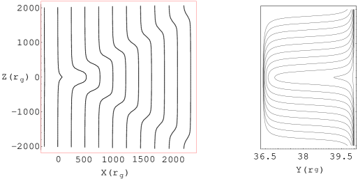
FIG. 5.: Reconstruction of perturbed string (Cartesian coordinates).

To summarize, the scattering of the string in the weak gravitational fields calculated in the first order in $\varphi$ results in the displacement of the string in the direction perpendicular to the motion by the value ${\chi}_{2}(\tau=\infty)=-2\pi GM\sinh\beta/c^{2}$. At any finite but large value of $\tau$ a solution represents a kink and anti-kink of the width $Y_{0}\coth\beta=Y_{0}c/v$ propagating in the opposite directions with the velocity of light and leaving behind them the string in the new “phase” with $Y=Y_{0}+{\chi}_{2}(\tau=\infty)$.

VI Low-Velocity Limit

As was already mentioned, the components $f_{R}$ normal to the string world-sheet are components of the physical force acting on the string. As can be seen from (36), the force $f_{R}$ acting on the string vanishes in the limit $v\rightarrow 0$. This fact has a simple physical explanation. As was shown in [5], a static string configuration in a static spacetime is a geodesic in a spacetime with the metric $|g_{00}|g_{ij}$, which in our case takes the form

$$dS^{2}=|g_{00}|g_{ij}dx^{i}dx^{j}=(1-2\Phi)(1+2\Psi)(dX^{2}+dY^{2}+dZ^{2})\,.$$ (65)

In the leading order, $\Phi=\Psi=\varphi$, and the string is a straight line [1]. In other words, in the first-order approximation a force acting on a static string in a static spacetime of a black hole vanishes. For this reason, the leading terms in the expansion of the force are of the second order in $\varphi$, and they remain so until $v/c\sim(GM/b_{imp})^{1/2}$. In this section we discuss the effect of these second order terms on the motion of the string in the limit of very small velocities.

Substituting (18) into the dynamical equations (3) we get

$$n^{\mu}_{R}\,\,\Box\stackrel{{\scriptstyle{2}}}{{\chi}}{}^{\!R}=\stackrel{{\scriptstyle{2}}}{{f}}{}^{\!\mu}\equiv A^{\mu}+B^{\mu}\,,$$ (66)

where the $\Box$-operator is given by (31) and,

$$A^{\mu}=-\eta^{AB}\stackrel{{\scriptstyle{2}}}{{\Gamma}}{}^{\!\mu}_{\alpha\beta}X^{\alpha}_{,A}X^{\beta}_{,B}\,,\hskip 14.22636ptB^{\mu}=-\eta^{AB}\stackrel{{\scriptstyle{1}}}{{\Gamma}}{}^{\!\mu}_{\alpha\beta}(\stackrel{{\scriptstyle{1}}}{{\chi}}{}^{\!m}_{,B}X^{\alpha}_{,A}e^{\beta}_{(m)}+\stackrel{{\scriptstyle{1}}}{{\chi}}{}^{\!m}_{,A}X^{\beta}_{,B}e^{\alpha}_{(m)})\,.$$ (67)

Note that

$$\stackrel{{\scriptstyle{2}}}{{\Gamma}}{}^{\!\mu}_{\alpha\beta}=\eta^{\mu\nu}\stackrel{{\scriptstyle{2}}}{{\Gamma}}_{\nu,\alpha\beta}+\stackrel{{\scriptstyle{1}}}{{\gamma}}{}^{\!\mu\nu}\stackrel{{\scriptstyle{1}}}{{\Gamma}}_{\nu,\alpha\beta}\,$$ (68)

where $\stackrel{{\scriptstyle{1}}}{{\Gamma}}_{\nu,\alpha\beta}$ is given by (30) and,

$$\stackrel{{\scriptstyle{2}}}{{\Gamma}}_{\nu,\alpha\beta}=2\varphi\,(\varphi_{,\alpha}\,\pi_{\nu\beta}+\varphi_{,\beta}\,\pi_{\nu\alpha}-\varphi_{,\nu}\,\pi_{\alpha\beta})\,.$$ (69)

We focus our attention on the corrections to the motion of the string in $Y$-direction. It is easy to verify that

$$A^{2}=\cosh^{2}\beta\stackrel{{\scriptstyle{2}}}{{\Gamma}}{}^{\!2}_{00}-\stackrel{{\scriptstyle{2}}}{{\Gamma}}{}^{\!2}_{33}=2\varphi\varphi_{,2}[(1-a)\cosh^{2}\beta-(1-b)]\,.$$ (70)

Calculations also give

$$B^{2}=2\varphi_{,2}\left[(\cosh^{2}\beta+\sinh^{2}\beta)\stackrel{{\scriptstyle{1}}}{{\chi}}_{0,0}-\sinh(2\beta)\stackrel{{\scriptstyle{1}}}{{\chi}}_{1,0}+\stackrel{{\scriptstyle{1}}}{{\chi}}_{3,3}\right]-2\varphi_{,3}\stackrel{{\scriptstyle{1}}}{{\chi}}_{2,3}\,.$$ (71)

At low velocities one has

$$A^{2}\sim 2\varphi\varphi_{,2}(b-a)\,,\hskip 14.22636ptB^{2}\sim 2\varphi_{,2}(\stackrel{{\scriptstyle{1}}}{{\chi}}_{0,0}+\stackrel{{\scriptstyle{1}}}{{\chi}}_{3,3})-2\varphi_{,3}\stackrel{{\scriptstyle{1}}}{{\chi}}_{2,3}\,.$$ (72)

Equation (46) shows that $\stackrel{{\scriptstyle{1}}}{{\chi}}_{2}$ vanishes at $\beta\rightarrow 0$. Using relation (27), we finally get

$$\stackrel{{\scriptstyle{2}}}{{f}}_{2}\sim-2(2+a-b)\varphi\varphi_{,2}\,.$$ (73)

Using a relation similar to (42) we get

$$\stackrel{{\scriptstyle{2}}}{{\chi}}_{2}(\tau=\infty)={2+a-b\over 2\sinh\beta}\,\int_{-\infty}^{\infty}{dX}\int_{-\infty}^{\infty}{dZ}\,\,{\partial\varphi^{2}\over\partial Y}(X,Y_{0},Z)\,.$$ (74)

Calculating the integral one gets

$$\stackrel{{\scriptstyle{2}}}{{\chi}}_{2}(\tau=\infty)=-{\pi M^{2}(2+a-b)\over Y_{0}\sinh\beta}\,.$$ (75)

For the scattering of the string on the Schwarzschild black hole, $a=-1$ and $b=3/4$, so that one has

$$\stackrel{{\scriptstyle{2}}}{{\chi}}_{2}(\tau=\infty)=-{\pi(GM)^{2}\over 4c^{4}Y_{0}\sinh\beta}\,.$$ (76)

Using the expressions for the coefficients $a$ and $b$ for the scattering on a Reissner-Nordstrom black hole (see footnote 1) one gets

$$\stackrel{{\scriptstyle{2}}}{{\chi}}_{2}(\tau=\infty)=-{\pi((GM)^{2}-GQ^{2})\over 4c^{4}Y_{0}\sinh\beta}\,.$$ (77)

These results are in the complete agreement with the results obtained by Page [10].

VII Conclusions

We analyzed the motion of a cosmic string in the gravitational field of a black hole in the approximation where the field is weak. In particular, we demonstrated that after passing the black hole, the string continues its motion with the same velocity $\bf v$ as before scattering, but it is displaced in the direction to the black hole and perpendicular to $\bf v$ by the distance $\Delta b\sim-2\pi GM\sinh\beta/c^{2}-\pi(GM)^{2}/(4c^{3}vb_{imp})$, where $b_{imp}$ is the impact parameter. If $|b_{imp}-\Delta b|\gg r_{g}=2GM/c^{2}$ the string moves always in a weak field. If $|b_{imp}-\Delta b|\sim r_{g}=2GM/c^{2}$ the string enters the strong-field region near the black hole and it can be captured. This allows us to give the following estimate of the critical capture impact parameter. For low velocity, $(v/c)\ll 1$,

$$b_{capture}\sim{GM\over c^{2}}\left(\pi\over 4\right)^{1/2}\,\left(v\over c\right)^{-1/2}\,.$$ (78)

For $v/c>(GM/b_{imp})^{1/2}$ the first term in $\Delta b$ dominates. This means that the capture impact parameter grows for both small and large values of $v/c$, and hence there exists a velocity $v$ for which the capture impact parameter has minimum value. This conclusion is confirmed by the results of the numerical computations of the capture impact parameter [9]. The numerical results demonstrate also that for the ultrarelativistic velocities the critical impact parameter $b_{capture}$ reaches the value $3\sqrt{3}GM/c^{2}$, that is the same value as the capture parameter for the ultrarelativistic particles.

Besides giving us a qualitative understanding of the scattering and capture of cosmic strings by black holes, the analysis of the weak-field approximation is important for the numerical study of these processes in the strong field. Before and after the scattering the string moves far from the black hole, where the gravitational field is weak. Thus one can use the above analysis to provide a well-defined description of “in”- and “out”-states of the string and to formulate the scattering problem. We discuss this in Ref.[9].

Acknowledgments:  This work was partly supported by the Natural Sciences and Engineering Research Council of Canada. One of the authors (V.F.) is grateful to the Killam Trust for its financial support. The authors are grateful to Arne Larsen for early insights into the perturbative equations of motion. The authors are also grateful to Don Page, who made his paper [10] available prior to publication. We also thank him for various discussions.

REFERENCES

• [1] E. P. S. Shellard and A. Vilenkin, Cosmic Strings. (Cambridge Univ. Press, Cambridge) (1994).
• [2] V.P. Frolov, S. Hendy, and A.L. Larsen, Phys. Rev. D54, 5093 (1996).
• [3] V.P. Frolov, S. Hendy, and J.P. De Villiers, Class.Quant.Grav. 14, 1099 (1997).
• [4] A.M. Polyakov, Phys. Lett. B103, 207-210 (1981).
• [5] V.P. Frolov, V.D. Skarzhinsky, A.I. Zelnikov, and O. Heinrich, Phys. Lett. B224, 255 (1989).
• [6] B. Carter and V.P. Frolov, Class.Quant.Grav. 6 569 (1989).
• [7] S. Lonsdale and I. Moss, Nucl. Phys. B298, 693 (1988).
• [8] J.P. De Villiers and V.P. Frolov, Gravitational Capture of Cosmic Strings by a Black Hole. Preprint, Alberta Thy 14-97; gr-qc/9711045.
• [9] J.P. De Villiers and V.P. Frolov, Gravitational Scattering of Cosmic Strings by a Black Hole. (paper under preparation).
• [10] D.N. Page Gravitational Capture and Scattering of Straight Test Strings with Large Impact Parameters Preprint, Alberta Thy 05-98; gr-qc/98mmddnn.
• [11] C.W. Misner, K.S. Thorne, and J.A. Wheeler, Gravitation (W.H. Freeman, San Francisco, 1973).
• [12] G.W. Gibbons and M.J. Perry, Nucl. Phys. B146, 90 (1978).
• [13] V.P. Frolov and A.L. Larsen, Nucl. Phys. B414, 129 (1988).