COSMIC GRAVITATIONAL WAVE BACKGROUND
IN STRING COSMOLOGY

String cosmology models predict a stochastic cosmic background of gravitational waves with a characteristic spectrum. I describe the background, present astrophysical and cosmological bounds on it, and outline how it may be possible to detect it with gravitational wave detectors.

1 Introduction

A robust prediction of models of string cosmology which realize the pre-big-bang scenario $\!{}^{{\bf?},{\bf?}}$ is that our present-day universe contains a cosmic gravitational wave background $\!{}^{{\bf?},{\bf?},{\bf?}}$, with a spectrum which is quite different than that predicted by many other early-universe cosmological models $\!{}^{{\bf?},{\bf?},{\bf?},{\bf?}}$. In the pre-big-bang scenario the evolution of the universe starts from a state of very small curvature and coupling and then undergoes a long phase of dilaton-driven kinetic inflation reaching roughly Planckian energy densities $\!{}^{{\bf?}}$, and at some later time joins smoothly standard radiation dominated cosmological evolution, thus giving rise to a singularity free inflationary cosmology.

It is the purpose of this talk to explain the properties of the cosmic gravitational wave background predicted by string cosmology, to explain astrophysical and cosmological bounds on its shape and strength and to show that currently operating and planned gravitational wave detectors could further constrain the spectrum and perhaps even detect it. The emphasis is on the general properties of the spectrum and the basic experimental setup needed for its detection, rather than on precise numerical estimates and technical details.

Because the gravitational interaction is so weak, a background of gravitational radiation decouples from the matter in the universe at very early times and carries with it a picture of the state of the universe when energy densities and temperatures were extreme. The weakness of the gravitational interaction makes a detection of such a background very hard, and necessitates a strong signal. String cosmology provides perhaps the strongest source possible: the whole universe, accelerated to roughly Planckian energy densities. A discovery of any primordial gravitational wave background, and in particular, the one predicted by string cosmology, could therefore provide unrivaled exciting information on the very early universe.

2 Cosmic gravitational wave background in string cosmology

In models of string cosmology $\!{}^{{\bf?}}$, the universe passes through two early inflationary stages. The first of these is called the “dilaton-driven” period and the second is the “string” phase. Each of these stages produces stochastic gravitational radiation by the standard mechanism of amplification of quantum fluctuations $\!{}^{{\bf?}}$. Deviations from homogeneity and isotropy of the metric field are generated by quantum fluctuations around the homogeneous and isotropic background, and then amplified by the accelerated expansion of the universe. The transverse and traceless part of these fluctuations are the gravitons. In practice, we compute graviton production by solving linearized perturbation equations with vacuum fluctuations boundary conditions. The production strength of gravitons depends on the curvature and coupling. Since at the end of the accelerated expansion phase curvatures reach the string curvature, and the coupling reaches approximately today’s coupling, graviton production is expected to be at the strongest possible level.

In order to describe the background of gravitational radiation, it is conventional to use a spectral function $\Omega_{\rm GW}(f)={1\over\rho_{\rm critical}}{d\rho_{\rm GW}\over d\ln f}.$ Here $d\rho_{\rm GW}$ is the (present-day) energy density in stochastic gravitational waves in the frequency range $d\ln f$, and $\rho_{\rm critical}$ is the critical energy-density required to just close the universe, $\rho_{\rm critical}={3c^{2}H_{0}^{2}\over 8\pi G}\approx 1.6\times 10^{-8}{\rm h}_{100}^{2}\rm\>ergs/cm^{3},$ where the Hubble expansion rate $H_{0}$ is the rate at which our universe is currently expanding, $H_{0}={\rm h}_{100}\>100\>{\rm Km\over sec-Mpc}=3.2\times 10^{-18}{\rm h}_{100}{\rm 1\over sec}.$ ${\rm h}_{100}$ is believed to lie in the range $0.5<{\rm h}_{100}<0.8$. The spectral function is related to the dimensionless strain $h$, $\Omega_{\rm GW}(f)\simeq 10^{36}h_{100}^{-2}(f/{\rm Hz})^{2}h(f)^{2}$ and to the strain in units $1/\sqrt{Hz}$, $\sqrt{S_{h}(f)}$, $\Omega_{\rm GW}(f)\simeq 10^{36}h_{100}^{-2}(f/{\rm Hz})^{3}S_{h}(f)$.

The spectrum of gravitational radiation produced in the dilaton-driven (and string) phase was estimated in [3], $\Omega_{GW}(f)\simeq z_{eq}^{-1}g_{s}^{2}\left(f\over f_{S}\right)^{3}\left[1+z_{S}^{-3}\left(g_{1}\over g_{S}\right)^{2}\right],f<f_{S},$ where some logarithmic correction factors were dropped. The coupling $g_{1}$ is today’s coupling, assumed to be constant from the end of the string phase until today, $g_{S}$ is the coupling at the end of the dilaton-driven phase, and $f_{S}$ is the frequency marking the end of the dilaton-driven phase. The frequency $f_{1}=f_{S}z_{S}$ is the frequency at the end of the string phase, where $z_{S}$ is the total redshift during the string phase and $z_{eq}\sim 10^{4}$ is the redshift from matter-radiation equality until today. The spectrum can be expressed in a more symmetric form $\!{}^{{\bf?}}$, $\Omega_{GW}(f)\simeq z_{eq}^{-1}g_{1}^{2}\left(\frac{f}{f_{1}}\right)^{3}\left[z_{S}^{3}(g_{S}/g_{1})^{2}+z_{S}^{-3}(g_{S}/g_{1})^{-2}\right].$ Note that the spectrum is invariant under the exchange $z_{s}^{3}(g_{s}/g_{1})^{2}\leftrightarrow z_{s}^{-3}(g_{s}/g_{1})^{-2}$ and that this implies a lower bound on the spectrum, $\Omega_{GW}(f)\raise 1.72218pt\hbox{$>$}\kern-6.99997pt\lower 2.6694pt\hbox{$\sim$}2z_{eq}^{-1}g_{1}^{2}\left(\frac{f}{f_{1}}\right)^{3}.$ The lower bound is obtained for the “minimal spectrum” with $z_{S}=1$ and $g_{S}/g_{1}=1$ describing a cosmology with almost no intermediate string phase.

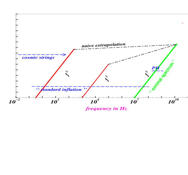
Figure 1: Spectrum of GW background. The minimal spectrum discussed in the text and two other possible spectra are shown. Also shown are estimated spectra in other cosmological models.

In the simplest model, which we will use to estimate the spectrum and prospects for its detection, the spectrum depends upon four parameters. The first pair of parameters are the maximal frequency $f_{1}$ above which gravitational radiation is not produced and $g_{1}$, the coupling at the end of the string phase. The second pair of these are $z_{S}$ and $g_{S}$. The second pair of parameters can be traded for the frequency ${f_{\rm S}}=f_{1}/z_{S}$ and the fractional energy density $\Omega^{\rm S}_{\rm GW}=\Omega_{\rm GW}(f_{S})$ produced at the end of the dilaton-driven phase. At the moment, we cannot compute $g_{S}$ and $z_{S}$ from first principles, because they involve knowledge of the evolution during the high curvature string phase. We do, however, expect $z_{S}$ to be quite large. Recall that $z_{S}$ is the total redshift during the string phase, and that during this phase the curvature and expansion rate are approximately string scale, therefore, $z_{S}$ grows roughly exponentially with the duration (in string times) of this phase. Some particular exit models $\!{}^{{\bf?}}$ suggest that $z_{S}$ could indeed be quite large. I cannot estimate, at the moment, a likely range for the ratio $g_{1}/g_{S}$ except for the reasonable assumption $g_{1}/g_{S}>1$.

A useful approximate form for the spectrum in the range $z_{S}>1$ and $g_{1}/g_{S}\raise 1.72218pt\hbox{$>$}\kern-6.99997pt\lower 2.6694pt\hbox{$\sim$}1$ is the following $\!{}^{{\bf?}}$

$$\Omega_{\rm GW}(f)=\cases{{\Omega^{\rm S}_{\rm GW}(f/{f_{\rm S}})^{3}}&{ $f<{f_{\rm S}}$}\cr&\cr{\Omega^{\rm S}_{\rm GW}(f/{f_{\rm S}})^{\beta}}&${f_{\rm S}}<f<f_{1}$\cr&\cr{0}&$f_{1}<f$}$$ (1)

where $\beta=\frac{\log\left[\Omega_{\rm GW}(f_{1})/\Omega^{\rm S}_{\rm GW}\right]}{\log\left[f_{1}/{f_{\rm S}}\right]}$ is the logarithmic slope of the spectrum produced in the string phase (see also other models $\!{}^{{\bf?}}$). If we assume that there is no late entropy production and make reasonable choices for the number of effective degrees of freedom, then two of the four parameters may be determined in terms of the Hubble parameter $H_{\rm r}$ at the onset of radiation domination immediately following the string phase of expansion $\!{}^{{\bf?}}$, $f_{1}=1.3\times 10^{10}\>{\rm Hz}\left({H_{\rm r}\over 5\times 10^{17}\>{\rm GeV}}\right)^{1/2}$ and $\Omega_{\rm GW}(f_{1})=1\times 10^{-7}{\rm h}_{100}^{-2}\left({H_{\rm r}\over 5\times 10^{17}\>{\rm GeV}}\right)^{2}.$ Spectra for some arbitrarily chosen parameters and possible backgrounds from other cosmological models are shown in Fig. 1. The label PH denotes preheating after inflation $\!{}^{{\bf?}}$.

3 Astrophysical and cosmological bounds

At the moment, the most restrictive observational constraint on the spectral parameters comes from the standard model of big-bang nucleosynthesis (NS) $\!{}^{{\bf?}}$. This restricts the total energy density in gravitons to less than that of approximately one massless degree of freedom in thermal equilibrium. This bound implies that $\!{}^{{\bf?}}$

$$\int\Omega_{\rm GW}(f)d\ln f=\Omega_{\rm GW}^{\rm S}\left[\frac{1}{3}+\frac{1}{\beta}\left(\left(f_{1}/f_{\rm S}\right)^{\beta}-1\right)\right]<0.7\times 10^{-5}{\rm h}^{-2}_{100}.$$ (2)

where we have assumed an allowed $N_{\nu}=4$ at NS, and have substituted in the spectrum (1). The NS bound and additional cosmological and astrophysical bounds are shown in Fig. 2, where $h_{100}$ was set to unity.

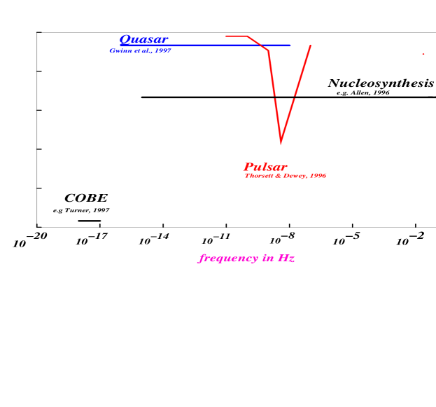
Figure 2: Cosmological and astrophysical upper bounds on the cosmic gravitational wave background.

The line marked “Quasar” in Fig. 2 corresponds to a bound coming from quasar proper motions. A stochastic background of gravity waves (GW) makes the signal from distant quasars scatter randomly on its way to earth. This may cause quasar proper motions. An upper bound on quasar proper motions can be translated into an upper bound on a stochastic background $\!{}^{{\bf?}}$. A typical strain $h$ may induce proper motion $\mu$, $h/f\sim\mu$. The sensitivity reached was approximately microarcsecond per year $\!{}^{{\bf?}}$, corresponding to a dimensionless strain of about $h\sim 5\times 10^{-9}$ at frequencies below the observation time: approximately (20 years)${}^{-1}\sim 5\times 10^{-9}Hz$, leading to $\Omega_{GW}\raise 1.72218pt\hbox{$<$}\kern-8.00003pt\lower 2.6694pt\hbox{$\sim$}0.1h_{100}^{-2}$.

The line marked “COBE” in Fig. 2 corresponds to the bound coming from energy density fluctuations in the cosmic microwave background, which can be expressed in terms of the measured temperature fluctuations $\Delta T/T$, $\Omega({\rm perturbations})\simeq(\frac{\Delta T}{T})^{2}\Omega_{\gamma}\sim 10^{-10}\times 10^{-4}=10^{-14}h_{100}^{-2}$. Since it is known $\!{}^{{\bf?}}$ that $\Omega_{GW}\raise 1.72218pt\hbox{$<$}\kern-8.00003pt\lower 2.6694pt\hbox{$\sim$}0.1\Omega({\rm perturbations})$, it follows that $\Omega_{GW}h_{100}^{2}\raise 1.72218pt\hbox{$<$}\kern-8.00003pt\lower 2.6694pt\hbox{$\sim$}10^{-15}$ at frequencies $10^{-18}h_{100}Hz-10^{-16}h_{100}Hz$.

The curve marked “Pulsar” represents the bound coming from millisecond pulsar timing $\!{}^{{\bf?}}$. Assuming known distance and signal emission times, the pulsar functions as a giant one-arm interferometer. The statistics of pulse arrival time residuals $\Delta T$, puts an upper bound on any kind of noise in the system, including a stochastic background of GW. The typical strain sensitivity is $h\sim\frac{\Delta T}{T}$, where $T$ is the total observation time, reaching by now 20 years $\sim 6\times 10^{8}sec$ and $\Delta T\sim 10\mu s$ is the accuracy in measuring time residuals. Translated into $\Omega_{GW}(f)$, this yields the bound shown in the figure, which is most restrictive at frequencies $f\sim 1/T\sim 5\times 10^{-9}Hz$.

Notice that all the existing bounds are in the very low frequency range, while the expected signal from string cosmology is in a higher frequency range. The bounds are therefore not very restrictive.

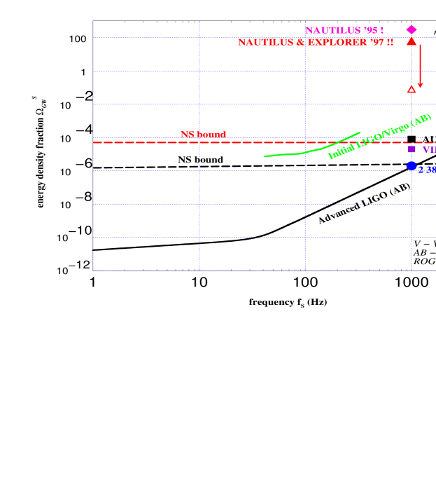
Figure 3: Detection sensitivity of relic GW by operating and planned GW detectors. The interesting region of parameter space is below the “NS bound” lines.

4 Detecting a string cosmology stochastic gravitational wave background

A number of authors $\!{}^{{\bf?},{\bf?},{\bf?}}$ have shown how one can use a network of two or more gravitational wave antennae to detect a stochastic background of gravitational radiation. The basic idea is to correlate the signals from separated detectors, and to search for a correlated strain produced by the gravitational wave background, which is buried in the instrumental noise. It has been shown by these authors that after correlating signals for time $T$ the ratio of “Signal” to “Noise” (squared) is given by an integral over frequency $f$:

$$\left({S\over N}\right)^{2}={9H_{0}^{4}\over 50\pi^{4}}T\int_{0}^{\infty}df\>{\gamma^{2}(f)\Omega_{\rm GW}^{2}(f)\over f^{6}P_{1}(f)P_{2}(f)}.$$ (3)

The instrument noise in the detectors is described by the one-sided noise power spectral densities $P_{i}(f)$. The LIGO project is building two identical detectors, which we will refer to as the “initial” detectors. These detectors will be upgraded to so-called “advanced” detectors. Since the two detectors are identical in design, $P_{1}(f)=P_{2}(f)$. The design goals for the detectors specify these functions $\!{}^{{\bf?}}$. The design noise power spectrum for the Virgo detector $\!{}^{{\bf?}}$ and noise power spectral densities of operating and planned resonant mass GW detectors (“bars”) $\!{}^{{\bf?},{\bf?}}$ are also known. The overlap reduction function $\gamma(f)$ is determined by the relative locations and orientations of the two detectors. It is identical for both the initial and advanced LIGO detectors, and has been determined for many pairs of GW detectors $\!{}^{{\bf?},{\bf?}}$.

Making use of the prediction from string cosmology (1), we may use equation (3) to assess the detectability of this stochastic background. For any given set of parameters we may numerically evaluate the signal to noise ratio $S/N$; if this value is greater than $1.65$ then with at least 90% confidence, the background can be detected by a given pair of detectors. The regions of detectability in parameter space are shown in Fig. 3. The region below the NS bound lines and above the advanced LIGO curve is the region of interest. Two NS bounds are shown, the upper, more relaxed bound, assumes no GW production during the string phase $\!{}^{{\bf?}}$. The points at 1 KHz come from operating and planned resonant mass detectors. Some are taken from real experiments, an upper bound from a single detector run $\!{}^{{\bf?}}$, and the first modern 12.5 hours correlation experiment between Nautilus and Explorer $\!{}^{{\bf?}}$. The arrow points to a hollow triangle showing by how much the correlation experiment can be improved if Nautilus works properly and the experiment could be done for one year. Other points are from theoretical calculations $\!{}^{{\bf?}}$. For Fig. 3 we have assumed ${\rm h}_{100}=0.65$ and $H_{\rm r}=5\times 10^{17}\>{\rm GeV}$.

References

References

- [1] G. Veneziano, Phys. Lett. B265 (1991) 287.
- [2] M. Gasperini and G. Veneziano, Astropart. Phys. 1 (1993) 317.
- [3] R. Brustein, M. Gasperini, M. Giovannini and G. Veneziano Phys. Lett. B361 (1995) 45.
- [4] M. Gasperini and M. Giovannini, Phys. Rev. D47 (1993) 1519.
- [5] M. Gasperini, in proceedings of the 2nd Edoardo Amaldi Conference on Gravitational Waves, Geneva, Switzerland, 1-4 Jul 1997, gr-qc/9707034.
- [6] L.P. Grishchuk, Sov. Phys. JETP 40 (1975) 409.
- [7] M. S. Turner, Phys. Rev. D55 (1997) 435.
- [8] B. Allen, in Proceedings of the Les Houches School on Astrophysical Sources of Gravitational Radiation, Springer-Verlag, 1996.
- [9] M. Maggiore, gr-qc/9803028.
- [10] R. Brustein and G. Veneziano, Phys. Lett. B329 (1994) 429; N. Kaloper, R. Madden and K.A. Olive, Nucl. Phys. B452 (1995) 677.
- [11] N.D. Birrell and P.C.W. Davies, Quantum fields in curved space, Cambridge University Press 1984; V. F. Mukhanov, A. H. Feldman and R. H. Brandenberger, Phys. Rep. 215 (1992) 203.
- [12] R. Brustein, M. Gasperini and G. Veneziano, hep-th/9803018.
- [13] M. Gasperini, M. Maggiore and G. Veneziano, Nucl. Phys. B494 (1997) 315; R. Brustein and R. Madden, Phys. Lett. B410 (1997) 110; R. Brustein and R. Madden Phys. Rev. D57 (1998) 712.
- [14] R. Brustein, in Cascina 1996, Gravitational waves pp. 149-152, hep-th/9604159.
- [15] A. Buonanno, M. Maggiore and C. Ungarelli , Phys. Rev. D55 (1997) 3330; M. Galluccio, M. Litterio and F. Occhionero, Phys. Rev. Lett. 79 (1997) 970; M. Maggiore, Phys. Rev. D56 (1997) 1320; M. Gasperini, Phys. Rev. D56 (1997) 4815.
- [16] R. Brustein, M. Gasperini and G. Veneziano, Phys. Rev. D55 (1997) 3882.
- [17] S. Y. Khlebnikov and I. I. Tkachev, Phys. Rev. D56 (1997) 653.
- [18] V. F. Schwartzmann, JETP Lett. 9 (1969) 184; T. Walker et al., Ap. J. 376 (1991) 51.
- [19] B. Allen and R. Brustein, Phys. Rev. D55 (1997) 3260;
- [20] Carl R. Gwinn et al., Ap. J. 485 (1997) 87.
- [21] S. E. Thorsett and R. J. Dewey, Phys. Rev. D53 (1996) 3468.
- [22] P. Michelson, MNRAS 227 (1987) 933; N. Christensen, Phys. Rev. D46 (1992) 5250; E. Flanagan, Phys. Rev. D48 (1993) 2389.
- [23] S. Vitale, M. Cerdonio, E. Coccia and A. Ortolan, Phys. Rev. D55 (1997) 1741.
- [24] B. Allen and J. D. Romano, gr-qc/9710117.
- [25] A. Abramovici, et. al., Science 256 (1992) 325.
- [26] B. Caron et al., Class. Quant. Grav. 14 (1997) 1461.
- [27] P. Astone et al., ROG collaboration, Astropart. Phys. 7 (1997) 231.
- [28] M. Cerdonio et al., Class. Quant. Grav. 14 (1997) 1491.
- [29] P. Astone et al., ROG collaboration, Phys. Lett. B385 (1997) 421.
- [30] P. Astone, et al., ROG collaboration, to appear in Proceedings of the Eighth Marcel Grossmann Meeting, (World Scientific, 1998).