Event Horizons in Numerical Relativity II: Analyzing the Horizon

Abstract

We present techniques and methods for analyzing the dynamics of event horizons in numerically constructed spacetimes. There are three classes of analytical tools we have investigated. The first class consists of proper geometrical measures of the horizon which allow us comparison with perturbation theory and powerful global theorems. The second class involves the location and study of horizon generators. The third class includes the induced horizon 2-metric in the generator comoving coordinates and a set of membrane-paradigm like quantities. Applications to several distorted, rotating, and colliding black hole spacetimes are provided as examples of these techniques.

I Introduction

Black holes play an important role in general relativity and astrophysics. They are characterized both by spacetime singularities within them and by their horizons that cover the singularities from the outside world. In this paper we develop a set of tools for analyzing the dynamics of black hole horizons.

The event horizon (EH) of a black hole is defined as the boundary of the causal past of future null infinity $\mathcal{I}^{+}$. As such the EH surface is traced out by light rays that never reach future null infinity and never fall into the black hole singularity. This surface responds to infalling matter and radiation and to the gravitational fields of external bodies. In the membrane paradigm of black holes, the horizon fully characterizes the dynamical interactions of a black hole with its surroundings [1]. The important role of the horizon in the study of black holes motivates us to carry out a systematic study of horizon dynamics in numerical relativity.

While much work has been done on the properties of stationary black holes and small perturbations about them, little is known about the properties of highly dynamical black hole spacetimes. For example, the cosmic censorship conjecture [2], which suggests that spacetime singularities should be clothed by event horizons, demands study into the existence of horizons. The hoop conjecture [3, 4], which states that a black hole horizon forms if and only if a matter source becomes sufficiently compact in all directions, begs the question of how spherical must a black hole horizon be. Caustics, or singular points in the congruence of photons tracing out the horizon where new generators can join the horizon, can occur, but under what conditions do they appear? And what are the properties of these caustics? One would also like to know to what extent one can understand interactions of black holes with their astrophysical environment in terms of properties of the EH. Studies of most of these questions have to date only been made in very idealized circumstances or quasi-stationary spacetimes. But aspects of each of these open questions are amenable to study with the numerical methods we describe.

Due to strong field nonlinearities, black hole horizons are difficult to study analytically. Therefore we turn to numerical treatment which is now routinely able to generate highly dynamical, axisymmetric black hole spacetimes evolved beyond $t=100M$, where $M$ is the ADM mass of the spacetime. Many such axisymmetric studies of highly distorted rotating and non-rotating black holes and colliding black holes have been performed in recent years[5, 6, 7, 8]. Three dimensional black hole evolutions are approaching the accuracy of axisymmetric calculations[9, 10, 11, 12, 13]. Together with the ability to find and analyze event horizons, these simulations provide us with a new opportunity to study black hole dynamics.

We recently proposed methods for the study of the EH in numerically generated spacetimes [14]. In a series of followup papers, we give details of the methods and their applications to various black hole spacetimes. The first paper in this series[15], referred to hereafter as Paper I, detailed the method for locating the EH in a dynamical spacetime, and showed the high degree of accuracy with which the EH can be located. In this second paper, we focus on the tools constructed for analyzing the dynamics of the EH.

There are several aims of the present paper. We show three different sets of tools that can be used to analyzing the dynamics of the EH, and how one can construct them in numerical relativity. We show how accurately the quantities used in these tools can be constructed with present numerically generated black hole spacetimes. We demonstrate the applicability of these tools to various spacetimes of interest. In fact, these tools apply immediately to almost all numerically generated black hole spacetimes we have constructed to date. This paper describes the tools that elucidate the physics of the EH, and the accuracy with which we can (or cannot) evaluate these measures; the emphasis is not on the physics itself. The physics we learn using these tools will be discussed in a later paper in this series.

We have developed and present three sets of tools for analyzing the EH. First, we present a set of geometric measures of the horizon as a two dimensional surface in a curved 3D space-like slice of constant time. These tools include proper circumferences, proper area, Gaussian curvature, the embedding of the surface in Euclidean space, and the embedding history. Second, we discuss how the horizon generators can be constructed. This construction also gives the locus of generators that will join the horizon in the future at caustic points on the horizon surface. Third, we present a set of tools from the membrane paradigm of black holes[1] for analyzing the generators and the physics they contain, such as the horizon 2–metric in generator co-moving coordinates, $\gamma^{H}_{ab}$ and quantities derived from and connected to it, such as the expansion $\Theta^{H}$, shear $\sigma^{H}_{ab}$, surface gravity $g_{H}$, and Hajicek field $\Omega^{H}_{a}$.

To illustrate the use of these horizon tools, we apply them to several spacetimes. We consider the Schwarzschild and Kerr analytic black hole spacetimes to show the basic principles involved, and to test the accuracy of the methods. Also, we apply them to fully nonlinear, highly dynamical black hole systems, such as a distorted Schwarzschild BH, a distorted Kerr BH, and the collision of two black holes (the Misner data[16]). Our tools can be applied to almost all numerical black hole spacetimes we have presently constructed, and should be applicable to future black hole spacetimes as well.

The structure of this paper is as follows: In Sec. II we briefly review the method we developed to find the location of the EH. In Sec. III we show various ways to extract important information from the EH surface location in the spacetime, including studying the topology, area, various circumferences, Gaussian curvature, and geometric embeddings of the surface. In Sec. IV we show how to find the actual generators of the EH, and the information their paths can bring. In Sec. V we discuss how one can apply ideas developed in the membrane paradigm[1] to numerically generated black hole spacetimes. Throughout the paper, we illustrate these ideas with examples from numerically generated black hole spacetimes.

II Locating the EH in a Numerically Generated Black Hole Spacetime

Our method for locating event horizons in numerical relativity was detailed in Paper I. In order to define our notation, and because our analysis here is closely related to our EH finding method, we briefly review it here. The essence of the EH finding method can be summarized in four steps:

(i) At late times after the dynamical evolution we seek to analyze (that is, when the black hole spacetime has returned to approximate stationarity; e.g., after the coalescence of two black holes or after all incident gravitation radiation has either radiated into the hole or into the far wave zone) the position of the EH can often be located approximately. We can identify a region of the late-time spacetime which contains the EH, which we call the horizon containing domain (HCD).

(ii) We trace the evolution of the HCD backward in time by tracing its outer and inner boundaries as null surfaces. A function describing a null surface at $t=t_{f}$, $x^{i}=x_{f}^{i}$

$$f(t=t_{f},x^{i}_{f})=0,$$ (1)

satisfies the equation

$$\partial_{\mu}f\partial^{\mu}f=0,$$ (2)

or,

$$\partial_{t}f=\frac{-g^{ti}\partial_{i}f+\sqrt{(g^{ti}\partial_{i}f)^{2}-g^{tt}g^{ij}\partial_{i}f\partial_{j}f}}{g^{tt}}.$$ (3)

for outgoing surfaces. The fact that this method represents the position of the EH directly as a function $f(t,x^{i})$ is particularly convenient in our construction of horizon analysis tools, as we shall see below.

(iii)The strength of our method stems from the fact that the inner and outer boundaries of the HCD converge together quickly when integrated backwards in time in many cases of interest. When the distance between the two boundaries in a time slice becomes significantly less than the grid separation used in the construction of the spacetime, we have accurately located the EH. This condition can often be met through the entire regime of interest here.

(iv) The choice of parameterization of the surface is important. For the axisymmetric spacetimes used as examples in this paper, one convenient choice is

$$f=\eta-s(t,\theta)$$ (4)

where $\eta$ is a radial coordinate and $\theta$ is polar angular coordinate. In what follows, we assume that this function $f(t,\eta,\theta)$ has been obtained for the numerically constructed spacetime.

In axisymmetric two black hole spacetimes, such as those generated in [7, 17, 18], we can use the parameterization in Eq. (4) to trace the event horizon through the merger phase. In the Čadež coordinate system [19] where coordinates are centered around each individual throat and the axis below the throat is a line of constant $\theta$, this parameterization allows us to trace a single hole by applying an upwinded condition on the horizon at the axis before coalescence. In the recently proposed “Class I” coordinate system [18] where the coordinates are centered around the throat and the axis, forming peanut shaped radial coordinate lines near the throats, this parameterization will represent a null surface which contains both the horizon and the null surface which represents the locus of generators waiting to join the horizon; a simple symmetry boundary condition on the equator suffices. The locus can also be located in the Čadež system by using an alternate $(\rho,z)$ parameterization, as described in Paper I. We will use simulations generated in both coordinate systems interchangeably here.

III Studying the EH Surface

A Topology of the EH

We note that one important, but easy to obtain piece of information contained in $f(t,x^{i})=0$ is the topology of the EH at a constant time slice. In this section we show an interesting case of the EH undergoing a change of topology. We apply our EH finding method above to a numerically generated spacetime representing the head–on collision of two equal mass black holes with axisymmetry. In Fig. 1 we show the function $f(t,x^{i})=0$ at two times for the case of Misner time symmetric initial data, described by two throats connecting two identical asymptotically flat sheets, evolved by a code described in Ref. [7] (the “Čadež” code). The case considered here is for the Misner parameter $\mu=2.2$, for which the initial distance between the throats is $8.92M$, where $M$ is the $1/2$ the ADM mass. For details of the initial data set, see Ref. [16, 7].

FIG. 1.: We show the topology of the EH for the collision of two black holes using data generated with the Čadež code from the Misner $\mu=2.2$ initial data. The solid lines show the EH at $t=0M$ and $t=7.5M$. The dotted line at $t=0M$ shows the locus of generators which will join the horizon in the future. We note that between $t=0M$ and $t=7.5M$ the horizon undergoes a non-trivial topology change. We note that “crossover” type caustics form on the axis. We shall see below that new generators join the horizon at these points.

At $t=0$ the EH has the topology of two disconnected two spheres represented by the solid lines centered near $z=\pm 1$ in the $\rho-z$ plane. We note that the function $f(t=0,x^{i})$ gives not just the location of the EH, but also the locus of the future horizon generators before they join the horizon. At $t=7.5M$ the horizon has the topology of a single sphere.

We treat this change of EH topology by following the surface function backwards in time. We can trace the horizon from $t=75$ or $100M$ to a “dumbell” shaped horizon at $t=7.5M$. In Fig. 1, we start with this “dumbell” shaped horizon. Tracing this surface backward towards $t=0M$, we see that the central part of the surface shrinks rapidly, and the left and right hand sides cross, indicating the change in topology. At $t=0$ the portion of the surface corresponding to the locus of photons which will join the horizon, but have not yet done so, is given as a dashed line. As discussed in Sec.IV, the crossing of the surface signals that photons are leaving the horizon, going backwards in time. The crossed portion of the surface (shown as a dashed line in Fig.1) is no longer on the EH, but represents the surface of horizon generators “waiting to be born”, as they will join the horizon at a future time. For the work here, we define a point on the horizon where generators cross as a caustic, and therefore, at the point where the generators cross and join the horizon, the horizon has a caustic point. This caustic at the cusp in the event horizon is discussed further below, and also in Ref. [20].

B Geometry of the EH Surface

The function for the surface $f(t,x^{i})$, together with the metric induced on the surface, gives the intrinsic geometry of the EH, from which important physical properties can be determined. In this section we present a set of tools which allow one to study the intrinsic properties of the surface.

1 Area

There has been extensive study of the surface area of black hole event horizons in general relativity [21]. The area plays a central role in the thermodynamics of black holes. As area is a quantity directly used in analytic studies, it is important to be able to study the dynamical evolution of the area of the EH in a numerically constructed spacetime, both for understanding the spacetime, and also as a diagnostic tool for the accuracy of the numerical treatment.

Construction of the surface area as function of time is straightforward. Here we show how one computes the area mainly for establishing the notation used in this paper. A surface $f(t_{0},x^{i})=0$ determines the coordinate location $x^{i}=x^{i}(\bar{\theta},\bar{\phi}),(i=1,2,3)$, of the surface at time $t_{0}$, where we regard the surface as being parametrized by two surface coordinates $\bar{x}^{a}=(\bar{\theta},\bar{\phi}),(a=1,2)$. Denote the spatial line element of the spacelike hypersurface at $t=t_{0}$ by

$$d\sigma^{2}=g_{ij}\,dx^{i}\,dx^{j},$$ (5)

and so we can define an induced horizon 2–metric as

$$\gamma_{ab}=g_{ij}\frac{\partial x^{i}}{\partial\bar{x}^{a}}\frac{\partial x^{j}}{\partial\bar{x}^{b}}.$$ (6)

The surface area at a time $t$ is then given by

$$A(t)=\int{}\sqrt{\gamma}\,d\bar{x}^{1}\,d\bar{x}^{2},$$ (7)

where $\gamma$ is the determinant of $\gamma_{ab}$.

In Fig. 2 we show $A(t)$ for a Schwarzschild black hole evolved with maximal slicing. The dotted line (labeled Standard ADM) shows the results obtained using the standard numerical treatment as described in Ref.[22]. In this case, the calculation is carried out using a 1D code with 200 grid zones. It is well known that when evolved with such slicings and without shift, the EH will expand outward in the radial direction in coordinate space. At the same time, a sharp peak in the radial metric function develops near the EH. Due to numerical error caused by the inability to resolve this sharp peak, the function $A(t)$ deviates significantly from the analytic value of $16\pi M^{2}$ as the evolution continues.

FIG. 2.: We show the area of the EH traced out for a Schwarzschild spacetime evolved with two different methods. The dotted line shows the EH evolution with a standard 3+1 ADM evolution scheme. The dashed line shows the evolution with an apparent horizon boundary condition. The solid line shows the analytic value. We note that the same method is used for both spacetimes. The error in the standard ADM spacetime is due to inaccuracies in the spacetime metric, not the EH finder.

We compare this result to the case of the dashed line in Fig. 2, which is obtained by applying Eq. (7) to a Schwarzschild spacetime constructed with the same grid parameters, but with an apparent horizon boundary condition [23, 24]. The improvement in accuracy is dramatic.

We stress that the issue here is the accuracy of the numerically constructed spacetime, and not the accuracy of the EH finding method; an identical finder is used for both the dashed and dotted line. The error in $A(t)$ in the case of the dotted line is dominated by the error in the spacetime data. The relative numerical error in finding the function $f(t,r,\theta,\phi)=0$ as the position of the EH is small compared to the errors in the background spacetime. The agreement of the dashed line with the analytic value $A(t)=16\pi M^{2}$ suggests that the error in $A(t)$ determined with the apparent horizon boundary condition spacetime is only about 1% at $t=100M$. Though simple, this is an illustrative example of using the horizon analysis as tool to understand the accuracy of a given numerical spacetime.

2 Circumference

For black holes with symmetries, the definitions of some circumferences are geometrically meaningful. For example, in axisymmetric spacetimes one can define a polar circumference $C_{p}$, and for spacetimes with a reflection symmetry around the equatorial plane, an equatorial circumference $C_{e}$. In the axisymmetric system, with $\partial/\partial\phi$ being the azimuthal Killing vector, we can take the horizon coordinates $\bar{x}^{a}$ to be those tied to the symmetry axis,

$$\bar{x}^{a}=(\bar{\theta},\bar{\phi})=(\theta,\phi).$$ (8)

The polar circumference $C_{p}$, the circumference of a line with $\phi=\mathrm{const}$, is

$$C_{p}=\int_{\mathrm{const}\bar{\phi}}\sqrt{\gamma_{ab}\,d\bar{x}^{a}\,d\bar{x}^{b}}.$$ (9)

The equatorial circumference $C_{e}$, which is the loop around the horizon at $\theta=\pi/2$, is given by

$$C_{e}=\int_{\bar{\theta}=\pi/2}\sqrt{\gamma_{ab}d\bar{x}^{a}d\bar{x}^{b}}$$ (10)

What is often more interesting is not $C_{p}$ or $C_{e}$ by themselves, but their ratio $C_{r}=\frac{C_{p}}{C_{e}}$. This defines an effective shape parameter for axisymmetric surfaces. Roughly speaking, if $C_{r}>1$ or $C_{r}<1$ the surface is prolate or oblate, respectively.

a Shape of the Analytic Kerr Horizon

In Fig. 3 we show the quantity $C_{r}$ for Kerr black holes with various rotation parameters $a$. The numerical simulation of such spacetimes have been discussed in Refs.[25, 8, 26]. The Kerr spacetimes we consider here, however, are not evolved, but rather the analytic (stationary) Kerr solution in the logarithmic radial $\eta,\theta$ coordinates. The use of analytic data enables us to test directly the accuracy of our horizon treatment, without being affected by the error of representing the spacetime on a numerical grid with finite resolution. The solid line shows the analytic value[27], and the diamonds are data points obtained by applying our methods to Kerr spacetimes and measuring their circumferences as described above. The agreement on the plot is excellent.

FIG. 3.: We plot the ratio $C_{r}$ of the polar to equatorial circumferences of the event horizons for Kerr black holes with various rotation parameters $a$. The diamonds show data points obtained by applying our method to various Kerr spacetimes, while the solid line shows the analytic result. The agreement is excellent.

b Shape of distorted EHs

Next we consider the event horizons of highly distorted black holes. An important open question about the nature of black holes is the following: “Is the event horizon always rather spherical, as suggested by the Hoop Conjecture[3, 28, 29]?” This question can be addressed to some extent by studying the EH of black holes distorted by axisymmetric gravitational waves. The initial data construction has been described in detail in Ref. [30]. For our purposes it suffices to note that the system corresponds to a time symmetric torus of gravitational waves, whose amplitude and shape are specifiable as parameters, that surround an Einstein-Rosen bridge. In Fig. 4 we survey the event horizons at the initial time $t=0$ for a range of black hole data sets with fixed Brill wave shape parameters ($(\sigma=1.0,\eta_{0}=0.0,n=2)$ in the language of Ref. [30]) representing a quadrupolar wave centered on the black hole throat with a width of order 1M. To find the EH at the initial time, we first evolve the initial data to a late time, and then trace the EH backwards through the evolved data, as described above. Fig. 4 shows the EH parameter $C_{r}$ for the initial data as a function of the Brill wave amplitude $Q_{0}$. We see that in the range of parameters investigated $C_{r}$ can be rather large (almost 3 in Fig. 4), but does seem to have a maximum in $Q_{0}$ space when measured at $t=0$. In contrast, at the same incident wave amplitude, the AH has much larger amplitude and is increasing in increasing amplitude to substantially larger distortions than the EH. As this paper is restricted to the introduction of the analysis tools of the EH, we will defer an exhaustive parameter search and discussion of the physical implications of this result to a later paper, including a comparison with Fig.4 of [25], where the upper bound on the distortion of the apparent horizon is found to be orders of magnitude larger than that of the EH. In the initial data, the AH is far inside the EH, but after a short evolution in these spacetimes, the AH will quickly pop out (the AH is generically spacelike) to be closer to (but still inside) the EH.

FIG. 4.: We plot the shape parameter $C_{r}$ for a series of event horizons of non-rotating black holes surrounded by gravitational waves of varying strengths, denoted as triangles. For comparison, we show the behavior of the apparent horizon, denoted as diamonds. We note that $C_{r}$ of the AH at $Q_{0}=1.8$ is around 17, in contrast with the EH, which has $C_{r}$ around 2.5.

While Fig. 4 shows $C_{r}$ for highly distorted black hole event horizons at $t=0$, the same function also provides important insight into the evolution of these horizons. In particular, we study the case of $Q=1.0$. As shown in Fig. 5, when this black hole evolves, its horizon evolves towards sphericity, overshoots, and oscillates about its equilibrium, spherical configuration. The frequency and decay rate are, to very high accuracy, the quasinormal mode (QNM) of the black hole as determined by perturbation theory. For comparison, a fit to the two lowest QNM frequencies is given by the dashed line.

FIG. 5.: The time development of the shape parameter $C_{r}$ is shown for a single black hole distorted by a Brill wave. We note that although the black hole is initially very distorted ($C_{r}=2.9$) it quickly settles down to the quasi-normal mode ringing predicted by perturbation theory.

The oscillations of the EH are a common dynamical feature of black holes. In Fig. 6 we show the oscillation of the EH in the two black hole collision simulated using the “Class I” coordinates with the Misner separation parameter $\mu=2.2$, whose coordinate location was shown in Fig. 1. We show the oscillation of the single horizon which forms after the merger of the two individual black holes. The results are similar to those of the single distorted black hole described above, showing the generic nature of this phenomenon.

FIG. 6.: The time development of the shape parameter $C_{r}$ is shown for two colliding black holes. We note again that despite the violent initial beginnings, the system settles down to ringing behavior at late times. Note that the definition of the shape parameter is not appropriate until after the coalescence.

3 Gaussian Curvature

The Gaussian curvature is a local property describing the two principal radii of curvature at each point on a surface. It has been found to be very useful in analyzing the dynamics of the AH [31], and it applies equally well to the EH surface. The general formula for the Gaussian curvature of a 2-surface in a spacelike hypersurface with 3-metric $g_{ij}$ is $\kappa=2R$ where $R$ is the Ricci scalar of the 2-sphere with the induced 2-metric.

Fig. 7 shows the time evolution history of the Gaussian curvature for the highly distorted hole studied in Fig. 5. Horizon history diagrams like this have proved very useful in showing the development of apparent horizon surfaces in time[31], and here we apply them to the EH surface. The figure shows the evolution of the Gaussian curvature as a gray-scale across the surface as a function of time (horizontal axis). We use the $z-$axis embedding of the horizon (described below) as the vertical axis in the plots. $\kappa$ is larger initially near the equator and then oscillates between the poles and equator. The checkerboard pattern is typical of a predominantly $\ell=2$ distortion of the horizon, as discussed in Ref. [31] (there in the AH case). The frequency of oscillation of the horizon surface can be read off directly from the figure. We see that it has a period of about $17M$, which is the fundamental period of the lowest QNM of the black hole. After about $t=60M$, the hole gradually settles down to its final, spherical configuration.

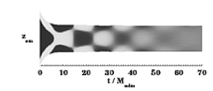
FIG. 7.: We show the time evolution history of the Gaussian curvature for the highly distorted hole ($Q_{0}=1.0$). We plot the curvature as a gray scale using the embedded $z$ value as the $y-$ axis, and $t/M$ as the $x-$ axis. We note that even though the hole is initially very distorted with large curvature, it settles down to a damped oscillatory pattern at later times with a frequency of about $17M$.

In Figs. 8a and 8b we show a similar diagram for the two black hole collision (Misner $\mu=2.2$) evolved in “Class I” coordinates. At late times, $\kappa$ has an appearance similar to that shown by the highly distorted case discussed above. At early times, there are two separate black holes whose horizons are about to merge. The surfaces are most highly distorted along the caustic line, and the Gaussian curvature is largest there. In Fig. 8a we show the entire history of $\kappa$ for this system. We see that in the early times, before coalescence, the Gaussian curvature is very high near the coalescence point. ($\kappa$ is in fact singular on the EH at the caustic; we show the curvature very close to the caustic). In Fig. 8b we show the early time behavior, so the details of the curvature can be seen around the coalescence point.

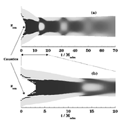
FIG. 8.: We show the time evolution history of the Gaussian curvature for the 2BH collision (Misner $\mu=2.2$). In Fig. (a) we show the entire history of the horizon curvature, and note the repeated oscillation pattern, as in Fig.7, here with a more complicated pattern, but still with a frequency of about $17M$. In Fig. (b) we show the early time behavior of the system, seeing the strong curvature near the systems cusp as the holes come together. We note that the line of caustics is the region inside the two holes before coalescence, as indicated by the arrows.

4 Embedding Diagrams and Embedding Histories

The use of embedding diagrams to study the intrinsic geometry of spacetimes is not new in relativity. It is a particularly useful way to study a curved 2D surface on a constant time slice. The embedding technique creates a fictitious 2D surface in a flat 3D Euclidean space with the same geometric properties as the original 2D surface in the curved 3D space. This technique has been described fully in Ref. [31], where it was used to study AH surfaces. We follow the same embedding approach here.

We can perform a non-trivial test of our embedding treatment by embedding the analytic Kerr horizon, and comparing this horizon with the embedding diagrams predicted in Ref. [27]. For high-rotation Kerr black holes ($a/M>\sqrt{3}/2$), it is not possible to embed the horizon around the pole. In Fig. 9 we show how our EH finder finds and embeds the correct analytic horizon up to the $\theta$ value where the embedding no longer exists.

FIG. 9.: We compare the embedding of the Kerr horizon from our horizon finder with the known embedding for the value $a/M=0.877$, at which the entire horizon cannot be embedded into flat space. We notice the agreement between our finder, the diamonds, and the known solution, the line.

In Fig. 10a-10c we show a time sequence of the embedding diagram for the black hole studied in Fig. 5. In Fig. 10d we show the EH and Schwarzschild embeddings, where both embeddings are normalized by the horizon mass. This normalization removes the spurious area growth caused by errors in the numerical spacetime, as seen in Fig. 2, from our horizon embeddings. In Fig. 10a we see that the initial embedding is very prolate, in concordance with the large value of $C_{r}$ shown in Fig. 5 at $t=0$. We also note that the final state is indeed a Schwarzschild-like horizon, namely a spherical black hole characterized solely by its mass.

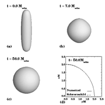
FIG. 10.: We show a sequence of embedding diagrams for an EH distorted by a large amplitude Brill wave. Even though the horizon geometry is very non-spherical at $t=0M$, as demonstrated by the cigar shaped event horizon, the system quickly becomes fairly spherical, as shown in the time snapshots in figures (a), (b), and (c), and also in Fig.5, which corresponds to this system. In Fig. (d) we see that the late time horizon is essentially a Schwarzschild horizon, as it has settled down to a sphere with radius $2M$.

In Figs. 11a-11d we show a time sequence of embedding diagrams of the EH for a Bowen and York, rotating black hole [32, 25], with angular momentum $J=15$, evolved by a code described in Ref. [8]. We see from Fig. 11a that the initial EH is quite spherical (We make the front $45^{\circ}$ of the horizon transparent to facilitate viewing, hence the “pacman” appearance of the horizon). The Bowen and York construction differs from that of a stationary Kerr hole, so this data set can be regarded as containing a gravitational wave that makes the initial black hole horizon more spherical than the oblate pure Kerr hole. At $t=12.4M$ into the evolution, as shown in Fig. 11b, the embedding has a shape reminiscent of a napkin holder; the top and bottom sections of the horizon cannot be embedded as they have negative curvature at the axisymmetric pole, and therefore cannot be represented in a Euclidean space. At this instant in time, the extent of the unembeddable region is near a maximum. Fig. 11c shows the geometry at a later time, as the horizon settles down towards its Kerr form. Fig. 11d shows a quadrant of the EH embedding at time $t=45M$. At this time, the hole has settled down to the Kerr form, in accordance with the no hair theorem [21]. The shape of the EH is to high accuracy the same as that of an analytic Kerr hole of $a/m=0.877$, the embedding of which is plotted as a dotted line for comparison with the numerical result. We note that the value of $a/m=0.877$ is the value of the rotation specified in the initial data solve (a $J=15$ Bowen and York hole), and that this result is still observed late in the evolution. This is physically required, as an axisymmetric system cannot radiate angular momentum. The fact that our horizon finder confirms this late time behavior is a strong verification of the accuracy of our methods. Notice that there is still a region of the horizon that cannot be embedded, as the horizon for such rapidly rotating black hole is “too flat” for Euclidean space, and the regime in which the EH cannot be embedded matches the region for a Kerr EH, as was also shown in Fig. 9.

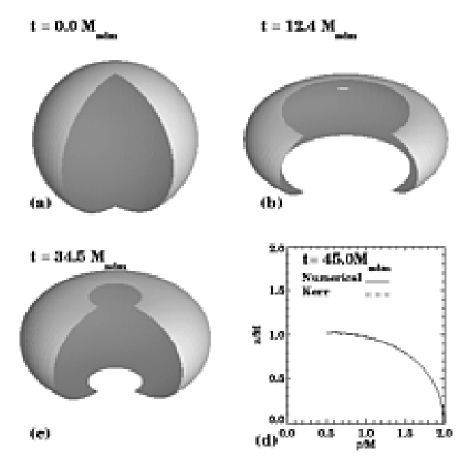
FIG. 11.: We show a sequence of embedding diagrams of the EH for a Bowen and York rotating black hole, with angular momentum $J=15$ ($a/M=0.877$). We show snapshots of the horizon at (a) time $t=0$ (b) time $t=12.4$, and (c) time $t=34.5$. To allow clearer visualization of the region where the embedding fails, we make the front $45^{\circ}$ of the horizon transparent, hence the “pacman” appearance of the holes. We note that, at late times, the system approaches the analytic Kerr embedding.

In Figs. 12a–12d we show four snapshots of the embedding of the EH for the two black hole head-on collision case generated with the Čadež coordinate system for $\mu=2.2$. Fig. 12a shows the embedding of the EH on the initial, time symmetric slice ($t=0$). We see the two individual black holes, with cusps on each horizon on the $z-$axis. In Fig. 12b we show the embedding at time $t=5.4$, shortly after the merging of the two holes. In Fig. 12c we see the late time spherical behavior of the horizon, despite the system’s tumultuous beginnings. In Fig. 12d, we compare the embedding of the EH at $t=80M$, shown as a solid line, to the horizon of a Schwarzschild hole with the appropriate mass, shown as a dashed line (once again, we normalize our final embedding by the final area). Again we see the no hair theorem at work, in that the initial condition with no charge and no angular momentum settled down to a black hole completely described by its single parameter, $M$.

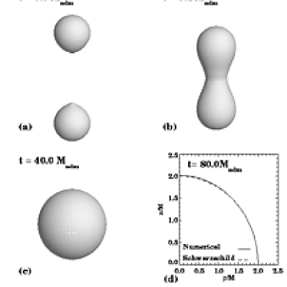
FIG. 12.: We show a sequence of embedding diagrams of the EH for the two black hole head-on collision case at (a) time $t=0$ (b) time $t=5.4M$, and (c) time $t=40.0M$. The simulation here was generated with the Čadež code. We note that at late times, as shown in (d), the system approaches the appropriate Schwarzschild hole, as expected.

To bring out the dynamics of the horizon evolution, it is useful to show the “embedding history diagram” of the horizon instead of a series of snapshots. In Fig. 13, we show the evolution of the embedding in time for the two black hole case just discussed. In this diagram the $\phi$ direction has been suppressed, i.e., we stack up $\phi=\mathrm{const}$ cross sections of the 2D embeddings from various times to create a continuous, 2D embedding history diagram. We note that this figure is not a spacetime diagram, in that the $(\rho,z)$ space away from the horizon surface has no physical or mathematical connection to the curved $3+1$ spacetime. However, these embedding history diagrams are a convenient and effective method for showing the evolution of the embedding of the event horizon surface in coordinate time ($t$) in the fictitious Euclidian ($\rho,z$) space. This figure shows the geometry of the individual holes as they approach each other, with a cusp on each horizon. The distance between the holes before the merger, which is not prescribed in the embedding process for data generated in the Čadež coordinates, is chosen to keep the embedding history diagram smooth. After the merger, one can (barely) see the oscillation of the final horizon, which occurs at the normal mode frequency of the final black hole. In this diagram we also show the evolution of various horizon generators (photons moving normal and tangent to the horizon) as lines on the surface. The determination and use of these generators will be discussed in detail in the next section.

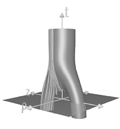
FIG. 13.: We show the embedding history diagram of the two black hole collision generated with the Čadež code. This diagram, the famous “pair of pants” diagram, shows a time history of the embedding of the horizon by stacking consecutive embeddings on top of each other in time. The lines on the surface show the paths of the horizon generators, and shows them leaving the surface at the crossover caustic, as will be discussed below.

Another interesting embedding history diagram is shown in Fig. 14. Here we show the embedding of the equator of the horizon of a Bowen and York black hole from Fig. 11. We see the equator bulge out and then back in, as the hole becomes more and less prolate (the total area increases in time). As discussed in Sec. IV we embed the equator since it allows us to show the generator motion in the $\phi$ direction.

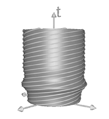
FIG. 14.: We show the embedding history diagram for the case of a distorted Kerr black hole. Here we suppress the $\theta$ direction, and embed only the equator at all $\phi$ values. Although the spacetime is axisymmetric, so there is no $\phi$ variance, this embedding demonstrates the rotation of the generators in the $\phi$ direction as the system evolves in time. This diagram is a numerical construction of the “barber pole twist” diagram.

C Numerical Convergence of the Horizon Measures

The study of numerical convergence is important for any numerical treatments based on finite differencing, and we discuss it for each of our results here. We give a brief overview of numerical convergence here, but for a more detailed discussion, see Refs. [33, 34]. To avoid confusion with Paper I, we emphasize that the numerical convergence we discuss here is the usual convergence rate of our numerical results depending on grid resolution. It is a completely different phenomenon than the physical convergence discussed in Sec. II and in Paper I, which is a physical attraction of null surfaces to the horizon independent of numerical treatment.

Given three solutions to a discretized equation, $L$, $M$, and $H$ at resolutions $\Delta x$, $\Delta x/q$, and $\Delta x/q^{2}$, the convergence exponent is defined as

$$\sigma=\frac{\log\frac{L-M}{M-H}}{\log q}$$ (11)

where $-$ is simple subtraction for numbers, and a combination of interpolation onto a common grid and reduction via a norm operator for fields. The measure $\sigma$ indicates that the error in a numerical solution is of order $\Delta x^{\sigma}$.

In Fig. 15 we show the numerical convergence exponents of the horizon area $A$ and ratio of circumferences $C_{r}$ in a slightly distorted single black hole evolving in time ($Q_{0}=0.1$, $\eta_{0}=0$, $\sigma_{0}=1.0$, $n=2$). We choose this case for our convergence studies since the spacetime is quite accurate so effects of numerical error in the background spacetime are minimized, and we can directly test our horizon treatments (We see similar convergence results for all the spacetimes discussed here; since we have not assumed the Einstein Equations hold in any of our analysis so far, constraint violations in the spacetime will not affect the convergence of the system, although they could in principle cause the horizon analysis to converge to a non-physical result). The convergence study is made by keeping the spacetime resolution fixed in all runs and adjusting only the number of points which represent the horizon. We use an interpolator of order equal to or higher than our evolution method on a numerical grid of data.

We see that the measures $\mathcal{A}$ and $C_{r}$ converge at second order as expected. These quantities are simply measures of the interpolated metric and the surface (evolved with a second order MacCormack method) so any result below second order would signify an error.

Additionally, we measure (but do not show) the average convergence of the $z$-coordinate of the embedding over the entire surface (In the embedding procedure, only the $z$-coordinate is integrated; The $\rho$-coordinate is exactly given as a function of $z$ and the metric). The embedding converges at first order. This is to be expected, since we use a first order integration over the derivative of the surface to form the embeddings. Since the embedding is only measured, not evolved, this first order nature is satisfactory. We note that using a higher order integration scheme would not substantially improve the accuracy of our embeddings, since we cannot remove integrals over derivatives of the surface from our embedding procedure.

FIG. 15.: We show the time evolution of the convergence exponent of $A$ and $C_{r}$ in the low amplitude gravitational wave plus black hole spacetime. We note second order convergence throughout the entire run, and that the convergence rate of $C_{r}$ has (small) spikes associated with an oscillatory function, while that of $A$ does not.

IV Horizon Generators

We have already seen examples of generators of the horizon in several of the above figures. In this section we show that the horizon generators can be located in a numerical spacetime using information already constructed in our surface-based horizon finder. We will use these generators to study the motion and dynamics of black hole event horizons.

A Formulation

The EH is generated by null geodesics. With the EH given by $f(t,x^{i})=0$, the null geodesics that generate the surface satisfy

$$\frac{dx^{\alpha}}{dt}=A(x^{\mu})g^{\alpha\beta}\partial_{\beta}f,$$ (12)

where $A(x^{\mu})$ is a scalar function of the four coordinates. Notice that in terms of $f$, the generators satisfy a first order equation, rather than the more complicated second order geodesic equation. We choose the normalization $A(x^{\mu})$ to be

$$A(x^{\mu})=\frac{1}{g^{t\beta}\partial_{\beta}f}$$ (13)

so that the null vector tangent to the null geodesics is given by

$$\ell^{\mu}=(1,\frac{g^{i\beta}\partial_{\beta}f}{g^{t\alpha}\partial_{\alpha}f}).$$ (14)

Notice that with this choice, the null geodesic is not affinely parameterized, but instead, adapted to the global time coordinate $t$ used in the numerical calculation of the spacetime itself.

One important advantage of determining the null generator using Eqs. (12) and (13) is that in this formulation, the trajectories obtained are guaranteed to lie on the EH. This is in contrast to numerically integrating the second order geodesic equation directly. As shown in Paper I, integration of the geodesic equation directly can lead to spurious tangential drifting effects which can significantly affect the position of the horizon generators. This difference can lead to errors of interpretation, as described in Paper I. The importance of obtaining accurate trajectories of the horizon generators is clear. Generators of the horizon contain all the information of the dynamics of the EH. The entire membrane formulation described Sec. V is based on these trajectories. Thus, inaccurate location of the generators due to tangential drifting can make analysis of the horizon dynamics via the generators impossible.

B Analytic Kerr as a test case

We briefly study the motion of generators in the analytic Kerr case. In this case, a generator will rotate in the $\phi$–direction on the horizon with a rate

$$\frac{d\phi}{dt}=\frac{a}{2M^{2}+2M(M^{2}-a^{2})^{1/2}}.$$ (15)

In Fig.16 we show $d\phi/dt$ for various Kerr spacetimes. We measure the $\phi$ location of the horizon generators, numerically differentiate in time, and show the result as solid black diamonds. We compare these results with the analytic result, Eq. 15, shown as a solid line. We note the results agree with the analytically expected value.

FIG. 16.: We show horizon generator angular velocity, $d\phi/dt$ for a $M=1$ black hole with values of $a/M$ between 0 and 1 as solid diamonds. We compare these results with the analytic value, shown as a solid line. We note the excellent agreement

C Horizon Generators in Dynamical Spacetimes

We now apply these techniques to the study of the trajectories of the horizon generators for three numerically constructed dynamical spacetimes.

We first consider the low amplitude Brill wave plus black hole spacetime considered above ($Q_{0}=0.1$). In this spacetime we expect a non-spherical evolution in the generators. Rather than just moving radially, as the generators would in a dynamically sliced spherical spacetime, we also expect some non spherical deflection to be noticeable in the generators. We show this deflection by plotting the difference between the generator angular location, $\theta_{gen}$ and the late time generator location, $\theta_{0}$, versus $\theta_{0}$ itself, evolving in time. Equatorial plane symmetry requires there is no deflection at the equator, and axisymmetry require that there is no deflection at the pole, thus all the generator deflection must occur between the equator and the pole. In the intermediate region, the generators oscillate with a quasi-normal mode frequency with an amplitude dying down at late times. In Fig.17, we show the deflection quantity $\theta_{\rm gen}-\theta_{0}$ evolving in time, and note that the deflection is small, but displays this expected behavior.

FIG. 17.: We show the angular deflection of generators for a horizon with a low amplitude brill wave initially incident on a black hole. We show the deflection by plotting the angular location of the generators, $\theta_{\rm gen}$ minus their late time position, $\theta_{0}$, versus their late time position, $\theta_{0}$, evolving in time for all generators. From the figure it is clear that the angular deflection occurs away from the equator and pole, as is obvious from simple symmetry arguments.

In Fig. 14, the “Barber Pole Twist” diagram, we have seen the $\phi$ motion of the generators in Kerr-like spacetimes. In Fig.18, we plot the quantity $d\phi/dt$ of the photons versus time. We see that they settle down to a constant value at late times, with

$$\frac{d\phi}{dt}(t=50M)=0.293.$$ (16)

This is to be compared to the analytic value of 0.296 given by Eq. (15) with $a/M=0.877$, denoted by the dashed line in the figure. We see that the measured value at $t=50M$ differs from the analytic value by about $1\%$, which demonstrates that the hole is settling down to a Kerr black hole at late times, and that the determination of the horizon generators is quite accurate, although late time errors in the numerical spacetime lead to the observed small difference from the expected value in the generator angular velocity.

FIG. 18.: We plot the generator angular velocity $d\phi/dt$ for a horizon generator on the equator vs. $t$ for the distorted Kerr black hole. We note that, although this quantity is not constant in time, it approaches the analytic value of $0.296$ at late times, as the horizon settles down to its Kerr form.

Turning to the “Pair of Pants” diagram, Fig. 13, which shows the embedding of two colliding BHs, we see that the most interesting feature of the generators is that some of them leave the horizon (going backwards in time) at the inner seam of the pants. There is a line of caustic points on the $z$-axis extending backward from the “crotch” point where the two horizons merge. It is at these points along the caustic line in the history diagram that photons originally travelling in the causal past of null infinity $(J^{-}(\mathcal{I}^{+}))$ join the horizon as generators. As discussed above, only the surface of the horizon has been embedded; the photons that have left the embedding diagram have also left the embedding space, and their paths are only shown to denote their joining the horizon.

In Fig. 19 we show the coordinate location of the generators and horizon surface found using the Čadež code. The EH location at various times is shown by heavy solid lines. The $t=0$ surface is the horizon of two distinct BHs at the initial time, which evolves to a single, merged horizon, shown at $t=3.1M$. We see that generators which start outside the EH (denoted by inward pointing triangles in the figure) move inwards, cross on the $z$-axis, and join the horizon. This crossing of generators of the EH in the two black hole collision is crucial to recent understanding of the structure of the horizon in the Misner spacetime. Further analysis of the nature of such lines of caustics is possible and underway[35]. Coupled with new techniques for evolving multiple black hole spacetimes, our techniques should allow an increase in our understanding of how the generators behave in dynamical multiple black hole spacetimes.

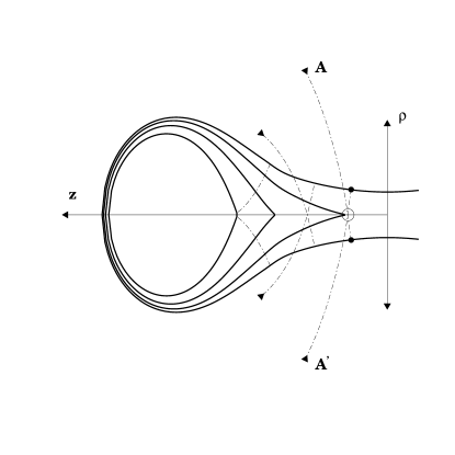
FIG. 19.: In this diagram we analyze the trajectories of the photons before and after they join the horizon for the case of two colliding black holes (Misner $\mu=2.2$). Slices of the horizon are shown at $t=0$, $1.9$, $2.7$, and $3.1M$. We note that generators not originally on the horizon (shown by inward pointing arrows on this figure) cross over each other at a line of caustics on the $z-$ axis and join the horizon as the holes collide. For example, the two photons labeled $A$ and $A^{\prime}$ join the horizon at $t=2.7M$, crossing over at the point shown as an open circle. At time $t=3.1M$ they are on the horizon at the points shown as solid circles. The second black hole is not shown, as the system has equatorial plane symmetry.

D Numerical Convergence of the Generators

We can measure convergence of the generator locations, just as we measured convergence of horizon measures. Since the generator location is an ODE integration with coefficients determined by the surface location and the derivatives of the surface, the appropriate test is to keep the number of generators fixed, while changing the spacing of the surface. We can then measure the differences in generator locations as a function of spacing of the surface and form a convergence measure for each generator, which can then be averaged over all generators.

We show the result of performing this operation on the radial and angular positions of the generators in Fig. 20, using the low amplitude Brill wave plus black hole spacetime considered above. We note that the radial position of the generators (solid line), which is non-oscillatory, converges at second order. However, the angular position (dashed line) has spikes typical of an oscillatory function, but converges below second order. This lower order convergence is due to the principal term in the angular generator position evolution being the (interpolated) derivative of the horizon surface. That is, since we interpolate second order spatial derivatives of the surface for the generator sources, the evolution of the generator angular positions has error terms larger than the $\Delta q^{2}$ terms. This convergence order could possibly be increased by using fourth order spatial derivatives and very high order interpolators.

FIG. 20.: We show the convergence of $r$ and $\theta$ for the horizon generators in the low amplitude Brill wave spacetime. The convergence exponents $\sigma_{r}$ and $\sigma_{\theta}$ are plotted versus time. We note that the radial location of the generators converges at second order, but the angular location converges at somewhat less than second order. This is unsurprising since the evolution equation for generators’ angular location is dominated by an interpolation of the numerical derivative of the horizon surface.

V The Membrane Paradigm

We now turn to a detailed analysis of the information carried by the congruence of horizon generators, and the extent to which this can be used in numerical relativity as a tool to investigate black hole dynamics. The theoretical basis for this study is based on the membrane paradigm (MP) [1]. The MP views the black hole as a 2-surface in a 3-space with the properties of a viscous fluid. In many ways, the EH in a dynamical spacetime is like a soap bubble perturbed by external influences. The MP is particularly valuable in providing an intuitive understanding of how a BH reacts to its surroundings.

There has been much study of gravitational interactions using the MP in quasi-stationary situations [36, 37]. With the advent of numerical identification of the EH and generators described above, we can now start to consider applying the MP to fully non-linear and dynamical spacetimes. With this goal in mind, we demonstrate how to construct the MP quantities on a numerically located EH, and examine the accuracy of these constructions in several testbed spacetimes.

A Formulation

We begin by discussing the MP formalism with the goal of being able to construct MP quantities on our numerically located horizons. The membrane paradigm requires the choice of a time slicing, splitting up spacetime into an “absolute space” and a “universal time”[1]. To apply the MP to numerical relativity, we choose the universal time to be the same as the time coordinate $t$ used in the numerical evolution. This implies that the time coordinate used in the numerical evolution has to be well behaved on the EH. This is the case for all of the black hole spacetimes we have numerically constructed.

We define the four vector $\vec{\ell}$ to be the tangent to the horizon generators, and we normalize it as in Eq. (14) above, with $t$ being considered as the “universal time”. This vector is in the full 4-dimensional space, which we index with Greek letters, $\mu,\nu\ldots=(0,1,2,3)$. On the 2D spacelike section of the EH at constant $t$, we choose spacelike 2D coordinates $\bar{x^{a}}$ which we index with lower case Roman letters, $a,b,\ldots=(2,3)$, which are comoving with the horizon generators, i.e.,

$$\vec{\ell}=\frac{\partial}{\partial t}\Bigg{|}_{\bar{x^{a}}}=\frac{\partial}{\partial\bar{t}}$$ (17)

where $\bar{t}$ is the comoving generator time coordinate (which is identical to the time in the simulation by Eq. (14)). In a coordinate basis, we have the spatial basis vectors

$$\vec{e_{a}}=\frac{\partial}{\partial\bar{x^{a}}}\Bigg{|}_{t}$$ (18)

which are orthogonal to $\vec{\ell}$ by construction. We define the fourth basis vector $\vec{n}$ by

$$\vec{n}\cdot\vec{n}=0$$ (19)

$$\vec{n}\cdot\vec{\ell}=-1$$ (20)

$$\vec{n}\cdot\vec{e}_{a}=0.$$ (21)

The induced metric on the 2D horizon section is

$$\gamma^{H}_{ab}=e_{a}^{\mu}e_{b}^{\nu}g_{\mu\nu}.$$ (22)

In the membrane paradigm the description of the dynamics of the horizon is given in terms of the horizon surface gravity $g_{H}$, the shear $\sigma^{H}_{ab}$, the expansion $\Theta^{H}$, and the Hajicek field $\Omega^{H}_{a}$. They are defined as

$$\Theta^{H} = \frac{1}{2}\frac{\partial}{\partial\bar{t}}{\mathrm{l}n}\,{\mathrm{d}et}\,\gamma^{H}$$ (23)

$$\sigma^{H}_{ab} = \frac{1}{2}\left(\frac{\partial\gamma^{H}_{ab}}{\partial\bar{t}}-\Theta^{H}\,\gamma^{H}_{ab}\right)$$ (24)

$$\nabla_{\vec{\ell}}\,\,\vec{\ell} = g_{H}\,\vec{\ell}$$ (25)

$$\Omega^{H}_{a} = -\vec{n}\cdot\nabla_{a}\vec{\ell}$$ (26)

These quantities are dependent on the choice of time coordinate $t$, as they explicitly involve $\vec{\ell}$ in their definition. That is, they are gauge dependent measures of the horizon dynamics. In the formulation of the membrane paradigm given in Ref. [1], a particular time slicing is chosen for a stationary black hole, e.g., a Kerr black hole. In this slicing, without perturbation, $g_{H}$ and $\Omega_{H}$ take on special values while $\Theta^{H}$ and $\sigma^{H}_{ab}$ vanish. For small perturbations about a Kerr horizon, $g_{H}$ and $\Omega_{H}$ are first order slicing dependent. In the formulation given in Ref. [1], time slicings of the perturbed black hole are chosen so that the surface gravity $g_{H}$ remains unchanged in time. In our application of the membrane paradigm to numerical relativity, as we are mostly interested in highly dynamical and fully nonlinear interactions, we do not put such restrictions on the time slicing. Rather, we let the time slicing be determined by the natural choice of the numerical evolution (maximal slicing for most cases presented in this paper). We expect that the new features introduced by different slicings will become familiar when the formulation is used in more black hole studies, and hopefully allow further insight into the slicing conditions and numerical evolutions.

The horizon quantities (23) - (26) satisfy the following:

The “tidal force equation”

$$D_{t}\sigma_{ab}^{H}+(\Theta_{H}-g_{H})\sigma_{ab}^{H}=-C_{a\mu b\nu}\ell^{\mu}\ell^{\nu}\equiv-{\mathcal{E}}^{\mathcal{H}}_{ab},$$ (27)

the “focusing equation”

$$D_{t}\Theta_{H}=g_{H}\Theta^{H}-\frac{1}{2}\Theta_{H}^{2}-\sigma^{H}_{ab}\sigma_{H}^{ab}-8\pi T_{\mu\nu}\ell^{\mu}\ell^{\nu},$$ (28)

and the “Hajicek equation”

$$D_{t}\Omega_{a}^{H}+(\sigma_{a}^{Hc}+\frac{1}{2}\delta_{a}^{c} \Theta_{H} )\Omega_{c}^{H}+\Theta_{H}\Omega_{a}^{H}=$$ (29)

$$(g_{h}+\frac{1}{2} \Theta_{H} )_{,a}-{\sigma_{a}^{Hb}}_{||b}+8\pi T_{a\mu}\ell^{\mu}.$$ (30)

$D_{t}=\perp\ell\cdot\nabla$ is the projection of the covariant derivative along $\ell$ into the horizon section. “$||$” denotes covariant differentiation on the horizon section. $C_{\mu\nu\rho\sigma}$ is the Weyl tensor and $T_{\mu\nu}$ is the energy-momentum tensor.

The comparison of Eqs. (27)-(30) with the evolution equations for a 2D viscous fluid gives meaning to the horizon quantities Eq. (23) - (26). One finds that Eq. (27) describes the response of a fluid to a gravitational tidal field, Eq. (28) describes the energy conservation of the viscous flow, and Eq. (30) is the corresponding Navier-Stokes equation of the fluid flow. The surface density of the mass-energy of the fluid is identified as $-\Theta_{H}/8\pi$, the surface pressure is $g_{H}/8\pi$, and the momentum density corresponds to $-\Omega^{H}_{a}/8\pi$. The dynamics of the EH of a black hole can be understood in analogy to the motion of a fluid on a soap bubble. In the following section, we show how these “fluid” quantities can be constructed for an EH located in a numerical simulation.

B Constructing Membrane Quantities

Once $f(t,x^{i})=0$ is given, we obtain $\vec{\ell}$ as given in Eq. (14) in a straightforward manner. Next, we define the comoving coordinates $\bar{x}^{a},(a=1,2)$ on the horizon section by $(\bar{\theta},\bar{\phi})$. Then we have

$$\vec{e}_{a}=\left(\partial_{\bar{\theta}},\partial_{\bar{\phi}}\right)=\left(\vec{p},\vec{q}\right).$$ (31)

The coordinate components of the two basis vectors can be obtained by

$$\vec{p}=\partial_{\bar{\theta}}=p^{r}\partial_{r}+p^{\theta}\partial_{\theta}+p^{\phi}\partial_{\phi},$$ (32)

where $p^{r}$ is defined to be

$$p^{r} = \frac{\partial r}{\partial\bar{\theta}}$$ (33)

$$= \frac{\hbox{difference in }r\hbox{ for neighboring generators}}{\hbox{difference in }\bar{\theta}\hbox{ for neighboring generators}},$$ (34)

and likewise for $p^{\theta}$, $p^{\phi}$. We use this definition in a discrete fashion, differencing over generator locations, and therefore our basis vectors will always have a discretization error based on the initial spacing of generators in $\bar{\theta}$ space. As the coordinates $\bar{\theta}$ and $\bar{\phi}$ are chosen to be comoving, we have $p^{t}=0=q^{t}$. For the axisymmetric cases considered here, we pick $\phi=\bar{\phi}$ and thus $\vec{q}=\partial/\partial\phi$, the azimuthal killing vector.

The horizon two–metric is then written as

$$\gamma^{H}_{ab}=\left(\matrix{\gamma^{H}_{\bar{\theta}\bar{\theta}}&\gamma^{H}_{\bar{\theta}\bar{\phi}}\cr\gamma^{H}_{\bar{\theta}\bar{\phi}}&\gamma^{H}_{\bar{\phi}\bar{\phi}}}\right).$$ (35)

The individual components are defined by, e.g.,

$$\gamma^{H}_{\bar{\theta}\bar{\theta}}=g_{ij}p^{i}p^{j}$$ (36)

Solving for $\vec{n}$ is particularly troublesome. We use the following, geometrically motivated, method. When we solved for $\partial_{t}f$ in Eq. (3), we solved the quadratic equation choosing the positive root for the outgoing null surface. We could also have chosen the negative root, and found an evolution equation for the ingoing null surface. Let us call the ingoing evolution equation $\partial_{t}^{-}f$, and Eq. (3) $\partial_{t}^{+}f$ temporarily. We will use the notation $\partial_{\mu}^{\pm}f=(\partial_{t}^{\pm}f,\partial_{i}f)$. Thus, we can form two null vectors $\vec{L}$ and $\vec{N}$ as

$$L_{\mu} = (\partial_{t}^{+}f,\partial_{i}f)$$ (37)

$$N_{\mu} = (\partial_{t}^{-}f,\partial_{i}f).$$ (38)

From Eq. (2) it is clear that both $\vec{L}$ and $\vec{N}$ are null, and that $\vec{L}$ is simply $\vec{\ell}$ with a different normalization.

However it is also clear that $\vec{N}\cdot\vec{e}_{a}=0$. To see this, recall that $\vec{e}_{a}$ has only spatial components, so

$$N_{\mu}e_{a}^{\mu}=e_{a}^{i}N_{i}=e_{a}^{i}\partial_{i}f=e_{a}^{i}L_{i}=L_{\mu}e_{a}^{\mu}=0$$ (39)

since $\vec{L}$ is proportional to $\vec{\ell}$ which is orthogonal to $\vec{e}_{a}$ by construction.

So now all that remains is to find a normalization such that $\vec{n}\cdot\vec{\ell}=-1$. This is straightforward. Since $\vec{\ell}=\vec{L}/A(x^{u})$, using Eq. (13) it is clear that

$$\vec{N}\cdot\vec{\ell}=\frac{g^{\mu\nu}\partial_{\mu}^{+}f\partial_{\nu}^{-}f}{g^{t\alpha}\partial_{\alpha}^{+}f}\equiv B(x^{\mu})$$ (40)

and so we can define $\vec{n}$ by rescaling $\vec{N}$ by $B(x^{\mu})$,

$$\vec{n}=-\vec{N}/B(x^{\mu}).$$ (41)

We note we can use Eq. (19) to measure how accurately $\vec{n}$ and $\vec{\ell}$’s orthogonality with $\vec{e}_{a}$ is maintained.

Once the horizon 2–metric $\gamma^{H}_{ab}$ and full set of comoving vectors, $(\vec{l},\vec{n},\vec{p},\vec{q})$ are obtained, we can form the expansion, shear, and Hajicek Field via Eq. (23) - (26). From Eq. (26), the surface gravity is

$$g_{H}=\Gamma^{t}_{\mu\nu}\ell^{\mu}\ell^{\nu},$$ (42)

for our particular parameterization of $\vec{\ell}$.

There are several terms in the definitions of the membrane quantities which require careful numerical and analytical treatment in order to be evaluated in our framework. In particular, in order to evaluate the horizon quantities accurately, we must be able to evaluate $\partial\gamma_{ab}/\partial\bar{t}$, preferably without taking numerical time derivatives. From Eq. (36), the horizon 2–metric $\gamma$ has two types of terms, those due to the comoving basis vectors $\vec{p}$ and $\vec{q}$, and those due to the spacetime 4-metric, $g_{ij}$. Thus using the chain rule to evaluate $\partial\gamma_{ab}/\partial\bar{t}$ will yield terms like $\partial g_{ij}/\partial\bar{t}$ and $\partial p^{i}/\partial\bar{t}$.

The derivatives along the generators of the spacetime metric can be evaluated using the metric evolution equations. We note that this is the first point we have used the evolution equations for $g_{ij}$, and therefore the accuracy with which our spacetime obeys these evolution equations enters can enter into our quantities. In other words, if the relationship between $\partial_{t}g$ and $2\alpha K$ is only obeyed to a given order, we cannot expect our quantities which use this relationship to be obeyed at a higher order. By virtue of $\ell^{t}=1$,

$$\frac{\partial g_{ij}}{\partial\bar{t}}\equiv\ell^{\mu}\partial_{\mu}g_{ij}=-2\alpha K_{ij}+D_{i}\beta_{j}+D_{j}\beta_{i}+\ell^{k}g_{ij,k}$$ (43)

where $K_{ij}$ is the extrinsic curvature of the 3 surface. $K_{ij}$ and $g_{ij}$ are both readily available in the numerically constructed spacetime.

We can find the terms $\partial p^{i}/\partial\bar{t}$ by commuting partial derivatives. Namely,

$$\frac{\partial p^{i}}{\partial\bar{t}}=\frac{\partial}{\partial\bar{t}}\frac{\partial x^{i}}{\partial\bar{\theta}}=\frac{\partial\ell^{i}}{\partial\bar{\theta}}.$$ (44)

The time derivative of $\vec{p}$ is the spatial derivative of $\vec{\ell}$. We can evaluate the spatial derivative of $\vec{\ell}$ with a single time slice finite difference of our surface and surface quantities, and thus find the required time derivatives. To summarize, expanding the time derivative of the horizon metric using the chain rule, and using the above two techniques, we can find the $\partial\gamma_{ab}/\partial\bar{t}$ terms in a single time slice.

Thus, we have a method for finding the four horizon quantities which describe the kinematics of the horizon surface. This method is contained entirely in a single 3-slice. We should note that it is also possible to create the membrane quantities in a direct fashion using numerical derivatives in time to evaluate the expansion and shear. We call this the “time difference” evaluation of the expansion, as opposed to the “single slice” evaluation. We find that the single slice method invariably gives smoother and more accurate data for the membrane quantities than the time difference method.

An additional difficulty comes in evaluating the horizon equations, Eq. (27)-(30). Two terms pose a difficulty there, $D_{\bar{t}}Z_{a}$ and ${{\sigma_{a}}^{b}}_{||b}$, where $Z$ is any tensor on the horizon. Luckily, we only need to evaluate these terms as a check; we do not use the horizon equations in our evolution. Thus we can use first order accurate methods to evaluate these if need be.

We first turn our attention to $D_{\bar{t}}Z_{a}$. First we introduce a Christoffel symbol for the $(\bar{t},\bar{\theta},\bar{\phi})$ coordinates (e.g., the null horizon 3-surface in co-moving coordinates, which we will here index with $(q,r,\ldots)$). We denote this as ${}^{(3)}{\Gamma^{q}}_{rs}$. We find

$$D_{\bar{t}}Z_{a}=\frac{\partial Z_{a}}{\partial\bar{t}}-{}^{(3)}{\Gamma^{q}}_{a\bar{t}}Z_{q}.$$ (45)

The horizon “3-metric”, $\gamma_{qr}$ is simply given by $\gamma_{ab}$ if $q,r\not=\bar{t}$ and $0$ elsewhere. Thus ${}^{(3)}{\Gamma^{q}}_{rs}$ can be simply evaluated as

$${}^{(3)}{\Gamma^{q}}_{a\bar{t}} = \frac{1}{2}\gamma^{qr}\left(\gamma_{ra,\bar{t}}+\gamma_{r\bar{t},a}-\gamma_{\bar{t}a,r}\right)$$ (46)

$$= \frac{1}{2}\gamma^{qb}\gamma_{ab,\bar{t}}$$ (47)

Thus we can easily evaluate Eq. (45) as

$$D_{\bar{t}}Z_{a}=\frac{\partial Z_{a}}{\partial\bar{t}}-\frac{1}{2}\gamma^{bc}\gamma_{ba,\bar{t}}Z_{a}.$$ (48)

The only term which we cannot calculate in a single slice is $\partial Z_{a}/\partial\bar{t}$, but we can simply calculate that by storing the quantity $Z_{a}$ at three time steps and then use a centered time derivative to evaluate the term at the middle step after all three steps are taken.

The term ${{\sigma_{a}}^{b}}_{||b}$ is evaluated directly, e.g.,

$${{\sigma_{a}}^{b}}_{||b}={{\sigma_{a}}^{b}}_{,b}+{}^{(2)}{\Gamma^{b}}_{cb}{\sigma_{a}}^{c}$$ (49)

and the 4 independent non-zero terms of ${}^{(2)}{\Gamma^{a}}_{bc}$ are evaluated directly from spatial derivatives of the horizon 2-metric.

C Test and Applications of MP Quantities

In this section we apply the membrane quantities to a set of testbed analytical and numerical black hole spacetimes that have been computed using codes described in Refs. [5, 8]. Our aim here is to probe whether these tools can be used in a practical way to explore the dynamics of black hole horizons in numerically generated spacetimes. We will consider the physics of these quantities, for a set of interesting spacetimes, in a future paper.

1 Flat space

Flat space in Minkowski coordinates,

$$ds^{2}=-dt^{2}+dr^{2}+r^{2}d\Omega^{2}$$ (50)

allows us to test our expressions for $\Theta$ against easily understandable analytic solutions. Although flat space has no EH, it does have null surfaces, and our construction carries over to them.

Most notably, we know that for spherical null surfaces in flat space, the expansion of a sphere of radius $r$ is

$$\Theta=\frac{1}{\cal A}\frac{\partial{\cal A}}{\partial t}=\frac{2}{r}.$$ (51)

since in flat space, ${\cal A}=4\pi r^{2}$ and $\partial r/\partial t=c=1$. Using this relationship, we can trivially check our expressions for $\Theta$. Additionally, we can form $\partial{\cal A}/\partial t$ from integrals of the expansion, which carries over into the dynamical black hole case, where we can compare this integral of $\Theta^{H}$ with a numerically calculated $\partial A/\partial t$. Evaluating the expansion in flat space gives the expected answer.

2 Analytic Schwarzschild

We next turn to the analytic Schwarzschild spacetime described in standard coordinates,

$$ds^{2}=\left(1-\frac{2M}{r}\right)dt^{2}+\frac{dr^{2}}{\left(1-\frac{2M}{r}\right)}+r^{2}d\Omega^{2}.$$ (52)

In this spacetime, the expected results are that the generators and surface will be attracted backwards in time towards the true horizon (at $r=2M$), that $\Theta_{H}$, $\sigma^{H}_{ab}$ and $\Omega^{H}_{a}$ approach zero exponentially as the surface approaches the true horizon, and that $g_{H}$ approaches the analytic value of $1/2M$. Moreover, we can check that relationship between the integral of the expansion and the area change holds in this spacetime by numerically differentiating the horizon area, which allows another test of our expressions. These relationships are obeyed.

In analytic Schwarzschild we can trivially evaluate the above expressions for $\vec{\ell}$, $\Theta$ and $g_{H}$ on an arbitrary null sphere of radius $r$ to find

$$\vec{\ell} = \left(1,1-\frac{2M}{r},0,0\right),$$ (53)

$$\Theta = \frac{2}{r}\;\ell^{r}=\frac{2}{r}\left(1-\frac{2M}{r}\right),$$ (54)

$$g_{H} = \frac{2M}{r^{2}}\;\frac{\ell^{t}\ell^{r}}{1-\frac{2M}{r}}=\frac{2M}{r^{2}}.$$ (55)

Note that $\ell^{r}$ and $\Theta$ vanish on the horizon ($r=2M$) as expected, and $g_{H}$ takes the value $1/2M$. We check these relationships for surfaces away from the horizon and we see that our surfaces give the analytic results for all null spheres in the spacetime.

Additionally, each of the horizon equations, Eq. (27)-(30) should be obeyed in this spacetime. We evaluate only the focusing equation violation, however, since the tidal force equation contains the electric part of the Weyl tensor, ${\mathcal{E}}^{H}_{ab}$, which causes this equation not to be a check on the membrane quantities alone, and the Hajicek equation is trivially satisfied with a spherically symmetric $g_{H}$ and $\Omega^{H}_{a}=0$.

The vanishing of the focusing equation violation allows us a strong check on our method. Since the focusing equation requires the covariant derivative of the expansion, $D_{t}\Theta$, we expect the focusing equation to be obeyed as accurately as $D_{t}\Theta$ is evaluated. Recall, we evaluate $D_{t}\Theta$ by taking a centered finite difference in time, so we expect the focusing equation violation in our spacetime to converge towards zero at ${\cal O}(\Delta t^{2})$. We test this by finding a surface in the analytic Schwarzschild background first using a Courant factor $\lambda=0.2$ and then $\lambda=0.4$, doubling the time step. We then measure the focusing equation violation in these two runs. If the result is converging towards zero, the focusing equation violation should be four times larger in the $\lambda=0.4$ case. We demonstrate this convergence in Fig. 21 by plotting the focusing equation violation with $\lambda=0.2$ as a line, and by plotting one quarter the focusing equation violation with $\lambda=0.4$ as diamonds. The demonstration that these two sets of data are the same indicates that we are converging towards a surface which satisfies the focusing equations. We note that, as the surface becomes very close to the actual horizon, the focusing equation is zero at levels close to machine precision in both simulations, so convergence can no longer be observed numerically.

FIG. 21.: We show the violation of the focusing equation, $F$, for a given sized time step as a solid line, and one quarter the violation for double the time step as diamonds, for a surface integrated in the analytic Schwarzschild spacetime. The fact that these data are coincident indicates that we are converging towards a null surface which satisfies the focusing equation. The surface in question starts at $r=2.4M$ at $t=30$. The exponential shrinking of the violation is directly due to the exponential approach of the expansion towards zero. Note also that as the focusing equation approaches machine precision levels (here $10^{-14}$) convergence fails, since both quantities are effectively zero.

3 Maximally Sliced Schwarzschild

With the advent of new hyperbolic systems for the Einstein equations [38, 39, 40] and Apparent Horizon Boundary Conditions [24, 10], long time highly accurate one dimensional evolutions of a maximally sliced Schwarzschild black hole are quite readily available, and so we can use these very accurate spacetimes to test our horizon finding method. In this section, we consider a maximally sliced black hole evolved with the eigen-method code described in Ref. [39], which allows long time evolution with exceptionally small error.

We first can test the evaluation of the horizon 2-metric, $\gamma_{ab}$. In the case of no angular generator motion, where the generators are chosen to be identically on the points on which the horizon surface $f(t,x^{i})$ is evolved, the horizon 2-metric $\gamma_{ab}$ and the induced surface 2-metric used to evaluate area and circumferences should be identical. That is, we should get the same answer evaluating Eq. (7) whether we use $\gamma_{ab}$ as defined by Eq. (6) or Eq. (22). Moreover, the vectors $\vec{p}$ and $\vec{q}$ should have components $(0,0,1,0)$ and $(0,0,0,1)$ respectively. We see both of these features to machine precision in the maximally sliced Schwarzschild spacetimes.

Spherical symmetry also leads to a vanishing shear; our expression for the shear vanishes to machine precision. However the expressions for the expansion is non-trivial, and since we have a very small (but non-zero) area growth due to numerical error, we can very accurately measure how well the expansion measures area change.

We choose two trial surfaces for our test, one slightly outside the horizon and one slightly inside, and integrate them backwards in time. As expected from Paper I, these surfaces converge towards each other rapidly, and lock onto the same surface, but have some non-trivial area change, due to the “locking on” process before the surfaces join the horizon, and due to numerical error afterwards. In Fig. 22 we plot $\partial{\cal A}/\partial t$ calculated by differentiating the area reported by the code, and also by integrals over the surface of the expansion. We see that these quantities agree, strongly indicating that our evaluation of the expansion is correct.

FIG. 22.: We show $\partial{\cal A}/\partial t$ evaluated by taking both the numerical derivative of the area calculated by the code, and surface integrals of the expansion found from the comoving horizon two metric. We use a very accurate maximally sliced Schwarzschild spacetime which has a very small, but non-zero, numerical error in the spacetime. We integrate two surfaces, one originally inside and the other originally outside the event horizon. We note the excellent agreement between the two measures of $\partial{\cal A}/\partial t$.

4 Small Distortion Non-rotating Black Hole

We turn to the small distortion Brill wave plus black hole spacetime considered above. We first test if our evaluation of the horizon two metric, $\gamma_{ab}$, gives measures of the horizon geometry which are consistent with the measures discussed in Sec.III B. Since the generators will experience angular deflection, integrals to form areas and circumferences will be over different coordinate locations when using the comoving and induced two metric. Moreover, the measure of the geometry using the horizon two metric will be measured on a non-regular grid in $\theta,\phi$ space (but a regular grid in $\bar{\theta},\bar{\phi}$ space), and will therefore have an additional inaccuracy. Nonetheless, we see good agreement. In Fig.23, we show the difference in evaluating $C_{p}$ (not $C_{r}$) using the comoving and induced two metric in the Brill-wave plus black hole spacetime. We show the difference for 38 and 76 generators, respectively. Note as the number of generators increases (therefore reducing numerical error in the integration over the horizon metric due to generator deflection), the results converge towards the same solution, or the differences converge towards zero.

FIG. 23.: We demonstrate that the generator co-moving metric gives accurate evaluations of the polar circumference, $C_{p}$, in the spacetime with small amplitude Brill waves initially on the throat. We show this by forming $C_{p}^{\mathrm{s}fc}$ from the induced surface metric, and $C_{p}^{\mathrm{g}en}$ from the co-moving generator horizon 2–metric. We taking the difference of the two measures with different numbers of generators used to form the horizon 2–metric. Clearly, as more generators are used the two methods become closer and the differences converge towards zero.

We turn next to the expansion on the horizon. For the physical setup considered here, a gravitational wave incident on a black hole, but with the wave centered at the throat, we expect the horizon to grow at $t=0$, and then as time progresses, become static. This should show up as a positive expansion decreasing towards zero as time progresses. However, we also know that our spacetime has spurious area growth of the horizon due to numerical error in the spacetime, as found in previous studies of the AH. This should appear as a positive, and increasing, expansion at later times. In Fig. 24 we show the expansion for this spacetime, and see exactly this behavior. However, a few features of the expansion should be noted. Firstly, note that at late times, the expansion is not terribly smooth in time. Secondly, note that, near the axis ($\theta=0$) the expansion is somewhat oscillatory. At late time and near the axis the numerically constructed spacetime is less accurate. We see that our membrane paradigm quantities as analysis tools are very sensitive detectors of these errors in the numerically generated spacetime.

FIG. 24.: We show the evolution of the expansion in time for the horizon interacting with a small amplitude Brill wave. Two features are of interest here. First, we note the initial expansion is quite large but drops quickly, as the horizon swallows the initially incident gravitational radiation. This initial growth is concentrated near the equator, as the gravitational wave has a $\sin^{2}\theta$ form. Secondly we note that at later times the expansion is growing, as expected from the spurious horizon growth due to numerical error, and this growth has no angular dependence. We also note a small amount of noise on the horizon near the axis, due to spacetime inaccuracies there.

This detection of error leads us to study how these quantities behave with changing resolution in the construction of the numerical spacetime. In Fig. 25 we take the same wave parameters used above with resolutions of $200\times 54$ and $300\times 80$ to generate two spacetimes. In Fig. 25, we show the area change predicted by integrating the expansion over the 2-surface. We see that, at $t=0$, where area change is caused by infalling gravitational radiation and the spacetime is still quite accurate, both systems give the same result, but at later times, the expansion due to spurious numerical error is considerably larger in the lower resolution spacetime, and the expansion appears to be converging towards zero. In the high resolution spacetime, the expansion is fairly inaccurate near the pole, as the system is very susceptible to axis instabilities, but this noise does not show up in the calculation of area change, as $\sin\theta$ terms in the integral of the expansion kill this contribution near the pole.

FIG. 25.: We study the behavior of the expansion with a moderate and high resolution numerically generated spacetime. At early times when area growth is due to accurately modeled gravitational phenomena, the expansion should be unchanged by adjusting the spacetime. At late times, when area growth is due to spurious numerical error, the area growth should is smaller with a higher resolution simulation, as the spacetime is converging (at roughly second order) towards a zero-area-growth solution.

We next turn to the shear. In this spacetime, we expect a non-zero shear since there is generator motion, but we also expect the shear $\sigma_{ab}$ to be diagonal, since the spacetime is non-rotating and axisymmetric. In Figs. 26 and 27 we plot the evolution of $\sigma_{\bar{\theta}\bar{\theta}}$ and the trace of the shear, ${\sigma_{a}}^{a}$ in time. We note that the shear is largest near the equator, and vanishes on the pole, as symmetry arguments require it must. (There can be no shear at the pole in axisymmetry, only expansion, since shear at the pole would imply a $\phi$ dependence of the generator motion). We also note that the trace of the shear vanishes to machine precision in Fig. 27

FIG. 26.: We show $\sigma_{\theta\theta}$ on the horizon for the low amplitude distortion case considered. We note that there is no shear at the poles, and the shear is maximal near the equator.

FIG. 27.: We show the trace of the shear, ${\sigma_{\theta}}^{\theta}+{\sigma_{\phi}}^{\phi}$ on the horizon for the low amplitude distortion case considered. We note that, even though the shear and the horizon two metric are order unity, this quantity effectively vanishes to machine precision.

Finally, to test the surface gravity, we turn to the focusing equation, which is a complicated combination of the surface gravity, shear, and expansion. If this equation is roughly satisfied in our spacetime, then we have a strong verification that we are indeed measuring the membrane quantities appropriately. We test this by taking the averaged value of the focusing equation violation (or the LHS - RHS of Eq. (28)) over the surface. In Fig. 28 we show these averages evolving in time in our moderate and high resolution spacetimes. We note that the focusing equation violation is small, being substantially smaller than the square of the shear and the expansion. However it is clear that the evaluation of the focusing equation violation is also sensitive to the errors in the numerical spacetime and interpolations. Noise, which is generated from the discrete and inaccurate features of the spacetime, is clear in Fig. 28. However, we also observe that, with more spacetime resolution, the focusing equation violation converges towards zero at approximately second order, as expected.

FIG. 28.: We show the norm of the focusing equation over the surface in the high resolution and medium resolution spacetimes. We note several features. Firstly, this quantity is noisy, but small compared to the square of the shear and expansion, both of which enter into the equation. Secondly, we note that with an increasingly accurate spacetime, the focusing equation converges towards zero at approximately second order.

From the experiments in these two numerical spacetimes we conclude that our construction is appropriate for measuring and generating membrane paradigm type analysis quantities in numerical spacetimes. These quantities are sensitive detectors of error in numerical spacetimes, and they allow us to measure detailed properties of the event horizon and its dynamics.

VI Conclusions

In this paper, we have developed a set of tools with which one can measure and understand the dynamics of event horizons in numerically generated spacetimes. We have shown that standard geometric measures of the horizon are useful tools for understanding horizon dynamics. We have investigated the behavior of the generators of the horizon in several spacetimes, including two black hole spacetimes, where horizons contain caustics, through which generators leave the horizon. Finally we presented a construction which applies the membrane paradigm to numerical relativity. We demonstrated that this construction was effective on analytic spacetimes, and is also applicable to numerically generated spacetimes. We also note that our techniques are applicable to any null surface, so could potentially be useful for studying null surface dynamics in spacetimes without black holes, or away from black holes. We look forward to more accurate dynamical black hole spacetimes, so we can use these quantities for detailed horizon analysis in numerical relativity.

VII acknowledgements

We are most grateful to Kip Thorne for many discussions and for contributing ideas to this work. We are indebted to Peter Anninos for his assistance with the two black hole studies and for many useful conversations. We are grateful to Steve Brandt for providing data for evolved rotating black holes that were discussed in this paper, and for helpful discussions about the Kerr spacetimes. We thank David Bernstein, David Hobill, and Larry Smarr for providing their axisymmetric Black Hole + Brill Wave spacetime. We thank Greg Daues for providing the one-dimensional AHBC spacetime used to create Fig. 2. We thank Carles Bona and Joan Stela for providing the code used in Sec.V C 3. We thank Carsten Gundlach for interesting conversations.

This work used supercomputer facilities at the National Center for Supercomputing Applications (NCSA), Albert Einstein Institute (AEI), and the Pittsburgh Supercomputing Center (PSC). This work was supported by the Albert Einstein Institute, NSF Metacenter Allocation MCA93025, and NSF grants Nos. PHY94-04788, PHY94-07882, PHY06-00567, ASC95-03978 and ASC93-18152. W.M.S. would like to thank the support of the Institute of Mathematical Science of the Chinese University of Hong Kong.

REFERENCES

- [1] Black Holes: The Membrane Paradigm, edited by K. S. Thorne, R. H. Price, and D. A. Macdonald (Yale University Press, London, 1986).
- [2] R. Penrose, Ann. N.Y. Acad. Sci. 224, 125 (1973).
- [3] K. Thorne, in Magic Without Magic: John Archibald Wheeler, edited by J. Klauder (Freeman, San Francisco, 1972), p. 231.
- [4] C. W. Misner, K. S. Thorne, and J. A. Wheeler, Gravitation (W. H. Freeman, San Francisco, 1973).
- [5] A. Abrahams et al., Phys. Rev. D 45, 3544 (1992).
- [6] S. L. Shapiro and S. A. Teukolsky, Phys. Rev. D 45, 2739 (1992).
- [7] P. Anninos et al., Phys. Rev. Lett. 71, 2851 (1993).
- [8] S. Brandt and E. Seidel, Phys. Rev. D 52, 856 (1995).
- [9] P. Anninos et al., Phys. Rev. D 52, 2059 (1995).
- [10] G. E. Daues, Ph.D. thesis, Washington University, St. Louis, Missouri, 1996.
- [11] K. Camarda, Ph.D. thesis, University of Illinois at Urbana-Champaign, Urbana, Illinois, 1998.
- [12] G. B. Cook et al., Phys. Rev. Lett 80, 2512 (1998).
- [13] C. Bona, J. Massó, E. Seidel, and P. Walker, gr-qc/9804052 (1998), submitted to Physical Review D.
- [14] P. Anninos et al., Phys. Rev. Lett. 74, 630 (1995).
- [15] J. Libson et al., Phys. Rev. D 53, 4335 (1996).
- [16] C. Misner, Phys. Rev. 118, 1110 (1960).
- [17] P. Anninos et al., Phys. Rev. D 52, 2044 (1995).
- [18] P. Anninos, S. R. Brandt, and P. Walker, gr-qc/9712047 (1997), submitted to Phys. Rev. D.
- [19] A. Čadež, Ph.D. thesis, University of North Carolina at Chapel Hill, Chapel Hill, North Carolina, 1971.
- [20] R. Matzner et al., Science 270, 941 (1995).
- [21] S. W. Hawking and G. F. R. Ellis, The Large Scale Structure of Spacetime (Cambridge University Press, Cambridge, England, 1973).
- [22] D. Bernstein, D. Hobill, and L. Smarr, in Frontiers in Numerical Relativity, edited by C. Evans, L. Finn, and D. Hobill (Cambridge University Press, Cambridge, England, 1989), pp. 57–73.
- [23] E. Seidel and W.-M. Suen, Phys. Rev. Lett. 69, 1845 (1992).
- [24] P. Anninos et al., Phys. Rev. D 51, 5562 (1995).
- [25] S. Brandt and E. Seidel, Phys. Rev. D 54, 1403 (1996).
- [26] S. Brandt and E. Seidel, Phys. Rev. D 52, 870 (1995).
- [27] L. L. Smarr, Phys. Rev. D 7, 289 (1973).
- [28] E. Flanagan, Phys. Rev. D 44, 2409 (1991).
- [29] E. Flanagan, Phys. Rev. D 46, 1429 (1992).
- [30] D. Bernstein, D. Hobill, E. Seidel, and L. Smarr, Phys. Rev. D 50, 3760 (1994).
- [31] P. Anninos et al., Phys. Rev. D 50, 3801 (1994).
- [32] J. Bowen and J. W. York, Phys. Rev. D 21, 2047 (1980).
- [33] M. Choptuik, Phys. Rev. D 44, 3124 (1991).
- [34] C. Bona, J. Carot, and J. Massó, In preparation (1998).
- [35] P. Walker, Ph.D. thesis, University of Illinois at Urbana-Champaign, Urbana, Illinois, 1998, in preparation.
- [36] W. M. Suen, R. H. Price, and I. Redmount, Phys. Rev. D 37, 2761 (1988).
- [37] R. H. Price and K. S. Thorne, Phys. Rev. D 33, 915 (1986).
- [38] C. Bona, J. Massó, E. Seidel, and J. Stela, Phys. Rev. D 56, 3405 (1997).
- [39] A. Arbona, C. Bona, J. Massó, and J. Stela, In preparation (1998).
- [40] M. Scheel et al., Phys. Rev. D 56, 6320 (1997).