Three Dimensional Numerical Relativity with a Hyperbolic Formulation

Abstract

We discuss a successful three-dimensional cartesian implementation of the Bona-Massó hyperbolic formulation of the 3+1 Einstein evolution equations in numerical relativity. The numerical code, which we call “Cactus,” provides a general framework for 3D numerical relativity, and can include various formulations of the evolution equations, initial data sets, and analysis modules. We show important code tests, including dynamically sliced flat space, wave spacetimes, and black hole spacetimes. We discuss the numerical convergence of each spacetime, and also compare results with previously tested codes based on other formalisms, including the traditional ADM formalism. This is the first time that a hyperbolic reformulation of Einstein’s equations has been shown appropriate for three-dimensional numerical relativity in a wide variety of spacetimes.

I Introduction and Overview

The young field of three-dimensional (3D) numerical relativity has entered an exciting era. As we review below at some length, strong theoretical and astrophysical motivations have led to increased activity and collaborations among many research groups, and general 3D relativistic problems are being attacked with increasing success. In this paper we present results from a new and very general 3D advanced computer code, which we call “Cactus”[1], designed to study these general problems in a collaborative environment. This is the first in a series of papers on this code and its applications in numerical relativity and relativistic astrophysics. At the same time, the paper is also a follow-up of previous papers in our continuing exploration of hyperbolic formulations of the Einstein equations for numerical relativity[2, 3, 4].

A Motivation

The imminent arrival of data from of the long awaited gravitational wave detectors (LIGO, VIRGO, GEO600, TAMA; see, e.g., Ref. [5] and references therein) has provided a sense of urgency in producing realistic simulations of very strong sources of gravitational waves, which can only be done through the full machinery of numerical relativity. One of the best candidates for early detection by the laser interferometer network is increasingly considered to be black hole mergers[6, 5]. However, the signals are likely to be weak enough by the time they reach the detectors that reliable detection may be difficult without prior knowledge of the merger waveform. These are among the reasons that the NSF-funded Binary Black Hole Grand Challenge Alliance has focused the efforts of numerous US and international groups on developing codes for solving the problem of 3D coalescing black holes (see, e.g, the latest round of papers of the Alliance[7, 8, 9]).

Another important process in astrophysics that requires fully relativistic simulation is neutron star mergers (see, e.g. [10]), which will produce a possibly detectable burst of gravitational waves[11]. These are sometimes considered as sources of gamma-ray bursts [12], and the final state (e.g., a neutron star or black hole) is highly uncertain. Most studies of this process have been Newtonian, but even post-Newtonian correction terms, which are still inadequate to describe the possible formation of a black hole, produce significant changes in the evolution[13]. More relativistic approximations to the Einstein equations produce still quite different (and controversial) results, indicating that the neutron stars may actually form black holes before the merger[10]. The point we wish to make is that the merger process clearly requires a fully consistent relativistic treatment, which provides another motivation for development of powerful and general numerical codes to solve the full set of Einstein equations, in this case coupled to the relativistic fluid equations. This research area is a particular application for which Cactus is being developed, although we will present only tests of the vacuum part of the evolution system in this paper.

Astrophysics aside, there are of course purely theoretical reasons to develop robust 3D solvers to Einstein’s equations. As general relativity is one the fundamental theories of physics, it needs to be better understood in its most nonlinear regimes, which are usually the most difficult to probe. Again, numerical treatment of the full set of Einstein equations is one of the main tools for studying the theory in such regimes, and has already led to the discovery of unexpected phenomena, such as critical phenomena in black hole formation[14] (see Ref.[15] for a recent review), which has now been seen in spacetimes containing scalar fields, fluids, and even in pure vacuum, gravitational wave spacetimes. Most of these studies have been carried out in 1D or in rare cases in 2D[16], but little is known about the 3D behavior[17].

Unfortunately, despite all of these motivations for 3D numerical relativity, and the best efforts of many groups around the world, progress has been slower than hoped and expected. One of the reasons for this is the the sheer complexity of the Einstein equations in 3D, coupled with the immense computational needs for solving them. For example, an enormous amount of memory and time on the order of one CPU day on a Teraflop computer will be required to produce a single, highly resolved simulation of 3D black hole spiraling coalescence (see Ref. [18] for a review). Developing well tested software that simultaneously solves the Einstein equations, takes advantage of high performance parallel computers, and can be effectively used by the large number collaborators needed to develop algorithms is a challenging software engineering problem in its own right.

However, the problems of 3D numerical relativity run far deeper than computation and code development. Given a sufficiently large computer and perfectly debugged code, problems like coalescing black holes or neutron stars would still not be solvable today, because of important theoretical and algorithmic problems still to be addressed. Perhaps the best example to illustrate these problems is that of a spacetime containing black holes.

The presence of a singularity inside the black hole and the weak field zone far from the hole gives rise to an extreme dynamic range. Singularity avoiding slicings effectively keep time slices from hitting the singularity, but lead to pathological time slices that create huge gradients near the black hole horizon which cannot be resolved, especially in 3D[19, 20]. Such gradients lead to numerical instabilities with the standard formulations of the equations, often causing codes to crash in the interior well before the desired evolution can be carried out in the radiation zone. Although the characteristic time necessary to obtain accurate waveforms for the inspiral and merger of two black holes is on the order of thousands of $M$ (see, e.g, Ref.[9]), even state-of-the-art black hole collisions in axisymmetry (2D)[21, 22] can only be evolved for hundreds of $M$. (We will use units $c=G=1$ throughout this paper, so time and spatial units for black hole simulations are in terms of the black hole mass $M$.)

Success in evolving black holes in 3D has been mixed. Partial successes include colliding, equal mass black holes in 3D [18], and waveform extraction of distorted 3D black holes[23, 24, 25]. In both cases the system is evolved successfully for tens of $M$ and although this would be completely insufficient for the black hole coalescing problem, it is enough time to study the waveforms produced in the ring-down phase. As verified by comparison with perturbation theory and axisymmetric simulations, these 3D simulations can produce highly accurate waveforms, but they ultimately crash both due to the “grid stretching”[26] effects created by singularity avoiding slicings and due to poor outer boundary conditions.

One approach to understanding the expected waveforms that avoids these problems is to solve the linearized equations describing black hole gravitational wave interactions. This approach has proven to be remarkably robust in comparisons with a range of presently feasible fully nonlinear simulations of distorted and colliding black hole spacetimes [25, 27, 28, 29, 30, 31], but it does not solve the general coalescence problem. Related studies of a direct 3D integration of the perturbation equations show that even such a simple linear problem is very demanding, having inner and outer boundary difficulties [32] that can be overcome through the machinery of adaptive mesh refinement [33, 34, 35].

The problem of dealing with singularities, grid stretching, and inner boundaries may be ultimately solved by the so-called AHBC (apparent horizon boundary conditions)[36, 37, 38, 39, 40, 8], which are basically ingoing conditions on appropriate quantities evolving near the black hole horizon coupled with appropriate gauge conditions. But other gauge problems may still lead to large gradients as coordinates are sheared and squashed during the evolution. Hence much research into appropriate gauge conditions for such dynamic spacetimes is needed. Even in very weak wave spacetimes, gauge problems can cause numerical codes to develop pathologies and crash as coordinates evolve out of control[41, 42, 43]. Recent developments shed new light into the mathematical understanding of these coordinate problems and gauge pathologies in general[44, 45]. Furthermore, in order to resolve the inner, strong field region near the black holes, the outer boundary is generally placed uncomfortably close to the hole, where spurious signals or reflections which propagate inward may be generated due to inappropriate boundary conditions, masking the true physics taking place in the interior (for a recent discussion, see Ref.[7]).

Despite these difficulties, there has been considerable progress in evolving dynamical black hole spacetimes in the last year. Brügmann[46] recently demonstrated that it is possible to see some form of gravitational radiation from numerically constructed true 3D black holes with spin and momentum. Unfortunately, these feasibility studies seem to indicate that current techniques have face more severe difficulties with these highly dynamical systems, and cannot yet provide useful information for realistic gravitational wave astronomy [46]. The Grand Challenge Alliance has developed outer boundary conditions which appear to allow accurate outgoing wave boundary conditions in three dimensional numerical relativity [7]. Moreover, using causal differencing and a careful inner boundary treatment, the Alliance has been able to transport a black hole several black hole radii across a grid [8]. Work by Daues and collaborators has allowed single black holes to be evolved beyond 100M using dynamically determined gauges [40]. However, none of these treatments have shown, to date, the ability to produce a long time stable evolution for colliding or highly distorted black holes in three dimensions, and many difficult problems remain to be solved.

Another very recent approach to 3D black hole evolution that completely avoids the problems of grid stretching is characteristic evolution, which has successfully evolved 3D rotating and distorted black holes for essentially unlimited time periods ($t\approx 60,000M$[47, 9]). These spectacular results are achieved by using an ingoing characteristic foliation of the black hole spacetime, using the horizon as an inner boundary. However, it is not clear yet if this method will be viable for evolution of very highly distorted or colliding black holes, where focusing of ingoing light rays may create caustics, leading to a breakdown of the foliation. Also, ironically, the method is presently most successful when a black hole is present, creating an $S^{2}\times R$ topology; dealing with the so-called $r=0$ problem is difficult for any formulation of the Einstein Equations, and is avoided by using cartesian grids in the standard 3+1 formulations, but the characteristic method cannot use cartesian grids, and would therefore have to face this problem in the absence of a black hole (e.g., for the coalescence of neutron stars). Nonetheless, the possibility of very long time evolutions demonstrated with the characteristic evolution scheme is an exceptionally significant achievement that seems likely to provide an alternate and superior approach for an interesting class of 3D black hole spacetimes.

B Hyperbolic Numerical Relativity

In recent years, much renewed research into theoretical foundations of numerical relativity has led to the development of hyperbolic formulations of the Einstein equations for numerical relativity, which have numerous advantages over the standard ADM formulation[48]. We have addressed in detail this issue in a previous publication in this series[4]. In summary, they (a) provide a much better starting point for the mathematical analysis of well-posedness and existence of solutions[49, 50], (b) are better suited than the standard ADM formulation to modern numerical methods developed for computational fluid dynamics[51] and promise to handle large gradients[3, 4], (c) are more adapted to providing natural boundary conditions either on the black hole horizon or at the outer edge of the simulation, and(d) still allow a very general class of gauge conditions (many of which are yet to be developed) that will be needed to control coordinate motion (although see Ref.[45] for caveats of hyperbolic choices in the gauge conditions).

Reula has recently reviewed, from the mathematical point of view, most of the recent hyperbolic formulations of the Einstein equations[50] (This article, in the online journal “Living Reviews in Relativity”, will be periodically updated). It is important to realize that the mathematical relativity field has been interested in hyperbolic formulations of the Einstein equations for many years and some systems that could have been suitable for numerical relativity were already published in the 1980’s[52, 53]. However, these developments were not recognized by the numerical relativity community until recently.

Choquet-Bruhat and Ruggeri already commented in 1983[52] on the possible importance of stable hyperbolic systems for numerical applications. Following this suggestion, Bona and Massó studied the numerical relativity implications of the harmonic slicing condition[54] and the advantages of systems of balance laws from the numerical point of view[55]. In 1992 they proceeded to develop the first hyperbolic formulation of the 3D Einstein equations with numerical relativity in mind[2]. Special emphasis was put on the idea of borrowing from the huge arsenal of numerical methods available from the computational fluid dynamics community.

A complete 3D code was developed with this formulation[56, 57], leading to an advanced parallel version developed at NCSA called the “H” code. Different variations on this code were used in numerous applications in relativity, where it was extensively tested on pure wave spacetimes[41], and in computational science (see, e.g., [58, 59]). This code forms the basis for some of the tests presented here, and furthermore the computational science experience gained from developing this code was essential in developing the more powerful Cactus code, described below. However, this formulation was hyperbolic only for harmonic slicing (which amounts to a simple algebraic condition on the lapse: $\alpha\propto\sqrt{g}$, where $g$ is the determinant of the three–metric $g_{ij}$), and it did not consider a shift, making it suitable only for a limited range of problems in numerical relativity.

For these reasons, the system was generalized to apply to an arbitrary shift and to an infinite family of lapse conditions, including maximal slicing, in which case a mixed hyperbolic-elliptic system results[60, 4]. This system, currently known as the “Bona-Massó formulation” (BM), takes the flux conservative form, which already allows a wide class of modern numerical methods not possible with the standard ADM formulation, for any choice of lapse and shift. But it has the additional advantage of being hyperbolic (i.e., diagonalizable) if the lapse is chosen from the particular infinite class of slicings defined below. This formulation showed its superiority over the standard formulation in spherical symmetry (1D) by evolving a black hole essentially indefinitely, without apparent horizon boundary conditions. Due to the use of the eigenfields, the advanced numerical methods available to such a formulation, and the improved outer boundary treatment afforded by the formulation, it was able to handle the large gradients that develop near a black hole with a singularity avoiding slicing. Details of these numerical techniques and boundary treatments are given in an accompanying paper in this series[61]. We are presently working to carry these techniques into 3D, and this paper takes the first step in addressing these issues.

The BM system is now one among many hyperbolic systems, as other independent hyperbolic formulations of Einstein’s equations were developed[62, 63, 64, 65, 66, 67] at about the same time as Ref.[60]. To our knowledge, among these other formulations only the one originally devised in Ref.[64] has been applied to spacetimes containing black holes[68], although still only in the spherically symmetry 1D case (a 3D version using full AHBC is under development[69].)

There is an additional important motivation for hyperbolic systems in general relativity provided by the interest in relativistic hydrodynamics, which will be needed to study systems like colliding neutron stars. Traditional approaches to relativistic hydrodynamics treat the left and right hand sides of Einstein equations separately, with different numerical methods, independent update routines, and so forth. However, relativistic hydrodynamics has a single set of equations, mathematically and philosophically. If the entire set of Einstein equations, including the fluid equations (which should be considered as a subset of the Einstein equations) could be formulated as a single hyperbolic system, a unified numerical treatment of the entire system would be possible.

C Goals of this Paper

For all of these reasons, it is essential to develop robust and general 3D numerical codes to attack the many problems in general relativity and astrophysics waiting to be solved, testing and comparing the different formulations of the Einstein equations. With these strong motivations, this paper has a two-fold purpose:

First, as follow-up of our previous work on the theoretical basis of our formulation[4], we present the first detailed testing of a hyperbolic formulation of Einstein’s equations in 3D on a variety of spacetimes that have become established benchmarks for numerical relativity, including black hole and gravitational wave spacetimes. In this paper we will not try to advance the results of previous 3D codes but we show for the first time that with standard numerical methods for balance law systems (MacCormack and Lax-Wendroff schemes, discussed below), the BM formalism compares well with the traditional ADM formulation. In this paper we present results on the formulation in its most general form, allowing arbitrary slicings and shifts. This form does not allow for advanced numerical methods based on the eigenfields of a hyperbolic system, or advanced boundary treatments. Such methods are subject to further research and work is in progress to apply them to this system of equations. We also report on how to establish a set of techniques for rigorous verification and self-convergence testing.

Second, we present a code, called “Cactus”, that provides a general, high performance framework for 3D numerical relativity in a collaborative environment, allowing for a number of formulations of the equations, general gauge and initial conditions, different numerical methods, analysis tools, etc. This code is being developed as a general tool to be used for many different problems in 3D numerical relativity, such as those described above. The philosophy behind this approach is described in an accompanying paper[1]. The performance and parallelization aspects are described in accompanying papers[70, 71]. Other tests of the code, including matter tests, horizon finders, waveform extraction, etc. will be published in future papers in this series, as a growing number of international collaborators are extending the capabilities of the current version.

We proceed as follows: In Sec. II we discuss basic concepts of our code, including the systems of equations, coordinate systems, gauge choices, and numerical methods. In Sec. III we discuss numerical issues, including methods, boundary conditions, and convergence testing. In Sec. IV we treat dynamically sliced flat space models to demonstrate simple yet powerful code tests. In Sec. V we focus on a series of weak gravitational wave spacetimes, replicating results from Ref. [41] and extending their study to non-axisymmetric cases. In Sec. VI we treat black hole spacetimes with a wide variety of slicings, and compare with the analytical solution in the case of geodesically sliced black hole. In all our test cases, we obtain rigorous self-consistent convergence and, in those cases published before, excellent agreement with known results.

II Theoretical Concepts

In this section, we discuss some basic theoretical concepts and introduce the choices that we have implemented. We follow closely the BM theoretical formulation of Ref. [4]. Some aspects of the ADM formulations are also discussed in others papers [19, 41, 20].

A The BM formulation

The BM formulation of the Einstein equations is discussed in detail in a previous paper in this series [4]. For completeness, here we write the basic equations, although the reader is directed to Ref. [4] for further details and discussions. One of the fundamental advantages of this formulation is that the whole system can be written in first order balance law form:

$$\partial_{t}{\bf u}+\partial_{k}F^{k}_{-}{\bf u}=S_{-}{\bf u}$$ (1)

where the vector ${\bf u}$ displays the set of variables, and both fluxes $F^{k}$ and sources $S$ are vector valued functions. We stress that the fluxes $F^{k}$ and the sources $S$ do not contain any derivative of the set of variables, which is crucial for analyzing the causal structure of the system and for the application of appropriate numerical methods.

The vector ${\bf u}$ has the following $37$ quantities:

$$\left(g_{ij},\alpha,K_{ij},D_{kij},A_{k},V_{k}\right)$$ (2)

where $g_{ij}$, $\alpha$, and $K_{ij}$ have their standard definitions. As we have introduced a first order system, the following relations act as algebraic constraints imposed on the initial slice only:

$$A_{k}=\partial_{k}ln\,\alpha\,,\;\;\;\;D_{kij}=\frac{1}{2}\;\partial_{k}g_{ij}\;,$$ (3)

and the special combination

$$V_{i}={D_{ir}}^{r}-{D^{r}}_{ri}\;,$$ (4)

is considered as an algebraic constraint which will hold if and only if the momentum constraint is satisfied[4]. We define $D^{k}_{ij}=g^{km}D_{kij}$, i.e., we use the three-metric $g_{ij}$ to raise and lower indices on objects, even if they do not transform as tensors. This is just a notational convenience. We also note that the shift vector $\beta^{i}$ is not in this dynamical set, as it is considered a given arbitrary function whose spatial derivatives $B_{k}^{\;i}=\frac{1}{2}\;\partial_{k}\beta^{i}$ are known at any time.

The fluxes in the set of Eqs. (1) are:

$$F^{k}_{-}g_{ij} = 0\;,$$ (5)

$$F^{k}_{-}\alpha = 0\;,$$ (6)

$$F^{k}_{-}K_{ij} = -\beta^{k}\,K_{ij}+\alpha\;[\;D^{k}_{ij}-n/2\;V^{k}\;g_{ij}$$ (9)

$$+1/2\;\delta^{k}_{i}\;(A_{j}+2\,V_{j}-D_{jr}^{\;\;r})$$

$$+1/2\;\delta^{k}_{j}\;(A_{i}+2\,V_{i}-D_{ir}^{\;\;r})\;]\;,$$

$$F^{k}_{-}D_{kij} = -\beta^{r}D_{rij}+\alpha\;(K_{ij}-s_{ij})\;,$$ (10)

$$F^{k}_{-}A_{k} = -\beta^{r}A_{r}+\alpha\;Q\;,$$ (11)

$$F^{k}_{-}V_{i} = -\beta^{k}V_{i}+B^{k}_{\;i}-B_{i}^{\;k}\;.$$ (12)

The sources for these equations are:

$$S_{-}g_{ij} = -2\;\alpha\;(K_{ij}-s_{ij})+2\beta^{r}\,D_{rij}\;,$$ (13)

$$S_{-}\alpha = -\alpha^{2}\;Q+\alpha\beta^{r}\,A_{r}\;,$$ (14)

$$S_{-}K_{ij} = 2(K_{ir}B_{j}^{\;r}+K_{jr}B_{i}^{\;r}-K_{ij}B_{r}^{\;r})$$ (22)

$$+\alpha\;[\;-^{(4)}R_{ij}-2K_{i}^{\;k}K_{kj}+tr\,K\;K_{ij}$$

$$\;\;\;\;-\Gamma^{k}_{\;ri}\Gamma^{r}_{\;kj}+2D_{ik}^{\;\;r}D_{rj}^{\;\;k}+2D_{jk}^{\;\;r}D_{ri}^{\;\;k}+\Gamma^{k}_{\;kr}\Gamma^{r}_{\;ij}$$

$$\;\;\;\;-(2\,D_{kr}^{\;\;k}-A_{r})(D_{ij}^{\;\;r}+D_{ji}^{\;\;r})$$

$$\;\;\;\;+A_{i}(V_{j}-1/2\;D_{jk}^{\;\;k})+A_{j}(V_{i}-1/2\;D_{ik}^{\;\;k})$$

$$\;\;\;\;+A_{j}(V_{i}-1/2\;D_{ik}^{\;\;k})-nV^{k}D_{kij}\;]$$

$$+n/4\;\alpha g_{ij}\;[\;-D_{k}^{\;rs}\Gamma^{k}_{\;rs}+D_{kr}^{\;\;r}D^{ks}_{\;\;s}-2\,V^{k}A_{k}$$

$$\;\;\;\;+K^{rs}K_{rs}-(tr\,K)^{2}+2\alpha^{2}\;G^{00}\;]\;,$$

$$S_{-}D_{kij} = 0\;,$$ (23)

$$S_{-}A_{k} = 0\;,$$ (24)

$$S_{-}V_{i} = \alpha\;[\alpha\;G^{0}_{\;i}+A_{r}\;(K^{r}_{\;i}-tr\,K\;\delta^{r}_{i})$$ (27)

$$+K^{r}_{\;s}(D_{ir}^{\;\;s}-2D_{ri}^{\;\;s})-K^{r}_{\;i}(D_{rs}^{\;\;s}-2D_{sr}^{\;\;s})]$$

$$+2(B_{i}^{\;r}-\delta_{i}^{r}\;tr\,B)\;V_{r}+2(D_{ri}^{\;\;s}-\delta^{s}_{i}\;D^{j}_{\;jr})B^{r}_{\;s}\;.$$

We have used the shorthand

$$s_{ij}=(B_{ij}+B_{ji})/\alpha,$$ (28)

and we stress again that for notational convenience, we raise and lower indices with the three-metric, so for instance we have written $B_{ij}=g_{ik}B^{\;k}_{j}$, even though $B_{ij}$ is not a tensor quantity.

The free parameter $n$ allows one to select a specific evolution system (it is zero for the “Ricci” system and one for the “Einstein” system), as discussed in Ref. [4].

As in this paper we do not explore methods based on the the diagonalization of the system (i.e., based on the characteristic fields), we will not detail here the spectral decomposition. The reader is directed to Ref. [4] for all the theoretical foundations of hyperbolicity. Applications of advanced hyperbolic methods to the eigensystem in one-dimensional problems can be found in Ref. [61].

B ADM Formulation

As explained below, the Cactus code is written in a modular “plug-in” way to allow for any number of formulations of the evolution system. For example, in addition to evolving the BM system, the Cactus code has a straightforward ADM integrator subroutine (what in Cactus language we call a “thorn”), which solves the ADM system using a full leapfrog scheme described in  [72] and similar to that used for evolutions in [20]. The current implementation of the ADM system assumes a zero shift vector, and can perform conformal differencing, as described below. We use this independent code for comparisons between the BM system and the ADM system. In this way all code infrastructure used to generate results is the same; only the formulation of the equations differs, permitting a clean comparison of results.

The standard ADM equations are[48]:

$$\partial_{t}g_{ij}=-2\alpha K_{ij}+D_{i}\beta_{i}+D_{j}\beta_{i},$$ (29)

$$\partial_{t}K_{ij} = -D_{i}D_{j}\alpha$$ (32)

$$+\alpha\;[\;-^{(4)}R_{ij}+R_{ij}+tr\,KK_{ij}-2K_{ik}K^{k}{}_{j}\;]\;$$

$$+\beta^{k}D_{k}K_{ij}+K_{ik}D_{j}\beta^{k}+K_{kj}D_{i}\beta^{k}.$$

Here $R_{ij}$ is the Ricci tensor, $R$ the scalar curvature, and $D_{i}$ the covariant derivative associated with three-dimensional metric $g_{ij}$. Note that these equations look much simpler than the BM Eqs. presented above, but this is deceptive, as the expansion of the Ricci tensor and the covariant derivatives brings a large number of terms already expanded in the BM system. In fact, apart from the fact that the BM system introduces the $V_{k}$ to achieve hyperbolicity, the BM and ADM systems only differ by the introduction of first order quantities and by the use of flux conservative form. It is useful to notice that substitution of the definition of $V_{k}$ (Eq. (4)) into all the fluxes and sources detailed above allows a flux-conservative, but not necessarily diagonalizable, treatment of the ADM system as a first order system.

C The Constraints

The $3+1$ decomposition of the Einstein equations result in the evolution equations, Eqs. (29) and (32), and additional constraint equations. These are the energy or hamiltonian constraint,

$$R+({\mathrm{t}r}K)^{2}-K^{ij}K_{ij}=2\alpha^{2}\;G^{00}\;,$$ (33)

and the momentum constraint,

$$D_{k}(K^{ij}-g^{ij}{\mathrm{t}r}K)=\alpha\;G^{0}_{k}\;,$$ (34)

both written here in this standard ADM form.

Using the BM variables, we can write a more natural way to measure the constraints for the BM formulation. The Ricci scalar term in the hamiltonian constraint (Eq.(33)) can be computed using

$$R=-2\partial_{k}V^{k}+D_{k}^{\;rs}\Gamma^{k}_{\;rs}-D_{kr}^{\;\;r}D^{ks}_{\;\;s}$$ (35)

The treatment of momentum constraint is more subtle. In generating the equation for the evolution of $V_{i}$ in the BM formulation, the momentum constraint Eq. (34) is factored in. Thus, the algebraic constraint Eq. (4) measures the time integral of momentum constraint violation, since $\partial_{t}V_{i}-\partial_{t}({D^{r}}_{ri}-{D_{ir}}^{r})=$ the momentum constraint. Therefore, rather than measure the momentum constraint directly, we measure the algebraic constraint Eq. (4) in its place.

D Coordinate Systems

We choose a 3D cartesian coordinate system with a general metric, general extrinsic curvature, and an arbitrary 3D shift vector. In this way any slicing or shift condition may be imposed as needed. The use of cartesian coordinates avoids the introduction of any coordinate singularities, and enables the treatment of many problems in 3D, regardless of their geometry.

We also allow for a (time independent) conformal rescaling of the three-metric, which can be useful in increasing accuracy in spacetimes where the conformal factor is known analytically, or perhaps numerically through a solution of the constraint equations[19]. The key point is that the derivatives of the conformal factor, provided in the initial data, can be known with much greater accuracy than is achieved via finite differencing on the grid used for evolution, and exploiting this knowledge can improve the accuracy of the evolution. In this case we write the metric as

$$\hat{g}_{ij}=\psi^{4}g_{ij}.$$ (36)

This leads to a relationship between the physical variables, denoted only here with a hat (i.e. $\hat{g}_{ij}$), and conformal variables,

$$\hat{D}_{kij} = \psi^{4}(D_{kij}+2\frac{\partial_{k}\psi}{\psi}g_{ij})$$ (37)

$$\hat{V}_{i} = V_{i}+4\frac{\partial_{i}\psi}{\psi}.$$ (38)

We use these relationships to move the conformal factor and its derivatives out of the flux terms and into source terms, allowing us to evolve the system without having to take numerical derivatives of the conformal factor, while still maintaining a first order flux conservative form. The complete transformed equations are given in Appendix A. The usage of conformal rescaling is an optional parameter in Cactus, and we only use it in the black hole spacetime tests of Sec. VI.

E Gauge Choices

Buried in the above system of equations is the slicing condition. Normally considered as a supplemental condition in the ADM evolution system, it is an integral part of the evolution system here, which for clarity we repeat here:

$$\partial_{t}\alpha=-\alpha^{2}\;Q+\alpha\beta^{r}\,A_{r}.$$ (39)

It is important to realize that one does not need to use this evolution equation for the lapse, as the BM formulation as presented above allows any arbitrary choice of lapse and shift. In principle, if one is not concerned about the hyperbolicity of the system, it is possible to use any choice and even dynamical choices that involve dependencies on the spacetime metric or the extrinsic curvature are allowed. However, given that in the future we are particularly interested in exploiting the hyperbolicity of the system, we will concentrate our studies in the the family of slicings introduced in Ref. [3, 4]. Namely, we admit lapses with the following gauge source function:

$$Q=f(\alpha){\mathrm{t}r}K,$$ (40)

where the most common choices for $f$ will be the following: $f=0$, which implies geodesic slicing, $f=1$, which implies harmonic slicing, $f=1/\alpha$, which gives rise to the so-called “$1+\log(g)$” slicing. As discussed in Ref. [4], all choices with $f>0$ are singularity avoiding and permit a hyperbolic system.

Recent work[44, 45] has shown the potential danger of hyperbolic gauges in numerical relativity, as blow-up along characteristics may occur depending on the choices for the initial data and gauge condition. This occurs independently of the formulation of the equations. It is even possible in simple electrodynamics with a nonlinear choice of gauge. More research is necessary to characterize the initial data and gauge choices that are “safe” from gauge pathologies. Until then, the time-honored usage of elliptic conditions remains the safest alternative. Maximal slicing corresponds to the limit of divergent $f$. We implement it in our code by not evolving Eq. (39), but rather by setting $f$ to zero through the update step, and solving the elliptic gauge condition

$$\Delta\alpha=K^{ij}K_{ij}\alpha$$ (41)

after the update stage. The variables $A_{k}$ related to the derivatives of the lapse are then computed using centered finite differencing.

We also allow a non-zero shift vector. The choice of appropriate shift vector in 3D is still an open research area, and so here we demonstrate simple tests of the shift terms, but we do not use the shift to enforce any physically motivated coordinate conditions (e.g., minimal distortion). We will treat the shift as a “given” arbitrary function of spacetime whose derivatives are known at all time, which we instantaneously update every $\Delta t$. See Ref. [4] for a full discussion of general shifts and special subtleties in their implementation for hyperbolic formulations (See also [64, 73] for discussions of treatment of a general shift in another hyperbolic framework.)

III Numerical and Computational Concepts

A The Cactus Code and Computational Science

As well as solving the Einstein equations, the Cactus code endeavors to address several difficult problems in computational science. Although these are addressed in detail elsewhere [1, 71, 70], we review the basic ideas briefly here.

Cactus is a parallel code, and is parallelized using the standard MPI message passing interface [74]. This allows high performance portable parallelism using a distributed memory model. All major high performance parallel architectures, including the SGI/Cray Origin 2000, SGI/Cray T3E, HP/Convex Exemplar and IBM SP-2 support this programming model. Moreover, using MPI allows computing on clusters of workstations using any of several free implementations of MPI. The parallelism software we developed in Cactus, described in [71], is a generic domain decomposition package for distributing uniform grid functions on various processors and providing ghost-zone based communications with a variety of stencil widths and grid staggerings. The code can also compile without MPI, allowing one source code to be used for single processor workstation development and for massively parallel high performance computing simulations. Our parallelism software is similar in spirit to Parashar and Browne’s DAGH system [75, 76], with the crucial difference being that it does not support fully adaptive meshes, and therefore has a much lower degree of computational complexity. However, the system does support the creation of multiple grids which are distributed across all processors. This feature is used to provide automatic convergence testing, the importance of which is stressed below. The support of multiple grid hierarchies also allows multigrid solvers and fixed mesh refinement hyperbolic solvers to be built upon this parallel software. We are presently collaborating with several groups and colleagues to implement this and many other computational features which will be reported elsewhere.

The implementation of the Bona Massó and ADM evolution equations in Cactus has been strongly optimized for high single processor performance on cache based architectures. The code very effectively utilizes the many-tiered memory structures of modern high performance computing architectures, through a variety of techniques described in Ref.[70]. The combination of portable parallelism with high single processor performance has led to a very well performing code. In recent performance studies, the Cactus code evolution system attained better than 66 GFlop/s performance on a 512 processor T3E-900, experiencing a speedup of more than 500 fold over 1 processor on the 512 processor system.

In addition to this performance related technology, the Cactus code attempts to be a usable code in a collaborative setting. The code has a clearly defined “plug-in” coding style, by which users developing code to extend cactus do not modify the central code, but rather place their subroutines in a “thorn” which has a well defined calling structure. There are several positive benefits to this software engineering decision, as managing and maintaining the code becomes a distributed task. Each “thorn” and the central code are managed as separate modules using versioning software, and each small chunk has a clearly defined maintainer. Experimentation by a user will not disrupt the work of all other users, since other users will not be required to use new and unstable “thorns.” With the thorn system, we are able to maintain a single central version of the Cactus code which all users of the code extend in a non-intrusive manner.

B Boundary Conditions

As discussed in the introduction, boundary conditions are a major open research problem in numerical relativity. It is beyond the scope of this paper to formulate an adequately general outgoing boundary condition. We opt here to use very simple boundary conditions and concentrate on our evolution in the interior. We will demonstrate that, although poor boundary conditions can lead to loss of convergence in the interior of any numerically generated spacetime, one can still find accurate solutions to the Einstein equations for a finite time. In the worst scenario, the interior solution should always be valid for the Cauchy domain of dependence shown in Fig. 1, but generally one fares better than this with reasonable conditions, such as those we use.

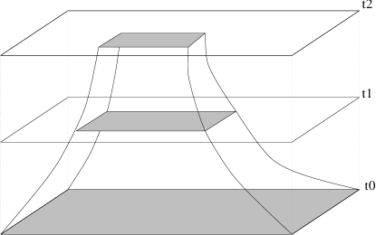
FIG. 1.: Even with an inaccurate, but stable, outer boundary, the region which is causally disconnected from the boundary has finite size after some evolution. We note that in general relativity the coordinate speed of propagation is not one, so it is possible that causal connection to the boundaries does not move at a linear speed, as indicated by the curved edges of the boundary region here.

The boundary condition we use is a simple copying boundary (sometimes called zero order extrapolation). That is, for each point on the physical outer boundary, we copy all the variables from the point nearest the inside. In practice, this condition will prove very effective in several scenarios. It has the effect of canceling the flux difference in the exterior (as the finite differences of the last points will be zero). This is a valid approximation to “outgoing” boundary conditions when the boundary is close to linear perturbation around flat spacetime. In this special case, the sources of the BM system are close to zero and the system approximates a set of linear wave equations, so canceling the exterior flux effectively prevents any incoming information from outside the domain.

Following Ref.[41], we allow octant boundary conditions, which are appropriate for spacetimes with rotational and equatorial plane symmetry. This allows us to simulate black hole spacetimes with symmetries as full 3D problems, while using one eighth the computational resources necessary when evolving on a full grid. Many interesting problems, including Schwarzschild[41], axisymmetric black hole collisions[77] and distorted black holes[24], and even some full 3D data sets with certain dependence on the azimuthal angle[23, 78], can be treated with this symmetry, allowing a great savings in computational resources. Of course, our code can run without this boundary condition also, and as demonstrated through comparisons running full and octant grids [41], the use of octant symmetry does not affect results.

There are many other boundary conditions which are applicable to three-dimensional numerical relativity, which we do not consider here. However, they are worth mentioning. The apparent horizon boundary condition (AHBC)[36, 8] adds a boundary at the causal interior of a black hole spacetime. Recent progress on the outer boundary treatment, such as matching schemes to perturbative[7] or characteristic[79] evolution schemes, look very promising, and could be ultimately used by Cactus. Another promising boundary treatment involves moving the outer boundary to infinity[80] by conformally rescaling the metric, as per Friedrich’s hyperbolic system[49]. This has proven very successful in one-dimensional calculations[81, 82] and higher dimensional calculations with this method should be available soon. Finally, we reiterate that boundary conditions are a major motivation for hyperbolic treatments of the Einstein equations. Through study of the eigenfields and eigenvalues of the transport system they provide more information about the flow of information at the boundaries, which can be exploited in numerical methods[61].

The interior of black holes is usually handled with an isometry condition, which identifies the interior of a black hole with the isometric exterior via inversion through the sphere. This has been crucial in numerous black hole evolutions published to date (see, e.g., [83, 22, 41, 24, 78]. We do not use a three-dimensional isometry condition, as is described in  [41, 20], since we must transform not only the metric and curvature tensor, but also the first order quantities (such as derivatives of the metric and the vector $V_{k}$) which do not transform as a tensor. An isometry could be implemented for the BM formulation in principle, but as we are looking to move to more general methods to treat the black hole, such as an AHBC, we have chosen not to do so at present. Furthermore, as shown in Ref.[41], with certain slicing conditions like maximal slicing, even without AHBC the isometry condition can be ignored and both regions inside and outside the horizon can be evolved, as long as the lapse collapses sufficiently quickly in the vicinity of the singularity. We will make use of this property of maximal slicing in tests presented below. Recent work proposes an alternative to isometry conditions by “stuffing” with matter the interior of black holes[84] (“stuffed black holes”) and we are currently investigating this approach for 3D spacetimes.

C Evolution Schemes

1 The Strang Splitting

Following the numerical discussion of the BM system in Ref. [4], we will split Eq. (1) into two separate processes. The transport part is given by the flux terms

$$\partial_{t}{\bf u}+\partial_{k}F^{k}_{-}{\bf u}=0\;\;.$$ (42)

The source contribution is given by the following system of ordinary differential equations

$$\partial_{t}{\bf u}=S_{-}{\bf u}\;\;.$$ (43)

Numerically, this splitting is performed by a combination of both flux and source operators. Denoting by $E(\Delta t)$ the numerical evolution operator for system (1) in a single timestep, we implement the following combination sequence of subevolution steps:

$$E(\Delta t)=S(\Delta t/2)\;T(\Delta t)\;S(\Delta t/2)$$ (44)

where $T$, $S$ are the numerical evolution operators for systems (42) and (43), respectively. This is known as “Strang splitting” [72]. As long as both operators $T$ and $S$ are second order accurate in $\Delta t$, the overall step of operator $E$ is also second order accurate in time.

This choice of splitting allows easy implementation of different numerical treatments of the principal part of the system without having to worry about the sources of the equations. Additionally, there are numerous computational advantages to this technique, as discussed in [70]. Theoretical and practical advantages for general relativistic hydrodynamics, where the source step couples the equations for the whole system of Einstein plus matter equations, will be detailed elsewhere.

2 The Source update method

Currently, we treat the source integration with a second order predictor-corrector method[72]. During this step, we only need to evolve the 16 quantities which have a source ($g_{ij}$,$K_{ij}$,$V_{k}$ and $\alpha$).

We use standard finite difference notation here. Subscripts denote grid index, and superscripts denote time index. For instance, $u^{n}_{i,j,k}$ is the value of field $u$ at spatial grid point $i,j,k$ and time level $n$. We use the special upper indices $p$ and $c$ to denote the predicted and corrected values during an update cycle, as we define below. In order to update a variable $u$ (running through the 16 quantities with source) at time level $n$ to the future time level $n+1$, we first compute the “predicted value” $u^{p}_{i,j,k}$ at every point $i,j,k$ of our computational grid.

$$u^{p}_{i,j,k}=u^{n}_{i,j,k}+\Delta t\,S(u^{n}_{i,j,k})\;,$$ (45)

where $u^{n}_{i,j,k}$ is $u$ at current time step $n$ and grid point $i,j,k$, and $\Delta t$ is the time discretization interval. With this predicted value of $u^{p}$, we compute the predicted sources and take a corrector step:

$$u^{c}_{i,j,k}=u^{p}_{i,j,k}+\Delta t\,S(u^{p}_{i,j,k})\;.$$ (46)

Finally, the evolved value of $u$ at the next time step $n+1$ is the average of the value at time step $n$ and the correction:

$$u^{n+1}_{i,j,k}=(u^{n}_{i,j,k}+u^{c}_{i,j,k})/2$$ (47)

In practice, the steps (46) and (47) can be combined into one. Note that this is a completely local operation at every grid point, which allows a high degree of optimization[70]. Higher order methods for source integration can be easily implemented, but this will not improve the overall order of accuracy. However, in special cases where the evolution is largely source driven[56], it may be important to use higher order source operators, and this method allows such generalizations.

3 The Flux Update Methods

The implementation of numerical methods for the flux operator is much more involved, and we have many choices at our disposal, ranging from standard choices to advanced shock capturing methods[51, 85, 4]. In this paper, we will limit ourselves to two methods: the MacCormack method, which has proven to be very robust in the computational fluid dynamics field (see, e.g., Ref. [86] and references therein), and a directionally split Lax-Wendroff method. These schemes are fully second order in space and time. Although the Cactus code has a modular structure allowing numerous numerical methods to be plugged in and applied to problems for which they may be best suited, in this paper we restrict ourselves to results with these two methods. Unless otherwise noted, results are generated with the MacCormack method; use of the Lax-Wendroff solver will be explicitly noted.

Following the previous notation we define our fluxes in individual directions $x$, $y$, and $z$ as $FX$, $FY$, and $FZ$ respectively.

The MacCormack method evolves a given quantity $u$, which now runs through the 30 dynamical variables having fluxes ($K_{ij}$,$D_{kij}$,$V_{k}$,$A_{k}$; the $A_{k}$ and $D_{kij}$ only have fluxes in one direction, which is explicitly exploited in our code) with the following algorithm: First, in order to update the variable $u$ to the time level $n+1$, we compute the “predicted value” $u^{p}_{i,j,k}$, with first order backward finite differences:

$$u^{p}_{i,j,k}=u^{n}_{i,j,k} + {\Delta t\over\Delta x}(FX(u^{n}_{i,j,k})-FX(u^{n}_{i-1,j,k}))$$ (48)

$$+ {\Delta t\over\Delta y}(FY(u^{n}_{i,j,k})-FY(u^{n}_{i,j-1,k}))$$ (49)

$$+ {\Delta t\over\Delta z}(FZ(u^{n}_{i,j,k})-FZ(u^{n}_{i,j,k-1}))$$ (50)

where, in addition to the quantities defined above, $\Delta x$, $\Delta y$, and $\Delta z$ are the spatial discretization intervals. Note that this predicted step can be done in a given direction (say $x$), from grid points $2$ to $nx$ (total number of grid points in that direction), as the first order backward differencing only requires $i-1$. With this predicted value of $u^{p}$, we recompute predicted fluxes and sources and take a corrector step with forward finite differencing:

$$u^{c}_{i,j,k}=u^{p}_{i,j,k} + {\Delta t\over\Delta x}(FX(u^{p}_{i+1,j,k})-FX(u^{p}_{i,j,k}))$$ (51)

$$+ {\Delta t\over\Delta y}(FY(u^{p}_{i,j+1,k})-FY(u^{p}_{i,j,k}))$$ (52)

$$+ {\Delta t\over\Delta z}(FZ(u^{p}_{i,j,k+1})-FZ(u^{p}_{i,j,k}))$$ (53)

Now we can correct the interior points of the domain from $2$ to $nx-1$, as we have a prediction for the last plane at $nx$. Finally, the evolved value of $u$ at the next time step $n+1$ is the average of the value at time step n and the correction:

$$u^{n+1}_{i,j,k}=(u^{n}_{i,j,k}+u^{c}_{i,j,k})/2.$$ (54)

A similar method could be obtained interchanging the order or backward and forward derivatives in the predictor and corrector steps. We note that both methods can introduce certain spatial asymmetries in a numerical evolution, due to the preferred order of finite difference operations in the predictor and corrector steps. These asymmetries converge away to second order, as we will discuss below when presenting results.

The directionally split Lax-Wendroff method uses a series of one dimensional Lax-Wendroff integrations to complete a full three dimensional integration step. In one dimension, the Lax-Wendroff scheme is

$$u^{n+1/2}_{i+1/2} = \frac{1}{2}(u^{n}_{i+1}+u^{n}_{i})+\frac{\Delta t}{2\Delta x}(F(u^{n}_{i+1})-F(u^{n}_{i}))$$ (55)

$$u^{n+1}_{i} = u^{n}_{i}+\frac{\Delta t}{\Delta x}(F(u^{n+1/2}_{i+1/2})-F(u^{n+1/2}_{i-1/2})).$$ (56)

Several options exist to turn Lax-Wendroff into a three dimensional scheme. Here we choose directional splitting[72]. Defining $X(\Delta t)$ to be a one dimensional Lax-Wendroff in the $x-$direction, $Y(\Delta t)$ in the $y-$direction and $Z(\Delta t)$ in the $z-$direction we define a full flux time step as $X(\Delta t)Y(\Delta t)Z(\Delta t)$ on the first step, $Y(\Delta t)Z(\Delta t)X(\Delta t)$ on the second step, $Z(\Delta t)X(\Delta t)Y(\Delta t)$ on the third step, and then repeat the prescription. This permutation leads empirically to a second order in space and time scheme, as we shall demonstrate below. The advantage of this directionally split Lax-Wendroff is that, by turning the problem into a set of one dimensional PDEs, implementation of a simple inner (apparent horizon) boundary condition becomes easier, as will be reported elsewhere[87].

D Convergence

Since the pioneering work of Choptuik[88], the usage of convergence tests in numerical relativity is slowly becoming standard practice[41, 7, 9, 45]. The recent discovery and characterization of gauge pathologies[45] stresses the importance of careful convergence analysis, especially in 3D numerical relativity, as simulations may hide solutions that “look” reasonable for a given resolution but do not satisfy the constraints. For completeness, here we review the basis of convergence tests. We will discuss the case of numerical discretization of PDE’s with finite differences. Similar arguments can be developed for other approaches.

Assuming that we have well behaved solutions which allow a expansion in Taylor series, we can relate the numerical solution $\tilde{S}$ to the analytical solution $S$ in the following way:

$$\tilde{S}=S+O(\Delta^{\sigma}),$$ (57)

where $\Delta$ is the grid spacing. Consistent numerical simulations must demonstrate that some form of this relation is obeyed, as the refinement of the grid should always improve the solution. In many cases, it is actually possible to measure the convergence rate $\sigma$. This analysis is crucial if one is to understand how close a given numerical solution is to the true analytic solution, which is generally not known.

Given three discretized solutions, $\tilde{S}(\Delta)$, $\tilde{S}(\Delta/q)$ and $\tilde{S}(\Delta/q^{2})$ we find that

$$L \equiv \tilde{S}(\Delta/q)-\tilde{S}(\Delta)=O\left((\Delta/q)^{\sigma}-\Delta^{\sigma}\right)$$ (58)

$$M \equiv \tilde{S}(\Delta/q^{2})-\tilde{S}(\Delta/q)=O\left((\Delta/q^{2})^{\sigma}-(\Delta/q)^{\sigma}\right).$$ (59)

We define precisely the intuitively clear “-” operator below. Dividing and canceling $\Delta^{\sigma}$ we find

$$\frac{L}{M}=\frac{q^{-\sigma}-1}{q^{-2\sigma}-q^{-\sigma}}=q^{\sigma},$$ (60)

so solving for $\sigma$,

$$\sigma=\frac{\log\left(\frac{L}{M}\right)}{\log q}.$$ (61)

Eq. (61) is the principal definition of the convergence rate $\sigma$ that we will use. In practice, we use $q=2$ for our convergence tests, that is, we double or halve our grid resolution in a sequence of simulations when determining $\sigma$.

The definition of the “-” operator used to form $L$ and $M$ is very important. If the points of $S(\Delta/q)$ and $S(\Delta)$ are coincident on the $\Delta$ grid, then simply pointwise subtraction followed by a norm of the difference can generate the “-” operator. We can schematically represent this operation as

$$\tilde{S}(\Delta/q)-\tilde{S}(\Delta)\equiv|\tilde{S}(\Delta/q)_{qi,qj,qk}-\tilde{S}(\Delta)_{i,j,k}|,$$ (62)

although often more complicated index juggling that simply $i\rightarrow qi$ is required. We note that $|x|$ denotes some norm over the $i,j,k$ space (e.g., maximum, ${\cal L}_{1}$, ${\cal L}_{2}$).

If the points are not coincident, a possibility is to use some norm over the solutions and then define “-” as the difference of those norms. That is

$$\tilde{S}(\Delta/q)-\tilde{S}(\Delta)\equiv|\tilde{S}(\Delta/q)|-|\tilde{S}(\Delta)|.$$ (63)

We call this convergence in the norm. This method has the advantage that it is very easy to calculate during runtime of a parallel code, but is often susceptible to large amounts of noise. If we have an interpolation operator $I^{\Delta/q}_{\Delta}$ which interpolates a solution from a grid with resolution $\Delta/q$ to one with resolution $\Delta$, we can define

$$\tilde{S}(\Delta/q)-\tilde{S}(\Delta)\equiv|I^{\Delta/q}_{\Delta}\tilde{S}(\Delta/q)-\tilde{S}(\Delta)|.$$ (64)

Generally, an interpolator of at least order $\sigma$ is required to do this style of convergence testing.

Finally, when an exact solution is known, we only require two numerical solutions to the equations to measure $\sigma$. That is, given a discretized solution at $\tilde{S}(\Delta)$ and $\tilde{S}(\Delta/q)$ and an exact solution $S$, we can form two differences pointwise,

$$L = S-\tilde{S}(\Delta)={\cal O}(\Delta^{\sigma})$$ (65)

$$M = S-\tilde{S}(\Delta/q)={\cal O}(q^{-\sigma}\Delta^{\sigma})$$ (66)

and therefore find the relationship

$$L=q^{\sigma}M,$$ (67)

and again we recover $\sigma$ from Eq. (61). Simply said, for a second order method, the error should be four times larger on the coarser grid than the finer grid. This method will prove valuable for calculating convergence against known solutions, convergence of constraints, and convergence of fictitious numerical errors, such as asymmetries.

As before, we are faced with the problem of computing the quotient $L/M$ accurately, especially in the case of fields which go to zero. Once again, we can solve this problem by interpolating $M$ onto the grid which $L$ inhabits and forming the quotient pointwise.

When the convergence rate is expected to be second order, with this technique we can also measure $\sigma$ graphically at all points. That is, if we have a known solution $S$, we can plot, $\tilde{S}(\Delta)-S$, $(\tilde{S}(2\Delta)-S)/4$, $(\tilde{S}(4\Delta)-S)/16$ and so forth. If the points agree, then we have second order convergence. This method has the advantage that point to point noise present in calculating $\sigma$ can be eliminated “by eye,” and we shall use this method often below.

Convergence testing is an essential component of a battery of code tests. Demonstrating that an evolution scheme has the appropriate convergence order shows that boundary treatments, methods, and infrastructure are coded properly. Studying convergence properties can help diagnose and track subtle errors in a code. However, showing that, for example the metric function $g_{xx}$ converges does not imply that one is solving the Einstein equations; it merely means that one is solving the coded evolution equation to second order. Thus, convergence testing against known solutions is important. In a few rare cases, notably a geodesically sliced black hole, there are exact solutions to the non-linear dynamical Einstein equations. In this case one can show not only that numerical results converge to something (that is, we find $\sigma=2$ using definitions (61)), but also that they converge to the right thing (that is, we get order $\sigma=2$ when comparing against the known solution, using the definition (67)).

With the Einstein equations, however, we play on favorable ground, as we always have an analytic solution at our disposal: the vanishing of the constraints. That is, all correct solutions to the fully nonlinear Einstein equations have the property that the hamiltonian and momentum constraints must identically vanish. Regardless of the relativistic system being simulated, if the initial data satisfies the constraints, then so must all subsequent time steps. We assume the behavior of the hamiltonian constraint, $H$, is

$$H(\Delta x)=0+E(\Delta^{\sigma}),$$ (68)

where $E(\Delta^{\sigma})$ is the error due to finite differencing with a spatial step $\Delta$. Choptuik has investigated this point at great length in Ref.[88], where he shows that for a consistent finite differencing of the free evolution of the Einstein equations, the constraints have the same order error as the evolution scheme. Choptuik demonstrated this in spherical symmetry, and here we demonstrate this in full three dimensional numerical relativity. With relation Eq. (68) in hand, forming $L$ and $M$ in the language of Eq. (66) simply amounts to looking at the value of the constraint. If we double the resolution, and the numerical code is solving the Einstein equations, our constraints must drop by a factor of four (for a second order scheme) everywhere. (We note that one may use the constraints to eliminate one of the evolution equations, and with this approach it would be reasonable to expect that the code could demonstrate an independent construction of the eliminated evolution equation converging to zero, rather than the constraint.)

Having discussed the convergence techniques we use to study the performance of the Cactus code, we describe briefly our philosophy of their use before moving on to examples below. An important point is that a 3D code should exhibit convergence, even if the resolution is too low to exhibit a high degree of accuracy. For instance, a given numerical result may differ from the true analytic solution by a large factor. This is not necessarily a major concern, as long as doubling the resolution can quarter the error. By running simulations at different resolutions, one can then estimate how close the numerical solution is to the analytic solution, understand the behavior of the truncation error, and estimate the resolution required to obtain a solution to the desired accuracy. We regard this as a crucial requisite of a code, which as we show below, our code has.

We note that it is possible that resolution can be too low to allow an evolution beyond a certain point. For instance, a geodesically sliced black hole with very low resolution may crash before (or after) a higher resolution simulation, since there is a physical singularity present. However, in this case convergence should show the region in which the simulation is accurate. When a solution starts failing to converge, the evolution is probably about to fail. We will see an example of this in Sec. VI C. Convergence at the boundaries also offers useful information. Using our simple “copying” boundary condition without any advanced treatment of the system, we expect that condition to have a first order effect on phenomena which interact with the boundary. Finally, we regard second order convergence to be desirable, but not necessary, in order to verify a given numerical result. For instance, often one does not have second order convergence near boundaries. But such an effect can be studied and understood. The key point is that one should know that a code converges at or above the expected order, even if that order is one.

IV Flat Space Tests

A Dynamically sliced Flat space

One of the crudest first tests of any 3D cartesian based code is, given geodesically sliced Minkowski space, does the code produce 1 and 0 forever. Of course Cactus does, but this test is almost useless, since one cannot measure convergence, and all constraints are trivially satisfied. A more interesting and much more important test is that of a dynamically sliced flat spacetime. That is, we choose an initial lapse in Minkowski space which is not unity everywhere, and then we evolve this system with a “live” slicing condition on the lapse $\alpha$, such as harmonic slicing. Such an idea has been suggested in the past by York [48] and also implemented and studied in detail by Massó[56]. We have examined three distinct cases, 1D periodic data (e.g., $\alpha$ is a periodic function of one coordinate only), 3D periodic data, and 3D data where $\alpha$ falls off to unity at large radii. The first two allow us to study Cactus without boundary affects, and the last allows us to evaluate the quality of our boundary conditions. In this section we present 3D simulations with “copying” boundary conditions and harmonic slicing, and in the following sections we also chose various shifts in both one and three dimensions. Simulations here are performed with the Einstein system ($n=1$).

We note this problem is similar to the example used to study coordinate conditions discussed in [43], but with some important differences. First, we evolve with harmonic slicing throughout the entire evolution, rather than using the lapse to generate a small “bump” in tr$K$, followed by maximal slicing, as in Ref. [43]. Secondly, in harmonic slicing of flat space, the lapse evolution equation becomes wavelike, so our initial pulse travels off the grid as a wave pulse.

In the 3D case, we choose an initial lapse with a gaussian bump specified by

$$\alpha=1+A\exp\left(\frac{r^{2}}{\sigma^{2}}\right).$$ (69)

In the 1D case, we choose an identical form, simply replacing $r$ with $x$, $y$, or $z$. In both cases, we see simple wave-like propagation in the lapse, as demonstrated below. For our first test, we evolve this dynamically sliced flat space system in 3D with a resolution $\Delta x=\Delta y=\Delta z=0.01$ on a grid of $101^{3}$ centered around $r=0$. We choose the parameters $A=0.05$ and $\sigma^{2}=0.05$. Two-dimensional slices in the $z-$plane of the evolution of this initial lapse in a harmonically sliced spacetime, with “copying” boundary conditions discussed in Sec. III B above, are shown in Fig. 2. Other metric functions, although initially taking a Minkowskian form, develop similar dynamics.

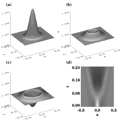
FIG. 2.: We show slices of the evolution of the lapse in the 3D dynamically sliced flat spacetime described in the text. Figures (a), (b), and (c) show slices in the $z=0$ plane at times $t=0.0$, $0.1$, and $0.2$. In Figure (d) we show the value of $\alpha$ on the $y=0$, $z=0$ line evolving in time as a colored contour map. We note that in this simulation, the majority of the pulse has not yet hit the boundary of the computational domain. $101^{3}$ grid points were used with a resolution of $\Delta x=0.01$.

We demonstrate that the hamiltonian constraint converges at second order in the interior in Fig. 3, where we show the constraint at three different resolutions, with the appropriate factors of four and sixteen. The fact that the lines are coincident demonstrates second order convergence. The actual value of the convergence exponent on the grid is above 1.9 for the entire evolution, until the pulse interacts strongly with the boundary.

FIG. 3.: We demonstrate convergence of the hamiltonian constraint to zero in the interior of the 3D evolved dynamically sliced flat space. Although the $x-$axis is shown here, other directions have similar results. The fact that the high resolution hamiltonian is equal to one-quarter the medium resolution, and this one is itself one-quarter the lower resolution, indicates that the hamiltonian converges rigorously to zero at second order in the interior. However, the logarithmic scale reveals, at a very low level, a lack of second order convergence near the boundaries at later times. This is caused by our outer boundary condition, which is not expected to be second order accurate.

We noted above that due to the upwind/downwind nature of the MacCormack predictor-corrector method we use, certain asymmetries in the evolution are introduced. In Fig. 3 we see that symmetry around the origin of the coordinate system is not maintained except in the limit of a converged solution. (We note rotational symmetries are obeyed. By this we mean that, given symmetric data, our code will generate identical solutions along an $x$-directed and $y$-directed slice of our data. However both of these solutions will be (identically) asymmetric around the origin.) This asymmetry is purely an artifact of our method having an upwind/downwind nature, as shown in the finite difference representation. As such, this asymmetry should converge away at second order. In Fig. 4 we show that this asymmetry is an artifact of numerical error, and consequently, converges to zero by measuring the asymmetry, $E=\alpha(x)-\alpha(-x)$, for the evolved flat space case. Clearly this should be zero in the converged limit, so the numerical solution should obey $E(\Delta x/2)=E(\Delta x)/4$ if our method converges at second order. From Fig. 4 we see that this relationship is obeyed except at the boundaries, where our boundary condition imposes a first order asymmetry on the system at late times.

FIG. 4.: We show symmetry violation due to the MacCormack predictor corrector method, and how that converges away. For the dynamically sliced flat space model, we show $E=\alpha(x)-\alpha(-x)$ for $x>0$ at the times $t=0.8$, $t=0.16$ and $t=0.24$. We show $E/4$ at a low resolution (dotted line) and $E$ at twice the resolution (solid line). The fact that the high resolution error is less than or equal one-quarter the low resolution error indicates that the method’s asymmetry converges to zero at second order. An interesting feature of this figure is that it demonstrates the first order nature of our boundary condition clearly. Since the lapse becomes dynamic on the boundary at later times, convergence order drops from two (which the evolution system obeys) to one (which the boundary condition obeys) as the wave propagates towards and through the boundary.

Figs. 3 and 4 also give an interesting indication of our boundary conditions when dynamics are present at the boundaries. As shown in Fig. 2, the traveling pulse in the lapse is approaching the boundary by late times in our simulation. Once the dynamics reach the boundary, convergence drops from second order towards first order there. This is indicated in Fig. 4 by the high resolution case (solid) having more than one-quarter the error of the low resolution case (dotted line), and by non-second-order convergent (although small) errors in the hamiltonian constraint, as shown in Fig. 3. That is, the solid line is above the dotted line.

So far, we have only measured convergence of metric functions and constraints. We can also examine the physical properties of our underlying spacetime. In this spacetime, we can demonstrate that we are evolving Minkowski space by measuring the Riemann invariants $I$ and $J$, computed using a $3+1$ method[89]. These should be identically zero, but they will not be due to finite differencing errors. However, we can test how they behave with varying resolution. In Fig. 5 we show $|I|$ at three different resolutions for the distorted flat space case considered here. We note that, firstly, $|I|$ is small, and also that it decreases faster than second order with grid resolution towards zero. In fact, in this case the convergence exponent for $|I|$ is very close to four. Clearly boundary effects are evident, driving the system away from the underlying flat space.

FIG. 5.: We show the Riemann invariant $|I|$ along the $x$-line in the dynamical flat spacetime at various resolutions. We show the invariant at three resolutions with appropriate factors of $1/4$ and $1/16$, and note that the invariant is converging towards zero faster than second order. In this case, the convergence exponent is very close to four.

B Testing the Shift

We now introduce the shift vector $\beta^{i}$ to test its effect on the solution. The dynamically sliced flat spacetime is an excellent case to test the shift terms in Cactus. We first examine a constant shift, and then move to a spatially varying shift to test all terms related to the shift vector.

1 A Test of a Constant Shift

As a first simple test, we chose the one dimensional periodic initial lapse, and evolve this on an explicitly 1D grid with periodic boundary conditions (that is, we use Cactus on a $(nx,1,1)$, $(1,ny,1)$ or $(1,1,nz)$ sized grid). The initial lapse is chosen the same as in Eq. (69), with $r$ replaced with $x$, $y$, or $z$ alone, with $\sigma^{2}=0.05$. In this harmonically sliced system with a constant shift, the evolution equations become wavelike for the lapse, with the propagation velocity being $1\pm\beta$.

In Fig. 6 we see exactly this propagative behavior. The lapse function $\alpha$ is shown for three cases, $\beta=0$ and $\beta\pm 1$. For $\beta=0$, the wave propagates with speed $c=1$ in both directions. For the shift chosen as $\pm 1$ we see the speed of the waves to be two or zero, depending on the direction of propagation and the sign of the shift. This can be clearly read from the graph, where the propagation in the $t$ direction (vertically) is $0.5$ in all cases, and the propagation distance in the $z$ direction is $0.5$ in the zero shift case, and $1.0$ and $0.0$ in the $\pm 1$ shift case. The other metric functions, not shown, exhibit similar behavior.

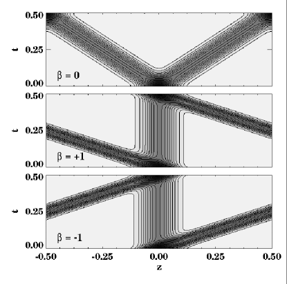
FIG. 6.: We show propagation of the lapse in a dynamically (harmonically) sliced Minkowski space where the initial lapse is chosen to be a periodic gaussian function of $z$ alone. We see the expected affect of the shift. That is, shifts of $\pm 1$ force the propagation of the lapse to have zero coordinate speed in one direction.

2 A Test of a Spatially Dependent Shift and an Important Lesson

We next turn to a spatially non constant shift as a test of our code,

$$\beta^{x}=\beta^{y}=\beta^{z}=Ae^{-(x^{2}+y^{x}+z^{2})/{\sigma}^{2}}.$$ (70)

We here only consider the cases of $A<1$, a sub-tachyonic shift. The gaussian width $s$ is chosen so the shift is resolved but effectively vanishes before the boundaries. This choice of shift will test all terms in our (non-conformal) evolution equations, since it has derivatives of all shift terms in all directions. The following runs were performed with $\Delta x=\Delta y=\Delta z=0.01$, $\sigma^{2}=0.02$, $A=0.5$, and with $101$ grid zones in each direction.

Using this shift, we discovered an error in our code, which is worth discussing. In an initial version of our code, we had an error in the shift term for the sources of the $V$ variables. Rather than the correct term,

$$2({D_{ri}}^{s}-\delta_{i}^{s}{D^{j}}_{jr}){B^{r}}_{s}$$ (71)

we had the different, although very similar,

$$2({D_{ri}}^{s}-\delta_{i}^{s}{D^{j}}_{jr}){B_{s}}^{r}.$$ (72)

(Recall that $B$ is not symmetric.) As we show now, by only performing convergence tests we were able to diagnose and track down the code error, without appealing to any analytic solutions beyond the vanishing of the constraints.

In Fig. 7 we show the evolution after some time choosing the shift in Eq. (70), with and without the error above. As is clear, the evolutions are very similar; in fact, had two different codes given this result, without further testing one would be tempted to say the results are the “same” and so the codes “agree”.

FIG. 7.: We show two evolutions of $\alpha$ in our distorted flat space model with a spatially dependent shift, using the Einstein equations in one case, and the equations with a small error in the second. In (a) we show the numerical solution after eight iterations for the case with the correct shift terms with a solid line, and the results with an error in the shift with a dashed line. At this level, the plots are indistinguishable. In (b) we show the difference between the two evolutions, and notice the difference is negligible compared to the disturbance in the lapse.

However, in Fig. 8 we show that the hamiltonian constraint, as defined by Eq. (35), converges to zero for the Einstein equations, and fails to do so for the system which is not. The failure to converge is clear and large. We note that even with fairly low resolution we can demonstrate that our code is correct or incorrect by showing merely the convergence of the constraints and we did not need an exact solution for the spacetime (other than the vanishing of the constraints). We feel that this clearly demonstrates that convergence testing constraints is an important and strong test of any code.

FIG. 8.: We show the convergence of the hamiltonian constraint for the Einstein equations above and the non-convergence of the constraint for the Einstein equations with an error below. We note that even though the error in our lapse evolution is very small, the convergence simply fails for the incorrect equation (note in the lower plot that the hamiltonian is the same for both resolutions, although the figure might mislead the reader because we introduce the factor of 4 that we would expect for convergent results). Again, this demonstrates second order convergence for the correct equations. We note that in both cases the hamiltonian constraint is “large”; about 0.2 in the high resolution correct case (0.8 in the low resolution case) and about 15 in the incorrect case (being non convergent, stays the same for both grid resolutions). The only way to determine if the constraint is too “large” is to test its convergence towards zero, which is a feature of only the Einstein equations in this case.

V Wave Spacetime Tests

Although hyperbolic reformulations of the 3D Einstein equations have not been used in a wide variety of spacetimes before this publication, they have been applied to linearized wave spacetimes[41, 7]. The current version of this code owes much to the implementation of the “H” code described in Ref.[90]. As we reviewed in the introduction, this “H” code used a previous BM formulation of the equations that required the exclusive use of harmonic slicing and zero shift vector [2]. That code is now obsolete, although all the tests of the “H” code described in Ref. [41] can be replicated successfully by this new and much more advanced version of the code. All the tests presented here are run with the “Ricci” system ($n=0$), as this corresponds more closely to the simulations performed with the “H” code. Here we detail some of these comparisons, evolving linear initial data that describe weak gravitational waves. The interesting transition from linear to non-linear effects described in Ref. [42] will not be studied here, although it is possible to reproduce those effects with the two formulations (BM and ADM) implemented in Cactus.

Further studies of stronger gravitational wave interactions and their possible collapse to a black hole are underway and will be described in a future publication in this series, where appropriate slicing conditions for wave spacetimes will be considered in detail. In this section, we will focus on two cases, colliding plane waves and quadrupolar waves, and limit our gauge to harmonic slicing.

A Plane Waves

We consider linearized plane wave solutions, following the test in section III of Ref. [41]. The line element is written

$$ds^{2}=-dt^{2}+(1+f(t,z))dx^{2}+(1-f(t,z))dy^{2}+dz^{2}.$$ (73)

For small $f$, the linearized Hamiltonian constraint is satisfied, and the evolution of the spacetime is governed by the linear wave equation

$$\partial_{t}^{2}f(t,z)=\partial_{z}^{2}f(t,z),$$ (74)

that describes plane waves propagating in the $z$ direction. We use the Gaussian-shaped packet:

$$f(t,z) = A_{R}e^{-(2\pi(t-z-a)/\sigma)^{2}}\cos\left(\frac{2\pi}{\lambda}(z-t)\right)$$ (76)

$$+A_{L}e^{-(2\pi(t+z-a)/\sigma)^{2}}\cos\left(\frac{2\pi}{\lambda}(z+t)\right)\;,$$

The amplitudes $A_{R}$ and $A_{L}$ represent the amplitudes of waves traveling to the right and left, respectively, with a Gaussian shape of width $\sigma$ and centered at $z=\pm a$ at $t=0$. $\lambda$ is the wavelength of the Gaussian-modulated oscillations.

In Fig. 9 we show the evolution of the metric component $g_{xx}$ for a single wave moving in the $-z$ direction. We have chosen the shape parameters $\sigma=2$,$\lambda=1$,$A_{L}=0.00001$, $A_{R}=0$ and $a=3$, with $\Delta z=0.025$. This figure replicates Fig.1(a) of Ref. [41], which used an ADM code with an staggered-leapfrog algorithm. We notice that the wave is transported with a small loss of amplitude, due to dispersive effects in the MacCormack predictor corrector scheme. The measured convergence $\sigma$ is very close to 2. This is one of the simplest tests of a numerical code designed to evolve waves and the results obtained are in agreement with the well-known numerical properties of our standard methods applied to the linear wave equation.

FIG. 9.: We show the evolution of $g_{xx}$ for a single plane wave moving in the $-z$ direction at times $t=0$, $t=3$ and $t=6$ for a gaussian wave packet. This figure replicates Fig. 1(a) of Ref. [41]. The dispersive nature of the MacCormack method can be appreciated in the non-symmetric propagation of the gaussian packet.

A more involved test results from colliding plane waves. Unlike the previous test, in this case we deal with nontrivial spacetimes: theoretically, it is known that such spacetimes will develop a singularity in the future (in the non-linear regime) [91, 92]; numerically, coupled nonlinear and finite differencing effects can lead to spurious numerical evolution [41]. Hence, they provide a stronger test of a numerical code. In Fig. 10 we show the evolution of a colliding wave system. Two wave packets originally start, moving inwards, centered at $z=\pm 3$. We choose the same parameters as the single wave packet except for the amplitudes $A_{R}=A_{L}=0.025$. The packets collide at the center at time $t=3$ and then continue on. Once again, dispersion is visible when the waves return to their original images at $t=6$. This figure replicates Fig. 6(d) of Ref.[41]. There it was shown that the staggered-leapfrog method was prone to a large secular drifting after the packets collided, which does not occur with our MacCormack method.

FIG. 10.: We show the evolution of $g_{xx}$ for two colliding plane wave packets. At $t=0$ the two packets are centered at $z=\pm 3$, they collide and superimpose at $t=3$. At $t=6$ the left and right packets have interchanged their positions and should be coincident with their shapes at the initial time. The difference is due to numerical dispersion. Continuing the evolution, the packets are more dispersed at $t=9$. This figure replicates Fig. 6(d) of Ref. [41]. The MacCormack method used here does not exhibit the drifting after the collision exhibited by the staggered-leapfrog method in Fig. 6(a) of that reference.

B Pure Quadrupolar waves

The numerical simulation of quadrupolar linearized wave solutions to the Einstein equations has been established as an standard test of 3D numerical codes[7, 41, 93]. One of the reasons of their appeal is the existence of a family of analytic solutions for both even- and odd-parity and the independent azimuthal modes[94]. But more importantly, we also need to model their evolution accurately, as quadrupolar modes are a dominant signal in the late time evolution of black hole spacetimes. In this section we compare evolutions of quadrupolar waves in Cactus with previous results, following again the extensive tests and discussions of Ref.[41]. Due to the length of the analytical expressions, we do not write the solutions here and refer to the reader to Ref.[94] or Ref.[95].

We start by evolving even-parity waves with an amplitude of $10^{-5}$ and quadrupole numbers $l=2$ and $m=0$. The details of this setup are given in section VI of Ref.[41]. In Fig. 11 we show the evolution of $g_{xx}$ along the $z$–axis performed on a grid of $120^{3}$ points with $\Delta x=\Delta y=\Delta z=0.05$. This replicates Fig. 9(c) of Ref.[41]. We can see how an initially moderate wave packet near the center of the grid oscillates and propagates off the grid, as expected.

FIG. 11.: The evolution of metric function $g_{xx}$ along the z line is shown for linear quadrupolar waves with $l=2$, $m=0$ and a low amplitude packet, which corresponds to a perturbation of 0.025% in the metric functions. The wave expands outward as time increases, returning to a flat profile after $t=4$. This replicates Fig.9(c) of Ref. [41].

FIG. 12.: We show the time evolution of the wave-like quantity $r(g_{xx}-1)$ measured at the outer boundary for the simulation shown in the previous figure. The wave pulse arrives to the boundary at around $t=4$, oscillates and leaves the computational grid. This serves as indicator of the outgoing condition provided by our simple copying boundaries

In Fig. 12 we show the time evolution of the quantity $r(g_{xx}-1)$ at the outer boundary of our grid, as an indicator of the clean outgoing condition provided by our simple copying boundaries. This measure of the wave simply separates the perturbation from the background Minkowski metric, and corrects for the $1/r$ falloff. It is not a gauge-invariant measure of waves, such as that used in Ref. [78]. Detailed studies extending these results beyond linear wave regimes are under way and will be published elsewhere.

Ironically, the extensive work of Ref.[41] does not include results with any truly 3D spacetime, as the cases studied for quadrupolar waves correspond to axisymmetric waves of azimuthal number $m=0$. In this paper we will extend the results of that reference by setting up a slightly more realistic scenario, tuning the parameters to mimic what we expect from late time ringdown of black hole simulations. Therefore, we will evolve non-axisymmetric quadrupolar waves with $l=2$, $m=2$ and a stronger amplitude wave, with $A=0.001$, corresponding to a perturbation of 3% in the metric components. In this full 3D case, we do not use an octant of the spacetime, but rather set up a full grid with the origin in the center. Again, the grid has $120^{3}$ points with $\Delta x=\Delta y=\Delta z=0.05$. As we have a full grid, the outer boundary is now closer. In Fig. 13 we see the evolution of the now stronger initial packet propagate outwards, as expected. In Fig. 14, we again show the “waveform” measured directly by the function $r(g_{xx}-1)$ at the outer boundary, which is allowing the wave to cleanly propagate off the grid. At late times boundary effects become visible. See Ref.[7] for an excellent discussion of the problem of outgoing conditions in this scenario and possible solutions with perturbative techniques.

FIG. 13.: We show the evolution of $g_{xx}$ for the $l=2$, $m=2$ stronger amplitude quadrupolar wave packet along the $z$–axis. The perturbation on the metric components is around 2.5% for this higher amplitude. Although this packet is fully 3D and can not be evolved using an octant of the spacetime, the metric component $g_{xx}$ is symmetric around the origin.

FIG. 14.: We again show the time evolution of $r(g_{xx}-1)$ at the outer boundary for the simulation shown in the previous figure. Again, although our simple copying boundary condition, coupled with the MacCormack method, does a reasonably good job of allowing the wave to propagate through the boundary, at late times boundary effects are evident. Note that the outer boundary, at $z=\pm 3$, is now closer to the origin.

To better visualize the temporal evolution of this wave, in Fig. 15 we show the value of $r(g_{xx}-1)$ along the $z-$axis evolving in time as a surface. We can see that the wave propagates cleanly away from the center and off the boundaries, as expected.

FIG. 15.: We show the time evolution of the “extraction” function $r(g_{xx}-1)$ along the $x$ line. The surface plot has time along the $y$–axis. The $r$ factor corrects for the $1/r$ fall-off, so we can see that the wave propagates from the center and off the boundaries. The previous figure corresponds to the $y$–axis (i.e., time) boundary of this plot.

The best way to visualize the full 3D nature of these waves and their propagation would be to show a movie, which obviously we can not do in printed form. In Fig. 16 we show four snapshots of such a movie, showing two isosurface values of the metric component $g_{rr}$, constructed from the cartesian metric.

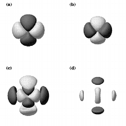
FIG. 16.: We show four time snapshots of the evolution of the packet presented in the last figures. Two isosurface values of the spherical metric component $g_{rr}$, reconstructed from the evolved cartesian components, are shown at times $t=0$ (a), $t=1$ (b), $t=2$ (c) and $t=3$ (d). The dark and light colored isosurfaces correspond to the values $0.9997$ and $1.0003$ respectively. They oscillate around the center and propagate outwards.

All the wave tests presented in this section converge as expected. In Fig. 17 we show the time evolution of the convergence rate $\sigma$ obtained using the ${\cal L}_{2}$ (i.e., RMS) norm over the entire grid. We measure convergence for the hamiltonian constraint, the metric component $g_{xx}$, and the lapse, and note that all converge at or above second order, as expected. We do not need to resort to the linear solution to measure convergence. In this special case, we do not measure the convergence of the constraints to zero, as the initial data is linear and only satisfies the constraints to linear order. Thus, we measure the convergence of the hamiltonian as we would any other quantity, using three different resolutions to create the convergence exponent.

FIG. 17.: We show the time evolution of the global convergence rate (computed in the ${\cal L}_{2}$ norm) of the hamiltonian constraint, $g_{xx}$ and the lapse function. All quantities converge at second order. In particular, the hamiltonian constraint converges also at second order, although it does not converge to zero, since it is only satisfied to linear order.

VI Black Hole Tests

Black hole spacetimes are currently one of the major motivations for developing 3D numerical relativity. The waveforms emitted by inspiraling colliding black holes are expected to be one of the most likely candidates for early detection by laser interferometers[6, 5], and hence are urgently in need of general 3D simulations. Thus, black hole spacetimes are important tests of our code, and we will follow the work of Ref. [19] in these code tests of Schwarzschild black holes. More dynamic black hole studies, including the simulations of 3D excitation and ringdown of the quasinormal modes of distorted black holes [25, 78, 24, 96], and of black hole collisions [18], are in progress and will reported and compared against published results in a future paper in this series.

Black hole spacetimes are in many ways similar to other spacetimes. An initial metric evolves with some slicing conditions, and the constraints should converge as in any spacetime. However, special difficulties are encountered due to the presence of singularities. Thus, as discussed in the introduction, present Cauchy evolutions of general 3D black hole spacetimes do not allow a 3D code to run forever, as they can when propagating disturbances in flat space or low amplitude waves. At some point, a time slice may hit a singularity and crash, or stretch the grid so much that the simulation will no longer be able to continue. At this point, we will see “blow ups” on our grid, convergence will fail (starting, usually, at the lower resolution grids), and we will have to stop our code. Thus evolving black holes for many tens of $M$, where $M$ is the ADM mass, with a demonstration of convergence is still “state of the art” in numerical relativity.

In this section, we test Cactus using a single black hole with the Einstein-Rosen bridge topology with an isotropic radial coordinate $r$. That is, the spatial line element takes the form

$$ds^{2}=\Psi^{4}(dr^{2}+r^{2}d\Omega^{2})$$ (77)

with

$$\Psi=1+\frac{M}{2r}.$$ (78)

We satisfy the constraint equations with this metric and initial $K_{ij}=0$. For more detail, see Ref. [19]. For all the work which follows, we choose $M=1$.

This data is isometric in inversion through the sphere, or throat, located at $r=\frac{M}{2}$. The singularity at $r=0$ is also related to the remapping of a second universe on the other side of the bridge to the origin in our flat space. However, rather than evolve the Einstein-Rosen bridge black hole spacetime with the natural $S^{2}\times R$ topology (as used in axisymmetric simulations such as [97, 98]), we evolve it on an $R^{3}$ manifold which contains a point where the conformal factor is infinite. This was one of the techniques used in Ref. [19], and has recently been generalized to generate full 3D, binary black hole data with spin and momenta[99].

As in Ref.[19, 20], we handle the infinity in the conformal factor numerically using two tricks. First, we do not place a grid point at $r=0$, but rather we stagger the origin, with grid points at $\Delta x/2$ and $-\Delta x/2$. Secondly, we exploit knowledge of the conformal factor and its derivatives in our finite differencing. This allows us to factor out the infinity from the evolved quantities as known derivatives in the source terms, and evolve fields which are unity everywhere. This approach to computing “conformal derivatives” is quite general, and can be used with a numerically generated initial data set as well. Note that this conformal rescaling of the equations, as discussed in Sec. II D and Appendix A. is different from the conformal rescaling done in typical ADM codes, including the Cactus ADM thorn, where the Ricci tensor is formed directly with conformal derivatives of the system. For our first order system, we do not form the Ricci tensor, and therefore we must treat the conformal rescaling differently in order to preserve a first order system, and still allow only conformal variables to appear in the fluxes.

Here we consider various slicings of a single black hole spacetime. We do not discuss or demonstrate multiple black hole or distorted black hole spacetimes here, since we wish only to show code tests at this time. However, preliminary tests show that the results presented here carry over into more dynamical black hole spacetimes. This is a major and active research area in 3D numerical relativity in which we are presently engaged. In the final part of this section, we also perform tests of the Schwarzschild black hole system with the ADM equations in Cactus, and compare with the results from the BM formulation. All simulations in this section are done with $\Delta x=\Delta y=\Delta z$, $nx=ny=nz$, and with the conformal rescaling of the BM system, or conformal differencing in the ADM system. For the BM system, all simulations were performed with the Einstein system.

A Geodesic Slicing

A black hole spacetime evolved with geodesic slicing ($\alpha=1$, $\beta^{i}=0$) can only be evolved until points initially on the throat hit the singularity unless points are excised from the grid, as shown in Refs. [19, 20]. At that point any code evolving this system will crash. We know that observers initially at rest in the Schwarzschild spacetime that this crash must come at $t=\pi M$. The crash will appear as an infinity or undefined value at a point on the numerical grid.

Despite this critical failing, the geodesically sliced Schwarzschild spacetime is useful as an analytic solution for the three-metric exists, the Novikov solution [100]. This solution expresses the metric in terms of cyclic infall times for initially non-moving observers. Expressions for these solutions in isotropic radius are given in [20], although the final term is missing a square root, thus for completeness we give expressions here [101]. We use a slightly different notation than Ref. [20]: $r$ is our isotropic radius, $r_{\rm{a}}$ is the areal radius, $r_{\rm{max}}$ is the maximum (areal) radius for an observer during the cyclic infall (and is therefore the initial areal radius, so $r_{\rm{a}}=r_{\rm{max}}$ at $\tau=0$), $\tau$ is the proper time of an observer (and therefore the coordinate grid time, as $\alpha=1$), and $g_{rr}$ and $g_{\theta\theta}$ are the conformal isotropic metric components. The relevant expressions for an $M=1$ black hole are

$$r_{\rm{max}}(r) = \frac{(1+2r)^{2}}{4r},$$ (80)

$$\tau(r_{\rm{a}},r_{\rm{max}}) = r_{\max}\left(\frac{r_{\rm{a}}}{2}\left(1-\frac{r_{\rm{a}}}{r_{\rm{max}}}\right)\right)^{\frac{1}{2}}$$ (82)

$$+2\left(\frac{r_{\rm{max}}}{2}\right)^{\frac{3}{2}}\rm{arccos}\left(\left(\frac{r_{\rm{a}}}{r_{\rm{max}}}\right)^{\frac{1}{2}}\right),$$

$$\frac{\partial r_{\rm{a}}}{\partial r_{\rm{max}}} = \frac{3}{2}-\frac{r_{\rm{a}}}{2r_{\rm{max}}}$$ (84)

$$+\frac{3}{2}\left(\frac{r_{\rm{max}}}{r_{\rm{a}}}-1\right)^{\frac{1}{2}}\rm{arccos}\left(\left(\frac{r_{\rm{a}}}{r_{\rm{max}}}\right)^{\frac{1}{2}}\right),$$

$$g_{rr} = \left(\frac{\partial r_{\rm{a}}}{\partial r_{\rm{max}}}\right)^{2},$$ (85)

and (86)

$$g_{\theta\theta} = \left(\frac{r_{\rm{a}}}{r_{\rm{max}}}\right)^{2}.$$ (87)

To construct the metric, we must numerically invert relation Eq. (82) to find $r(\tau,r_{\rm{max}})$. Simple bisection solves this problem. Aside from this minor complication, constructing the solution is straightforward.

We present here two demonstrations that our code is in fact creating the correct solution for the geodesically sliced black hole spacetime. In Fig. 18 we show the difference between the $g_{rr}$ produced by the code (which is constructed from the full evolved cartesian three metric) and the analytic expression in Eq. (VI A). We extract the data along a diagonal line. We show the difference at three different resolutions, adjusting the lower resolution differences by factors of 1/4 and 1/16, respectively. We note that the points (shown as crosses, diamonds, and triangles) are, for all practical purposes, identical in this figure, strongly indicating second order convergence at every point on the grid.

FIG. 18.: We show the difference of the radial metric between the analytic Novikov solution and the full three-dimensional numerical evolution. Data is extracted along a diagonal line. We define $E$ as the difference between the analytic solution and the numerical solution. We show $E/16$ for $\Delta x=0.2$, $E/4$ for $\Delta x=0.1$ and $E$ for $\Delta x=0.05$. We note that the data points are practically identical, showing second order convergence.

In Fig. 19, we show similar plots for the hamiltonian constraint. We show the lower resolution constraints divided by 4 and 16 respectively. Once again, the fact that these lines are visually coincident (although not completely identical) strongly demonstrates that our code is converging at second order. Note that the error is largest near the throat, located at $r=0.5M$, which is well inside the horizon at late times as it rushes towards the singularity.

FIG. 19.: We show the hamiltonian constraint, $H$, for the geodesically sliced black hole at three different resolutions. We show $H/16$ for $\Delta x=0.2$, $H/4$ for $\Delta x=0.1$ and $H$ for $\Delta x=0.05$. We note that the lines are identical, indicating second order convergence.

From these two diagrams we can calculate four values of the convergence exponent everywhere, since we have two quantities to measure against exact solutions, at three resolutions. Doing this analysis gives a convergence exponent between about 1.8 and 2.1 (oscillatory in time), once again demonstrating second order convergence to an exact solution.

The black hole spacetime also provides a strong test of a code’s ability to preserve the appropriate spherical and rotational symmetries inherent in the initial data set. Especially near the singularity, there is a rapid growth of strong gradients surrounding a black hole, which must be computed in the separate cartesian metric functions on a cartesian grid. These individual functions do not exhibit the underlying symmetries of the black hole, so it can be difficult to model spherical or axisymmetric phenomena without introducing spurious effects due to resolution and coordinate geometry. As noted, the MacCormack method exactly obeys rotational symmetries, with $g_{xx}$ along an $x$-line through the origin and $g_{yy}$ along a $y$-line through the origin being the same to machine precision, but has no such property for spherical symmetry. Therefore we must test whether spherical symmetry is preserved. We can make this test visually, by displaying all the points on our grid versus their radial position for some spherically symmetric quantity, such as $g_{rr}$ in a “scatter” plot. In Fig. 20 we do exactly this for the high resolution geodesically sliced black hole above. The “width” of the scatter plot at late times indicates that deviations from sphericity are becoming larger as the solution evolves towards the singularity.

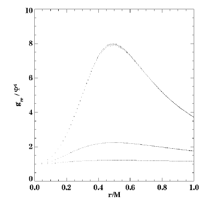
FIG. 20.: We use a scatter plot to show $g_{rr}$ vs. $r$ for all points in a region of the cartesian grid for a geodesically sliced black hole. This scatter plot allows one to see how well spherical symmetry is maintained by eye. From this plot, it is clear that deviations from sphericity occur near the peak at late times, and are fairly small. This figure was generated with $\Delta x=0.05M$, and the slices are shown at $t=0.9M$, $1.8M$, and $2.7M$.

We repeat these tests using our Lax-Wendroff directionally split update method. In Fig. 21 we show a scatter plot of the conformal radial metric function in the neighborhood of its peak at $r=M/2$. We notice that spherical symmetry is obeyed very well despite the fact that this method is a manifestly cartesian method.

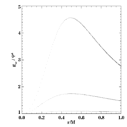
FIG. 21.: We use a scatter plot to show $g_{rr}$ vs $r$ for all points in a region of our cartesian grid for a geodesically sliced black hole. This simulation uses the directionally split Lax-Wendroff solver. This figure was generated with $\Delta x=0.05M$ and slices are shown at $t=0.6M$, $1.5M$, and $2.4M$. We note that even though the method is explicitly split in cartesian directions it maintains excellent spherical symmetry.

In Fig. 22 we show the solution is indeed converging at second order. We measure the convergence order of the hamiltonian constraint and find it is converging at or above $\sigma=2$ during the entire evolution.

FIG. 22.: We show the convergence of the hamiltonian constraint for a geodesically sliced black hole with the flux evolution solved with the directionally split Lax-Wendroff method. We note that convergence is excellent, and points away from the boundary are visually coincident, demonstrating second order convergence of the constraints towards zero away from the boundaries.

B Algebraic Slicings

Algebraic slicing conditions have been used for three dimensional black hole evolutions in the past with a relatively high degree of success, as shown in Refs. [19, 23, 24]. Such slicings typically use Eq. (39) to provide a condition on the lapse. Here we examine the use of such slicings in 3D black hole spacetimes in the BM formulation. We note that such slicings also have been shown under certain conditions to develop coordinate pathologies [45], but we will not investigate those issues here. The main purpose of this section is to compare results of Cactus with previously published results on Schwarzschild black hole evolutions.

The simulations in Refs. [19, 23, 24] used both a diffusion term added to the lapse evolution equation to achieve stability, and an enforced isometry condition, mapping the highly resolved region exterior to the throat into the poorly resolved region interior to the throat. As detailed in Ref. [19], explicit enforcement of this isometry was very important in obtaining accurate long time evolutions of the system, as it allows one to avoid numerical evolution in the coarsely resolved region near the singularity: one simply maps the accurately computed exterior into this region before proceeding to the next time step. Although the algebraic slicing conditions studied actually do obey the isometry operation, and will attempt to preserve it numerically during an evolution, without an explicit isometry operator in the code, large errors will develop inside the throat, causing a code to crash.

An isometry condition could be applied within Cactus, but with the BM system this leads to an additional difficulty in that the isometry conditions on the $D_{ijk}$, $A_{i}$ and $V_{i}$ variables is non-trivial, since these are not tensor quantities. Due to this complication, and due to the promise of alternative techniques such as apparent horizon boundary conditions which do not require isometry conditions, we have currently chosen not to implement an isometry condition in Cactus. Under these conditions it is difficult to achieve the same accuracy and long runtime that were available to an isometry based code, when algebraic slicings are used. We stress that this not a limitation of the code or the formulation of the equations, but merely a sensitivity of such slicings in black hole simulations without an explicit isometry operator. Similar results are obtained, for example, with the “G” code used to generate results in Refs. [19, 23, 24]. Furthermore, we will see in the next section that maximal slicing, which as shown in Ref. [19] does not require the isometry operator, works very well in Cactus.

With those remarks in mind, in Fig. 23 we show the lapse profile in a scatter plot at $t=2.1M$ and $3.5M$ for a “$1+\log$” ($f=1/\alpha$ in Eq. (39)) sliced black hole. Clearly the failure of the lapse to collapse in the center, combined with poor resolution of the consequent gradient in the lapse, will not allow an accurate evolution in this region. Convergence testing this solution at three resolutions, $\Delta x=0.1M$, $\Delta x=0.2M$, and $\Delta x=0.4M$, in this case on a full grid rather than an octant grid, we see that the simulation on the medium resolution grid crashes first, at $t=4.2M$. We note that the lapse is collapsing most quickly at $r=M/2$, indicating that our system is trying to preserve the underlying isometry present in the initial data, as it should.

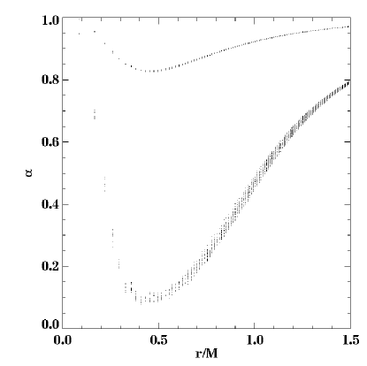
FIG. 23.: We use a scatter plot to show the collapse of the lapse at $t=2.1M$ and $t=3.5M$ for a “1+log” sliced black hole. We note that with this dynamical local slicing, spherical symmetry is not preserved to such a high degree as in the geodesically sliced case, especially near the point of large gradient in the lapse. This inaccuracy in the dipping of the lapse will cause the code to crash shortly after this plot. This data was produced with $\Delta x=0.1M$.

We can understand the nature of the algebraically sliced spacetime without isometry or diffusion by studying its convergence properties. In Fig. 24 we show the convergence of the hamiltonian constraint towards zero at three different resolutions. Several important points in this figure should be noted. Firstly, the very low resolution simulation ($\Delta x=0.4M$, almost the radius of the throat) does not converge from the second slice, $t=2.5M$. As we shall see below, this is because this very low resolution simulation “misses” the isometry, and the lapse collapses, leading to the longest time evolution of the three simulations. We note, however, that at the first two displayed times, the medium and high resolution simulations are converging appropriately, as indicated by the almost coincident lines in Fig. 24. As the medium resolution grid nears its crash time at $t=4.2M$, however, there is no strong evidence of second order convergence in the system near the hole.

FIG. 24.: We show the convergence of the hamiltonian constraint for the “$1+\log$” sliced spacetime. We show 1, 4, and 16 times the hamiltonian constraint at $\Delta x=0.4M$, $0.2M$, and $0.1M$ respectively. We note that the low resolution grid does not converge, and the entire system fails to converge at late times. The medium resolution grid simulation will crash at $t=4.2M$.

Returning to the mystery of the lowest resolution grid, we show in Fig. 25 the evolution of the lapse on the low ($\Delta x=0.4M$) and high ($\Delta x=0.1M$) resolution grids. On the lowest resolution grid the system simply has too few points to obey the isometry, and the lapse collapses uniformly around $r=0$, allowing a long time evolution. The highest resolution grid clearly attempts to obey the isometry, but is destined to fail, due to the small number of points covering the region in $r<M/2$. Thus the two evolutions do not converge towards the same slicing of the spacetime. This is clearly a dangerous feature running a simulation with very poor resolution: it can produce a solution which misses features, but still creates a reasonable looking (and, in this case, longer running) solution than a higher resolution run.

To summarize this subsection, algebraic slicings are convenient and inexpensive singularity avoiding slicing conditions. We have shown that in Cactus they behave as expected, and converge at second order as they should. But they must be used with care. As already shown in Ref. [19], in a spacetime containing a singularity, they can still be very useful if an isometry operator is used to avoid evolving the region near the singularity. Without it, evolution in this region inside the black hole throat is almost impossible in 3D. These slicings should still find use in a number of other circumstances, including use on black holes if precautions are taken near a singularity, if it exists on the grid.

FIG. 25.: We note that on a low enough resolution grid, the isometry condition inherent in the Schwarzschild spacetime, which maintains $\alpha=1$ at the center of the grid, is “missed” so the lapse will collapse everywhere in the center of the grid. Ironically, this under-resolution will allow the low resolution simulation to run considerably longer than the high resolution simulation, but the solution will not converge, of course. Lines are shown with $\Delta x=0.1M$ (solid line) and $0.4M$ (dashed line) at $t=0,1,2,3,$ and $4M$.

C Maximal Slicing

Maximal slicing has long been a favorite slicing condition for numerical relativity. Alas, the maximal slicing condition, Eq.(41), is an elliptic condition for the lapse, which brings with it both a breaking of the hyperbolic system for the lapse and its derivatives and a very large degree of computational complexity.

Solving three-dimensional elliptic equations is far more difficult than solving three-dimensional hyperbolic ones, using much more memory, and taking much more time. For the work in this paper, we use an elliptic solver based on the freely available PETSc software [102], which uses Krylov subspace based matrix methods, such as conjugate gradient, to solve the elliptic conditions which are rewritten as a matrix equation after being cast in finite difference form. The Cactus code has several additional elliptic solvers with various degrees of efficiency and functionality, including several relaxation based solvers, and a parallel multigrid solver developed by B. Brügmann, based on the solver used in Refs. [99, 46].

There are various boundary conditions we can apply to the lapse at the outer boundary when using maximal slicing. For example, we can allow the boundary value of our lapse to change in time, applying the same boundary condition to both the lapse and its derivatives that we apply to all other fields. The “flat” boundary condition used here has the effect of copying the lapse from one point in the interior to the exterior after the maximal equation solve, which causes the lapse to collapse slowly at the outer boundary. We can also use the more traditional approach, which keeps the boundary fixed at some initial value for the entire run. Experience has shown that the best approach in this case is to be initialize $\alpha$ to the (static) Schwarzschild value, and then call the maximal solver, to create the initial lapse profile with the correct spherical outer boundary, as discussed in [19]. This has the added advantage of holding the lapse at the Schwarzschild value near the boundary, reducing evolution of the metric there for some time.

As shown in Ref. [19], unlike with algebraic slicings, one can handle the region inside the throat of the black hole simply by ignoring it. The elliptic maximal lapse was found to collapse rapidly throughout this troublesome region, quickly halting the evolution there. Hence no special precautions, and no isometry operator, are needed to handle this region. We will see the same behavior in Cactus below. Although maximal slicing could be enforced with an isometry condition, as in axisymmetric simulations [83, 103, 97, 104], it is not necessary to do so, and we shall not do so here.

We show here that Cactus runs and converges using maximal slicing by evolving a single black hole on a $100^{3}$ and a $50^{3}$ sized computational grid to $15M$. We look for convergence in the constraints, which should converge to zero, and also in $\rm{tr}K$, which the maximal slicing condition should force to zero.

First we show the behavior of the solution. In Figs. 26 and 27 we show the “collapse of the lapse” and “peak in $g_{rr}$” which are familiar from maximally sliced black hole evolutions in numerical relativity. Due to the singularity avoiding coordinate slicing, we see the lapse collapses towards zero at the center of our grid, which halts evolution, and leads to large proper distances between coordinate points as the exterior evolves, creating large gradients in the metric. We also note that the lapse does collapse at the outer boundary in this simulation, and also that at late times, outer boundary effects are noticeable in $g_{rr}/\psi^{4}$.

FIG. 26.: We show the collapse of the lapse along the $x$–line for a maximally sliced black hole. We note the traditional collapse in the center. We also note that our outer boundary is not held static in this case, and thus the lapse collapses there. This collapse allows evolution with the outer boundary placed nearer the hole than in the static boundary case. This simulation has $\Delta x=0.1M$ and the lapse is shown every $t=0.8M$ from $t=0M$ to $t=14.4M$.

FIG. 27.: We show the growth of the conformal 3-metric $g_{rr}/\psi^{4}$ along the $x$-axis in the maximal slicing case. This figure is the now infamous “grid stretching” figure, and demonstrates the problem which plagues all black hole simulations with singularity avoiding slicing without apparent horizon boundary conditions, namely the explosive growth of the radial metric function. Late time outer boundary problems are also evident in this plot. This simulation has $\Delta x=0.1M$ and the metric is shown every $t=0.8M$ from $t=0M$ to $t=14.4M$.

In Fig. 28 we demonstrate that the system maintains spherical symmetry using the initial lapse of one and allowing the lapse to change at the outer boundary. We note that even on this log scale, and at very small values of the lapse ($\alpha\rightarrow 10^{-4}$) the system maintains excellent spherical symmetry.

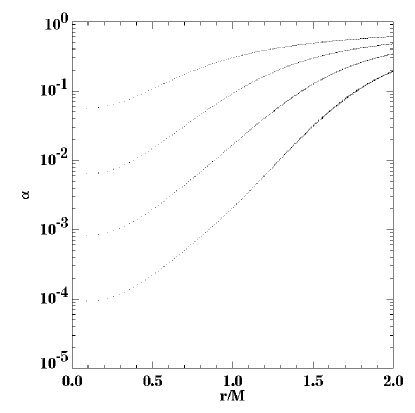
FIG. 28.: We use a scatter plot to show the maintenance of spherical symmetry in the lapse in a maximally sliced black hole. We show the lapse on a log plot, and note that the collapse to very small lapse maintains spherical symmetry to a very high degree. Slices are shown at $t=3.6M$, $7.2M$, $10.8M$, and $14.4M$ The resolution used is $\Delta x=0.1M$.

We emphasize that the growth in $g_{rr}$ is not something we simulate directly. We do not evolve $g_{rr}$, but rather, we evolve cartesian metric functions. These functions must not only display the growth in the radial metric function, but must also contain the decreasing behavior of the angular metric functions. That is $g_{xx}$ must behave like $g_{rr}$ along the $x-$line, but also like $g_{\theta\theta}$ along the $y-$ and $z-$ lines. This leads to an even larger dynamic range in our cartesian metric functions than in the radial or angular metric functions alone. In Fig. 29, we demonstrate this by showing a slice in the $x-y$ plane of $g_{xx}/\psi^{4}$ at $t=14.4M$ for the high resolution ($\Delta x=0.1M$) simulation considered above. It is clear from the figure that the function is growing along the $x-$ axis and dropping along the $y-$ axis, as expected.

FIG. 29.: We show the behavior of the cartesian metric functions by showing a slice in the $x-y$ plane of $g_{xx}/\psi^{4}$ at $t=14.4M$ for the high resolution ($\Delta x=0.1M$) simulation considered above. Note that this function behaves like $g_{rr}$ along the $x-$axis, and $g_{\theta\theta}$ along the $y-$axis.

One obvious question to ask of our simulation is whether or not our maximal slices are actually maximal, in that they keep the ${\rm tr}K$ zero. This condition will be violated by our numerical simulation, but we can check whether the ${\rm tr}K$ converges towards zero. In Fig. 30 we do exactly this. We show the ${\rm tr}K/4$ on the $50^{3}$ $\Delta x=0.2$ grid and ${\rm tr}K$ on the $100^{3}$ $\Delta x=0.1$ grid. If the ${\rm tr}K$ converges to zero at second order we expect these lines to be identical. From Fig. 30 we can clearly see that our evolution converges to a maximal slice at second order.

FIG. 30.: We show the $trK$ at two different resolutions for the maximally sliced case. The dotted line is ${\rm tr}K/4$ calculated with $\Delta x=0.2M$. The solid line is the ${\rm tr}K$ calculated with $\Delta x=0.1M$. Since the ${\rm tr}K=0$ should remain constant in maximal slicing, plotting these two quantities together demonstrates the second order convergence of our solution to the maximally sliced spacetime.

Similarly we can confirm that we are creating a solution to the Einstein equations in our maximally sliced spacetime by testing if the Hamiltonian constraint converges to zero. In Fig. 31 we show one-quarter of the constraint on the $50^{3}$ $\Delta x=0.2$ grid and the constraint on the $100^{3}$ $\Delta x=0.1$ grid. Once again, we see the lines are close to identical visually, strongly indicating second order convergence.

FIG. 31.: We show second order convergence of the hamiltonian constraint in the maximally sliced black hole. We show $H$ at $\Delta x=0.2M$ and $H/4$ at $\Delta x=0.4M$. The fact that the points are visually coincident strongly indicates the system is converging towards a solution of the Einstein equations.

Figs. 30 and 31 demonstrate fairly conclusively that in the regions where our error is larger, our code is converging at second order. However, we note that our simple boundary conditions do lead to small, but non second order convergent, errors at low levels which are not visible in Figs. 30 and 31. We can see these by plotting the ${\rm tr}K$ and hamiltonian at late time (here $t=14.4M$, the final time in Figs. 30 and 31) using a logarithmic $y$ axis, which we do in Fig. 32. Fig. 32 artificially inflates the non second order convergent features due to the boundary, but it is instructive nonetheless. Since these features are on a very low level (several orders of magnitude smaller than the dominant error) they have no real adverse affect on our solution at this time.

FIG. 32.: We show the convergence of ${\rm tr}K$ and the hamiltonian constraint at $t=14.4M$ for the single black hole case considered in Fig. 30 and 31. Here we use a logarithmic $y$ axis, which emphasizes that, at a very low level, the boundary introduces non second order convergent features to the system. Since these effects are several orders of magnitude below the dominant errors, they do not have an adverse effect on our solution (the area with large error is what crashes our code). However, it is clear that our boundaries lead to small, but non second order convergent, effects entering our grid in the less dynamic (spatial) regions.

For the sake of completeness, we also show the failing of convergence of these quantities when our grid is too poorly resolved. In Fig. 33 we show the constraints for a $25^{3}$, $\Delta x=0.4$ run. Since only two points cover the entire initial horizon at this resolution, we cannot reasonably expect a converged answer, and we see that, even though the higher resolution simulations are converging at second order, the low resolution simulation has a worse convergence property. At late times, this effect is mostly due to the lower resolution leading to an earlier crash time on the lowest resolution grid.

FIG. 33.: We repeat the display in Fig. 31, adding a third very low resolution simulation with $\Delta x=0.4M$. We see that the low resolution solution is not converging for $t>12M$, and it will crash soon after the final slice shown here.

We repeat these tests with the outer boundary on the lapse held fixed, which is the condition used previously in Ref. [19]. For this case, we must set the boundary farther away than in the non-fixed case, setting it here initially at $t=15M$, rather than $t=10M$. Additionally, we must use the maximal slicing solver to generate an initial lapse which has the isotropic Schwarzschild form

$$\alpha=\frac{2r-M}{2r+M}$$ (88)

at the outer boundary. This leads to an initial lapse other than one everywhere, as discussed in Ref.[19]. By holding the lapse fixed, we avoid the collapse of the lapse near the boundaries, and therefore evolve for a somewhat longer proper time in the outer region. (We note that with a boundary very far away, as could be provided by some form of adapted mesh structure, the two conditions would be equivalent). Despite this difference, when we evolve the maximally sliced black hole system with the two boundary conditions, we see quantitatively the same behavior in the metric functions.

In Fig. 34 we show the lapse along the x line up to $t=14.4M$, and note it remains fixed at its initial outer boundary value, as expected. Comparing with Fig. 26, we can clearly see that this stops the lapse from collapsing over such a wide portion of the grid, with the lapse at $x=10M$ being around $0.9$ in Fig. 34, and closer to $0.7$ in Fig. 26.

FIG. 34.: We show the collapse of the lapse in the maximally sliced spacetime with the outer boundary held fixed. Note the initial lapse is not one, as it was in Fig. 26, but rather was the result of applying our maximal slicing solver to a lapse which obeys the Schwarzschild lapse outer boundary conditions. The resolution used here was $\Delta x=0.15M$. Slices are shown every $1.2M$ between $t=0M$ and $t=14.4M$.

In Fig. 35 we show the convergence of the ${\rm tr}K$ and hamiltonian constraint to zero at $t=12M$, and note we still achieve second order convergence visually.

FIG. 35.: We show the convergence of the ${\rm tr}K$ and the hamiltonian constraint towards zero at $t=12M$ for the maximally sliced spacetime with a fixed outer boundary. We note that, due to the lower resolution used in this simulation ($\Delta x=0.15$ rather than $0.1$) convergence of the constraints starts to fail near the peak earlier.

D Comparison with ADM Code

In the above sections, we have demonstrated that the BM formalism can generate convergent black hole spacetimes. In this section we confirm that the Cactus ADM integrator is also second order convergent on black hole spacetimes by repeating several of the above tests, and compare ADM results with results from the BM formulation.

In general, we find that the BM and ADM systems generate comparable results, although, as shown below, the ADM system we have implemented will generally run some time longer than the BM system in maximally sliced black hole spacetimes, with large errors appearing first in the BM system. The grid stretching problems ultimately ruins both calculations. We emphasize that this is in not a shortcoming of the BM system; treating the system with advanced methods as described in, for instance, Ref.[61] will allow the BM system (in one dimension) to evolve for significantly longer times than the ADM system, showing a real advantage in using the first order system when combined with advanced numerical techniques. Rather, this demonstrates that when evolving mathematically equivalent systems of equations, on problems such as these black holes that have large gradients, without using numerical methods designed to handle such features, both will fail when gradients become too steep to resolve. The details of how the calculation fails can depend on many factors. Thus for black holes, the present numerical methods applied to to BM system, which only moderately exploit the first order nature (in this case, “flat” boundaries, the Strang split, and the true MacCormack method) are not guaranteed to generate markedly better or longer numerical evolutions than, say, the ADM system with leapfrog.

We return first to the geodesically sliced black hole. In Fig. 36 we repeat the test from Fig. 18, by comparing $g_{rr}/\psi^{4}$ with the analytic Novikov solution, Eq.(VI A). We show the difference at a high resolution ($\Delta x=0.1$) and $1/4$ the difference at a lower resolution, ($\Delta x=0.2$). The points are visually coincident indicating second order convergence on our grid, which we see in general.

FIG. 36.: We show that the ADM integrator in the Cactus code converges to second order against the analytic Novikov solution, repeating the test presented with the BM integrator in Fig. 18. We show the difference between the analytic solution and the computed solution at $\Delta x=0.1$ and one quarter the error at $\Delta x=0.2$. The fact that the points are visually coincident demonstrates second order convergence, which we see on our entire grid.

The most interesting comparison is the maximally sliced black hole. Studies of the three-dimensional maximally sliced black hole with the ADM system have been undertaken in great detail in Ref.[19], so we only treat them briefly here, using the cactus ADM integrator.

In Fig. 37 we show that the BM and ADM system give qualitatively the same behavior at a fixed resolution (since both systems converge at second order, in the limit of infinite resolution they would give identical results). We show the metric function $g_{rr}/\psi^{4}$ every $3M$ between $0M$ and $15M$ with a resolution $\Delta x=0.15$ and a $100^{3}$ grid. We see clearly that the behavior is the same in both cases, although at late times, the two solutions are noticeably different near the peak in $g_{rr}$.

FIG. 37.: We compare $g_{rr}/\psi^{4}$ for a maximally sliced single black hole spacetime evolved with $\Delta x=0.15$ on a $100^{3}$ grid with the ADM and BM integrators. In the ADM system all values are held fixed at the outer boundary, while in the BM system, only the lapse and its derivatives are held static, corresponding to the run in Fig. 34. We show data every $3M$ between $0$ and $15M$ along the $x-$line. We note that both systems exhibit qualitatively the same behavior.

Even though the two solutions in Fig. 37 are different, both solutions are converging to second order, as shown in Figs. 38 and 39. In these figures, we repeat the tests of Figs. 30 and 31 by convergence testing both the ${\rm tr}K$ and the hamiltonian constraint against zero. We see converge close to second order visually in the figures, and everywhere on the grid when measured globally.

FIG. 38.: We repeat the convergence test in Fig.31 with the ADM integrator. We use parameters $\Delta x=0.15$ on a $100^{3}$ grid and measure $H$ at $\Delta x=0.15$ and $H/4$ at $\Delta x=0.3$. We see almost second order convergence visually, and measure a convergence exponent around two over our entire grid. We note the the convergence order drops away from two as we approach the end of our simulation.

FIG. 39.: We repeat the convergence test in Fig.30 with the ADM integrator. We use parameters $\Delta x=0.15$ on a $100^{3}$ grid and measure ${\rm tr}K$ at $\Delta x=0.15$ and ${\rm tr}K/4$ at $\Delta x=0.3$. We see second order convergence visually, and measure a convergence exponent around two over our entire grid.

We finally directly compare the BM and ADM evolutions of the maximally sliced black hole spacetime with parameter $\Delta x=0.15$ on a $100^{3}$ grid, with all fields held fixed at the outer boundary in the ADM system, and the lapse held fixed with other fields having the “copy” boundary conditions in the BM system. We calculate the hamiltonian constraint using Eq. (35) in both the ADM and BM system, constructing the BM $D_{ijk}$ and $V_{i}$ variables from the ADM system with centered finite differences.

In Fig. 40 we can see that for a large part of the run time, the hamiltonian constraint, although different, is of the same order, around $0.1$. However as $t\rightarrow 15M$, the hamiltonian constraint for the BM system around the peak in $g_{rr}$ drops to a larger (absolute) value than the ADM system. This dropping continues, causing the BM system to crash about $4-5M$ before the ADM system with the parameters chosen here.

FIG. 40.: We compare the hamiltonian constraint in the BM and ADM systems for the $\Delta x=0.15$ $100^{3}$ maximally sliced black hole simulation. The hamiltonian constraint is evaluated by Eq.35 in both cases, with the BM $D_{ijk}$ and $V_{i}$ variables constructed from the ADM simulation at every time step. We note that the errors in the constraint are comparable, but at late times, the errors in the BM system are larger near the maximum of the grid stretching. In the simulation shown here, the ADM code will run around $4-5M$ longer than the BM simulation (with crash times around $16M$ and $20M$ at this resolution). We note that the constraints converge to zero in both cases.

E One-D AH Finder as a test of spherical spacetimes.

Since the only black hole spacetimes we treat here are spherical, we can use spherical expressions for the location of the apparent horizon extracted along constant radial lines of the spacetime. Here we choose diagonal lines. We assume the spherical metric has the line element

$$dl^{2}=\psi^{4}(g_{rr}dr^{2}+g_{\theta\theta}d\Omega^{2})\;,$$ (89)

so the outgoing normal has the form

$$s^{a}=\frac{1}{\psi^{2}\sqrt{g_{rr}}}(1,0,0)\;.$$ (90)

We can evaluate the expansion,

$$D_{a}s^{a}+K_{ab}s^{a}s^{b}-trK=$$ (91)

$$\frac{1}{\psi^{2}\sqrt{g_{rr}}}\left(4\frac{\psi_{,r}}{\psi}+\frac{g_{\theta\theta,r}}{g_{\theta\theta}}+\frac{2}{r}\right)-\frac{2K_{\theta\theta}}{\psi^{4}g_{\theta\theta}}$$ (92)

everywhere along this line. The point where the expansion crosses zero defines the apparent horizon. By measuring $\psi^{4}r^{2}g_{\theta\theta}/4M^{2}$ there, we can monitor the horizon area, which should be identically 1 using this normalization.

In Fig. 41 we show the evolution of the apparent horizon area up to $15M$ in the maximally sliced cases discussed above. We can make a crude estimate of how well our horizon is converging by measuring the convergence exponent for its radial location versus time. Although this measure is plagued by oscillations, we see that, on the whole, we have better than second order convergence. As well as a spherical AH finder, determined by finding the zero of Eq.(92), the Cactus code has a parallelized implementation of Gundlach’s Pseudo-spectral apparent horizon finder [105]. Applications of this AH finder during dynamic evolutions will be discussed elsewhere.

FIG. 41.: We show the area of the apparent horizon for the $dx=0.1M$ maximally sliced black hole. The apparent horizon is extracted along the diagonal line.

VII Summary

Hyperbolic formulations of Einstein’s equations have been proposed by a number of groups as a promising tool for numerical relativity [2, 3, 4, 64, 73, 67]. These reformulations of Einstein’s equations have shown great strength in 1D tests[60, 3]. Early versions of the BM hyperbolic formulation [2] were developed into a full 3D code and tested on dynamically sliced flat space [56], leading further to the development of the “H” code which was applied to 3D gravitational wave studies [41]. A 3D version of the Abrahams et al. hyperbolic formulation[64] is also currently under development [69]. But these 3D codes have seen only limited development and application.

In this work we have performed the first systematic and detailed numerical exploration of a 3D hyperbolic formulation of Einstein’s equations on a number of spacetimes of broad interest in physics and astronomy. We developed and tested a full 3D numerical code, called Cactus, which implements the recent and more general BM hyperbolic formulation of Einstein’s equations[3, 4]. With this code, we showed on various dynamically sliced flat space, black hole, and gravitational wave spacetimes that this formulation allows for numerical treatment that is as stable and accurate as the traditional applications of the ADM formulation.

The Cactus code has a modular structure allowing for different formulations of the Einstein equations, including the ADM system, different numerical methods, and many different initial data, gauge, and analysis routines. Cactus is developed on an advanced parallel computational infrastructure, achieving over 66GFlops/sec on a 512 node Cray T3E supercomputer[70, 71]. In this paper, within Cactus we compared Strang split MacCormack and Lax-Wendroff methods, applied to the Bona Massó system, against a leapfrog implementation of the ADM system, and also against previous results obtained from two completely independent 3D codes (the “G” code, based on the ADM formulation, and the “H” code, described above). The numerical methods used were described in detail.

For the 3D black hole spacetimes, we studied (a) geodesically sliced black holes, and compared with the analytic solution of Novikov, (b) algebraic slicings, which have good singularity avoidance properties, (c) and maximal slicing, which is has traditionally been a preferred choice for numerical black hole evolution. On all tests with both the ADM and BM formulation, the code performed well, reproducing previous published results on spherical black hole evolution in 3D [19].

For 3D pure gravitational wave spacetimes, Cactus was tested on the evolution of linearized quadrupole and plane waves against previous results obtained with the “G” and “H” codes, again reproducing results of extensive studies published previously [41]. Cactus was also tested with dynamically sliced Minkowski spacetimes, where quantities such as Riemann invariants were shown to converge to zero.

We also discussed the importance of convergence tests, and detailed a number of techniques we have developed to test convergence of the code. We showed that Cactus is rigorously second order convergent, and we emphasized that convergence tests are important techniques for diagnosing code errors.

We emphasize that although this paper shows many successful applications of a 3D hyperbolic formulation of Einstein’s equations, we have focussed on applying standard numerical methods for flux conservative systems, and on showing that they perform as well as standard methods applied to the ADM system. We have not yet exploited the kinds of advanced numerical methods that can be applied to the eigenfields of a hyperbolic system. Such numerical treatments are ultimately one of the major motivations for using hyperbolic systems in numerical relativity. The application of numerical methods specifically designed for hyperbolic systems (e.g. TVD methods [51, 85]) has produced vast improvements in 1D studies of black holes, and their applications in 3D will are under development. Advanced inner (e.g. on a black hole horizon) and outer (e.g. at the edge of a numerical grid) boundary treatments may also be possible through the use of the eigenfields. The present Cactus code provides an advanced parallel tool for developing and testing such methods.

This paper is the first in an anticipated long series with many collaborators. There are many directions in which research with this code is proceeding. We are currently working on evolution of multiple black hole spacetimes, evolution of strong gravitational waves, 3D apparent horizon boundary conditions, self-gravitating scalar fields, advanced numerical treatments of the characteristic system, and full general relativistic hydrodynamics, among other projects. We expect that future papers will build on this one, continuing to show careful comparisons with analytic solutions, demonstrating rigorous self-convergence, and discussing the effects of boundaries and numerical methods.

We plan to make the code used for the all calculations in this paper publicly available at some point after the publication of this paper, together with the parameter files used to produce the figures and additional color figures and movies that provide more details than it is possible to show in printed form. All this information and instructions on uploading the code will be located at the web address http://cactus.aei-potsdam.mpg.de/.

VIII Acknowledgments

The Cactus code has been developed in the Albert Einstein Institute in Potsdam, Germany, with input from our many collaborators and friends at Washington University in St. Louis, the National Center for Supercomputing Applications in Champaign, Illinois, the University of the Balearic Islands in Mallorca, Spain, and elsewhere. We would like to thank Miguel Alcubierre, Gabrielle Allen, Miguel Angel Aloy, Pete Anninos, Toni Arbona, Steve Brandt, Bernd Brügmann, Dan Bullok, Jaume Carot, Tom Clune, Ying Chen, Greg Daues, Thomas Dramlitsch, Ed Evans, Toni Font, Ian Foster, Tom Goodale, Carsten Gundlach, Peter Hübner, José María Ibáñez, Sai Iyer, Klaus Ketelsen, Szu-Wen Kuo, Gerd Lanferman, Lluis Mas, Richard Matzner, Wolfgang Mertz, Mark Miller, Phillipos Papadopolous, Manuel Panea, Manish Parashar, K.V. Rao, Sirpa Saarinen, Faisal Saied, Paul Saylor, Uli Schwenn, Bernd Schmidt, Bernard Schutz, John Shalf, Hisa-aki Shinkai, Barry Smith, Joan Stela, Wai-Mo Suen, Doug Swesty, Ryoji Takahashi, Kip Thorne, Malcolm Tobias, John Towns, and Ed Wang for help with testing, bug reports and fixes, encouragement, developing thorns, and useful discussions. Without help from all of these people, Cactus would not be nearly as advanced and well tested as it is today.

We would especially like to thank Steve Brandt for providing an early release of the thorn that computes the Riemann invariants. Calculations and development were carried out at the Albert Einstein Institute, the University of the Balearic Islands, and at the Konrad-Zuse Computing Center. C.B. wishes to thank Albert-Einstein-Institut for support by the AEI visitor program. This work is supported by the DGICyT of Spain under project PB-94-1177 and also by NSF grant INT94-14185. This work also benefitted greatly from collaborations funded by NASA-NCCS5-153.

Appendix A: The Conformally Rescaled BM Equations

Here we detail the equations modifications necessary to take into account a static conformal factor for the metric. We will evolve a “conformal” metric $g_{ij}$ related to the physical metric $\hat{g}_{ij}$ by the conformal factor $\psi$:

$${\hat{g}}_{ij}=\psi^{4}\;g_{ij}\;.$$ (93)

We will keep the same formal definitions for the BM variables:

$$D_{kij} = \frac{1}{2}\partial_{k}g_{ij}\;,$$ (94)

$$V_{i} = {D_{ir}}^{r}-{D^{r}}_{ri}\;,$$ (95)

where indices are raised with $g^{ij}$ and lowered with $g_{ij}$.

With these definitions, the physical BM variables relate to the conformal ones by

$${\hat{D}}_{kij} = \psi^{4}(D_{kij}+2\psi_{k}g_{ij})\;,$$ (96)

$${\hat{V}}_{i} = V_{i}+4\psi_{i}\;.$$ (97)

We also introduce the following notation for the derivatives of the conformal factor

$$\psi_{i} = \frac{\partial_{i}\psi}{\psi}\;,$$ (98)

$$\psi_{ij} = \frac{\partial_{i}\partial_{j}\psi}{\psi}\;.$$ (99)

The Christoffel symbols relate by

$$\hat{\Gamma}^{k}_{\;ij}=\Gamma^{k}_{\;ij}+2\;\delta^{k}_{i}\;{\psi_{j}\over\psi}+2\;\delta^{k}_{j}\;{\psi_{i}\over\psi}-2\;{\psi^{k}\over\psi}\;g_{ij}\;,$$ (100)

and the Ricci tensor by

$$\hat{R}_{ij}=R_{ij}-Y_{ij}-Y_{k}^{\;k}g_{ij}\;,$$ (101)

where we define

$$Y_{ij}=-\psi^{2}\;(\psi^{-2})_{;i;j}+2\;{\psi^{k}\over\psi}{\psi_{k}\over\psi}\;g_{ij}$$ (102)

with covariant derivatives computed using $\Gamma^{k}_{\;ij}$. Thus,

$$Y_{ij}=2g_{ij}\psi^{k}\psi_{k}+2(\psi_{ij}-\psi_{r}{\Gamma^{r}}_{ij}-3\psi_{i}\psi_{j})\;.$$ (103)

We can then derive a modified set of fluxes (note that the flux for the extrinsic curvature does not change):

$$F^{k}_{-}g_{ij} = 0\;,$$ (104)

$$F^{k}_{-}\alpha = 0\;,$$ (105)

$$F^{k}_{-}K_{ij} = -\beta^{k}\,K_{ij}+\alpha\;[\;D^{k}_{ij}-n/2\;V^{k}\;g_{ij}$$ (108)

$$+1/2\;\delta^{k}_{i}\;(A_{j}+2\,V_{j}-D_{jr}^{\;\;r})$$

$$+1/2\;\delta^{k}_{j}\;(A_{i}+2\,V_{i}-D_{ir}^{\;\;r})\;]\;,$$

$$F^{k}_{-}D_{kij} = -\beta^{r}(D_{rij}+2\psi_{r}g_{ij})+\alpha\;(K_{ij}/\psi^{4}-s_{ij})\;,$$ (109)

$$F^{k}_{-}A_{k} = -\beta^{r}A_{r}+\alpha\;Q\;,$$ (110)

$$F^{k}_{-}V_{i} = -\beta^{k}(V_{i}+4\psi_{i})+B^{k}_{\;i}-B_{i}^{\;k}\;.$$ (111)

The modified sources are:

$$S_{-}g_{ij} = -2\;\alpha\;(K_{ij}/\psi^{4}-s_{ij})$$ (113)

$$+2\beta^{r}\,(D_{rij}+2\psi_{r}g_{ij})\;,$$

$$S_{-}\alpha = -\alpha^{2}\;Q+\alpha\beta^{r}\,A_{r}\;,$$ (114)

$$S_{-}K_{ij} = 2(K_{ir}B_{j}^{\;r}+K_{jr}B_{i}^{\;r}-K_{ij}B_{r}^{\;r})$$ (124)

$$+\alpha\;[\;-^{(4)}R_{ij}+(-2K_{i}^{\;k}K_{kj}+tr\,K\;K_{ij})/\psi^{4}$$

$$\;\;\;\;-\Gamma^{k}_{\;ri}\Gamma^{r}_{\;kj}+2D_{ik}^{\;\;r}D_{rj}^{\;\;k}+2D_{jk}^{\;\;r}D_{ri}^{\;\;k}+\Gamma^{k}_{\;kr}\Gamma^{r}_{\;ij}$$

$$\;\;\;\;-(2\,D_{kr}^{\;\;k}-A_{r})(D_{ij}^{\;\;r}+D_{ji}^{\;\;r})$$

$$\;\;\;\;+A_{i}(V_{j}-1/2\;D_{jk}^{\;\;k})+A_{j}(V_{i}-1/2\;D_{ik}^{\;\;k})$$

$$\;\;\;\;+A_{j}(V_{i}-1/2\;D_{ik}^{\;\;k})-nV^{k}D_{kij}\;]$$

$$+n/4\;\alpha g_{ij}\;[\;-D_{k}^{\;rs}\Gamma^{k}_{\;rs}+D_{kr}^{\;\;r}D^{ks}_{\;\;s}-2\,V^{k}A_{k}$$

$$\;\;\;\;+(K^{rs}K_{rs}-(tr\,K)^{2})/\psi^{4}+2\alpha^{2}\;G^{00}\;]$$

$$-Y_{ij}+2A_{i}\psi_{j}+2A_{j}\psi_{i}$$

$$+g_{ij}\;[(n\!-\!1)Y^{k}_{\;k}-2A^{k}\psi_{k}]\;,$$

$$S_{-}D_{kij} = 0\;,$$ (125)

$$S_{-}A_{k} = 0\;,$$ (126)

$$S_{-}V_{i} = \alpha^{2}\;G^{0}_{\;i}+\alpha/\psi^{4}[\;A_{r}(K^{r}_{\;i}-tr\,K\;\delta^{r}_{i})$$ (131)

$$+K^{r}_{\;s}(D_{ir}^{\;\;s}-2D_{ri}^{\;\;s})-K^{r}_{\;i}(D_{rs}^{\;\;s}-2D_{sr}^{\;\;s})$$

$$-2\psi_{r}\;(3K^{r}_{\;k}-tr\,K\;\delta^{r}_{k})\;]$$

$$+2(B_{i}^{\;r}-\delta_{i}^{r}\;tr\,B)\;V_{r}+2(D_{ri}^{\;\;s}-\delta^{s}_{i}\;D^{j}_{\;jr})B^{r}_{\;s}$$

$$+4{B_{i}}^{r}\psi_{r}-4trB\psi_{i}\;.$$

Finally, our algebraic slicing condition becomes

$$Q=f(\alpha)\;tr\,K\;/\psi^{4}\;.$$ (132)

REFERENCES

- [1] J. Massó and P. Walker, (1998), in preparation.
- [2] C. Bona and J. Massó, Phys. Rev. Lett. 68, 1097 (1992).
- [3] C. Bona, J. Massó, E. Seidel, and J. Stela, Phys. Rev. Lett. 75, 600 (1995).
- [4] C. Bona, J. Massó, E. Seidel, and J. Stela, Phys. Rev. D 56, 3405 (1997).
- [5] Éanna É. Flanagan and S. A. Hughes, gr-qc/9710129, (1997).
- [6] Éanna É. Flanagan and S. A. Hughes, gr-qc/9701039, (1997).
- [7] A. M. Abrahams et al., Physical Review Letters 80, 1812 (1998), gr-qc/9709082.
- [8] G. B. Cook et al., (1997), gr-qc/9711078.
- [9] R. Gomez et al., (1998), gr-qc/9801069.
- [10] G. Mathews and J. Wilson, Astrophysical Journal 482, 929 (1997).
- [11] M. Ruffert, M. Rampp, and H.-T. Janka, Astron. Astrophys. , to appear. astro-ph/9611056.
- [12] M. Ruffert, H.-T. Janka, W. Keil, and G. Schäfer, in Proc. of the 17th Texas Symposium on Relativistic Astrophysics (World Scientific, Singapore, 1995).
- [13] K.-I. Oohara and T. Nakamura, in Relativistic Gravitation and Gravitational Radiation, edited by J.-P. Lasota and J.-A. Marck (Cambridge University Press, Cambridge, England, 1997).
- [14] M. Choptuik, Phys. Rev. Lett. 70, 9 (1993).
- [15] C. Gundlach, To appear in Adv. Theor. Math. Phys (1998), gr-qc/9712084.
- [16] A. Abrahams and C. Evans, Phys. Rev. Lett. 70, 2980 (1993).
- [17] C. Gundlach, (1998), gr-qc/9710066.
- [18] P. Anninos, J. Massó, E. Seidel, and W.-M. Suen, Physics World 9, 43 (1996).
- [19] P. Anninos, K. Camarda, J. Massó, E. Seidel, W.-M. Suen, and J. Towns, Phys. Rev. D 52, 2059 (1995).
- [20] B. Brügmann, Phys. Rev. D 54, (1996).
- [21] P. Anninos, D. Hobill, E. Seidel, L. Smarr, and W.-M. Suen, Phys. Rev. Lett. 71, 2851 (1993).
- [22] P. Anninos, D. Hobill, E. Seidel, L. Smarr, and W.-M. Suen, Phys. Rev. D 52, 2044 (1995).
- [23] K. Camarda, Ph.D. thesis, University of Illinois at Urbana-Champaign, Urbana, Illinois, 1998.
- [24] K. Camarda and E. Seidel, Phys. Rev. D 57, 3204 (1998), gr-qc/9709075.
- [25] G. Allen, K. Camarda, and E. Seidel, (1998), in preparation.
- [26] S. L. Shapiro and S. A. Teukolsky, in Dynamical Spacetimes and Numerical Relativity, edited by J. M. Centrella (Cambridge University Press, Cambridge, England, 1986), pp. 74–100.
- [27] R. H. Price and J. Pullin, Phys. Rev. Lett. 72, 3297 (1994).
- [28] P. Anninos, R. H. Price, J. Pullin, E. Seidel, and W.-M. Suen, Phys. Rev. D 52, 4462 (1995).
- [29] A. Abrahams and R. Price, Phys. Rev. D 53, 1972 (1996).
- [30] J. Baker, A. Abrahams, P. Anninos, S. Brandt, R. Price, J. Pullin, and E. Seidel, Phys. Rev. D 55, 829 (1997).
- [31] R. J. Gleiser, C. O. Nicasio, R. H. Price, and J. Pullin, Physical Review Letters 77, 4483 (1996).
- [32] L. Rezzolla, A. M. Abrahams, T. W. Baumgarte, G. B. Cook, M. A. Scheel, S. L. Shapiro, and S. A. Teukolsky, Phys. Rev. D 57, 1084 (1998).
- [33] M. Berger and J. Oliger, Journal of Computational Physics 53, 484 (1984).
- [34] L. A. Wild, Ph.D. thesis, University of Wales, 1996.
- [35] P. Papadapoulos, E. Seidel, and L. Wild, Physical Review D (1998), submitted, gr-qc/9802069.
- [36] E. Seidel and W.-M. Suen, Phys. Rev. Lett. 69, 1845 (1992).
- [37] P. Anninos, G. Daues, J. Massó, E. Seidel, and W.-M. Suen, Phys. Rev. D 51, 5562 (1995).
- [38] M. A. Scheel, S. L. Shapiro, and S. A. Teukolsky, Phys. Rev. D 51, 4208 (1995).
- [39] R. Marsa and M. Choptuik, Phys Rev D 54, 4929 (1996).
- [40] G. E. Daues, Ph.D. thesis, Washington University, St. Louis, Missouri, 1996.
- [41] P. Anninos, J. Massó, E. Seidel, W.-M. Suen, and M. Tobias, Phys. Rev. D 56, 842 (1997).
- [42] P. Anninos, J. Massó, E. Seidel, W.-M. Suen, and M. Tobias, Phys. Rev. D 54, 6544 (1996).
- [43] J. Balakrishna, G. Daues, E. Seidel, W.-M. Suen, M. Tobias, and E. Wang, Class. Quant. Grav. 13, L135 (1996).
- [44] M. Alcubierre, Phys. Rev. D 55, 5981 (1997).
- [45] M. Alcubierre and J. Massó, Phys. Rev. D Rapid Comm., to appear. gr-qc/9709024.
- [46] B. Brügmann, (1997), gr-qc/9708035.
- [47] R. Gomez, L. Lehner, R. Marsa, and J. Winicour, (1997), gr-qc/9710138.
- [48] J. York, in Sources of Gravitational Radiation, edited by L. Smarr (Cambridge University Press, Cambridge, England, 1979).
- [49] H. Friedrich, Class. Quant. Grav. 13, 1451 (1996).
- [50] O. Reula, Living Reviews in Relativity 1, (1998).
- [51] R. J. Leveque, Numerical Methods for Conservation Laws (Birkhauser Verlag, Basel, 1992).
- [52] Y. Choquet-Bruhat and T. Ruggeri, Comm. Math. Phys 89, 269 (1983).
- [53] H. Friedrich, Comm. Math. Phys. 100, 1525 (1985).
- [54] C. Bona and J. Massó, Phys. Rev. D 38, 2419 (1988).
- [55] C. Bona and J. Massó, Phys. Rev. D 40, 1022 (1989).
- [56] J. Massó, Ph.D. thesis, University of the Balearic Islands, 1992.
- [57] C. Bona and J. Massó, in Approaches to Numerical Relativity, edited by R. D’Inverno (Cambridge University Press, Cambridge, England, 1992).
- [58] R. Gjertsen, J. Massó, M. Nardulli, E. Seidel, J. Shalf, and D. Weber, Forefronts 11, (1996), cornell Theory Center.
- [59] S. Kuo, M. Winslett, K. Seamons, Y. Chen, Y. Cho, and M. Subramaniam, in Proceedings of the SIAM Conference on Parallel Processing for Scientific Computing (SIAM, Minneapolis, MN, 1997).
- [60] C. Bona, J. Massó, and J. Stela, Phys. Rev. D 51, 1639 (1995).
- [61] A. Arbona, C. Bona, J. Massó, and J. Stela, In preparation (1998).
- [62] S. Fritelli and O. Reula, Commun. Math. Phys. 166, 221 (1994).
- [63] Y. Choquet-Bruhat and J. York, C. R. Acad. Sc. Paris 321, 1089 (1995).
- [64] A. Abrahams, A. Anderson, Y. Choquet-Bruhat, and J. York, Phys. Rev. Lett. 75, 3377 (1995).
- [65] S. Fritelli and O. Reula, Phys. Rev. Lett. 75, 4667 (1995).
- [66] M. H. van Putten and D. Eardley, Phys. Rev. D 53, 3056 (1996).
- [67] A. Abrahams, A. Anderson, Y. Choquet-Bruhat, and J. York, Class.Quant.Grav A9 (1997).
- [68] M. Scheel, T. Baumgarte, G. Cook, S. Shapiro, and S. Teukolsky, Phys. Rev. D 56, 6320 (1997).
- [69] G. Cook and M. Scheel, private communication.
- [70] T. Clune, J. Massó, M. Miller, and P. Walker, Technical report, National Center for Supercomputing Applications, (unpublished), in preparation.
- [71] P. Walker, Technical report, National Center for Supercomputing Applications, (unpublished), in preparation.
- [72] W. H. Press, B. P. Flannery, S. A. Teukolsky, and W. T. Vetterling, Numerical Recipes (Cambridge University Press, Cambridge, England, 1986).
- [73] A. Abrahams, A. Anderson, Y. Choquet-Bruhat, and J. York, C.R. Acad. Sci. Paris 835 (1996).
- [74] The Message Passing Interface (MPI) standard, http://www.ncs.anl.gov/mpi/.
- [75] M. Parashar and J. C. Browne, Proceedings of the International Conference for High Performance Computing 22 (1995).
- [76] M. Parashar and J. C. Browne, Proceedings of the Annual Hawaii International Conference on System Sciences 604 (1996).
- [77] P. Anninos, D. Hobill, E. Seidel, and W.-M. Suen, Proceedings of the Sixth Canadian Conference on General Relativity and Relativistic Astrophysics (Fields Institute Comunications, 1996), in press.
- [78] G. Allen, K. Camarda, and E. Seidel, in preparation.
- [79] N. Bishop, R. Gomez, L. Lehner, and J. Winicour, Phys. Rev. D 52, (1997).
- [80] P. Hübner, gr-qc/9804065 (1998).
- [81] P. Hübner, Phys. Rev. D 53, 701 (1996).
- [82] J. Frauendiener, gr-qc/971250 and gr-qc/9712052 (1997).
- [83] A. Abrahams, D. Bernstein, D. Hobill, E. Seidel, and L. Smarr, Phys. Rev. D 45, 3544 (1992).
- [84] A. Arbona, C. Bona, J. Carot, L. Mas, J. Massó, and J. Stela, Phys. Rev. D 57, 2397 (1998).
- [85] C. Bona, in Relativity and Scientific Computing, edited by F. Hehl (Springer-Verlag, Berlin, 1996).
- [86] H. C. Yee, Computational Fluid Dynamics (von Karman Institute for Fluid Dynamics, NASA Ames Research Center, CA, 1989).
- [87] P. Walker, Ph.D. thesis, University of Illinois at Urbana-Champaign, Urbana, Illinois, 1998, in preparation.
- [88] M. Choptuik, Phys. Rev. D 44, 3124 (1991).
- [89] L. Gunnarsen, H. Shinkai, and K. Maeda, Class. Quant. Grav. 12, 133 (1995).
- [90] P. Anninos, K. Camarda, J. Massó, E. Seidel, W.-M. Suen, M. Tobias, and J. Towns, in The Seventh Marcel Grossmann Meeting: On Recent Developments in Theoretical and Experimental General Relativity, Gravitation, and Relativistic Field Theories, edited by R. T. Jantzen, G. M. Keiser, and R. Ruffini (World Scientific, Singapore, 1996), pp. 644–647.
- [91] U. Yurtsever, Phys. Rev. D 37, 2790 (1988).
- [92] U. Yurtsever, Phys. Rev. D 38, 1731 (1988).
- [93] M. Shibata and T. Nakamura, Phys. Rev. D 52, 5428 (1995).
- [94] S. Teukolsky, Phys. Rev. D 26, 745 (1982).
- [95] C. Evans, in Dynamical Spacetimes and Numerical Relativity, edited by J. Centrella (Cambridge University Press, Cambridge, England, 1986), pp. 3–39.
- [96] K. Camarda and E. Seidel, in preparation.
- [97] D. Bernstein, D. Hobill, E. Seidel, L. Smarr, and J. Towns, Phys. Rev. D 50, 5000 (1994).
- [98] S. Brandt and E. Seidel, Phys. Rev. D 52, 856 (1995).
- [99] S. Brandt and B. Brügmann, Phys. Rev. Lett. 78, 3606 (1997).
- [100] C. W. Misner, K. S. Thorne, and J. A. Wheeler, Gravitation (W. H. Freeman, San Francisco, 1973).
- [101] B. Brügmann, private communication.
- [102] S. Balay, W. Gropp, L. C. McInnes, and B. Smith, PETSc - The Portable, Extensible Toolkit for Scientific Compuation, 1998, http://www.mcs.anl.gov/petsc/.
- [103] D. Bernstein, Ph.D. thesis, University of Illinois Urbana-Champaign, 1993.
- [104] P. Anninos, D. Bernstein, D. Hobill, E. Seidel, L. Smarr, and J. Towns, in Computational Astrophysics: Gas Dynamics and Particle Methods, edited by W. Benz, J. Barnes, E. Muller, and M. Norman (Springer-Verlag, New York, 1997), in press.
- [105] C. Gundlach, Phys. Rev. D 57, 863 (1998).