Perturbations in the Kerr-Newman Dilatonic Black Hole Background:
Maxwell Waves, the Dilaton Background and Gravitational Lensing

Abstract

In this paper we continue the analysis of one of our previous papers and study the affect of the existence of a non-trivial dilaton background on the propagation of electromagnetic waves in the Kerr-Newman dilatonic black hole space-time. For this purpose we again employ the double expansion in both the background electric charge and the wave parameters of the relevant quantities in the Newman-Penrose formalism and then identify the first order at which the dilaton background enters Maxwell equations. We then assume that gravitational and dilatonic waves are negligible (at that order in the charge parameter) with respect to electromagnetic waves and argue that this condition is consistent with the solutions already found in the previous paper. Explicit expressions are given for the asymptotic behaviour of scattered waves, and a simple physical model is proposed in order to test the effects. An expression for the relative intensity is obtained for Reissner-Nordström dilaton black holes using geometrical optics. A comparison with the approximation of geometrical optics for Kerr-Newman dilaton black holes shows that at the order to which the calculations are carried out gravitational lensing of optical images cannot probe the dilaton background.

I Introduction

In Ref. [1] we started from the low energy effective action describing the Einstein-Maxwell theory interacting with a dilaton of arbitrary coupling constant $a$ in four dimensions (we always set $c=G=1$ unless differently stated),

$$S={1\over 16\,\pi}\,\int d^{4}x\,\sqrt{-g}\,\left[R-{1\over 2}\,(\nabla\phi)^{2}-e^{-a\,\phi}\,F^{2}\right]\ ,$$ (1)

and, on expanding the fields in terms of the charge-to-mass ratio $Q/M$ of the source, we obtained the static solution of the field equations corresponding to a Kerr-Newman dilatonic (KND) black hole rotating with arbitrary angular momentum. Our solution reduces to the Kerr-Newman (KN) metric (see e.g. [2]) for $a=0$ and to the Kaluza-Klein solution [3] for $a=\sqrt{3}$, but differs from the exact Reissner-Nordström dilatonic (RND) black hole [4] in the zero angular momentum limit [5]. In Ref. [6], to which we refer for all the definitions and notation, we used these solutions to write the wave equations for the various field modes. Our method is to double expand each field in powers of the electric charge and the wave parameter. Substituting these expansions into Maxwell’s equations, the dilaton equation and Einstein’s equations then give (inhomogeneous) wave equations for the coefficients of the expansion to any desired accuracy.

We have already given explicit expressions for Maxwell’s equations for the coefficients linear in the wave parameter for the three lowest orders of the charge parameter and have found the asymptotic form of the solutions linear in the wave and charge parameters (order $(1,1)$ in the notation of [6]). The latter correspond to Maxwell waves produced by dilaton waves scattered by the static electromagnetic background.

In this paper we analyze the Maxwell waves produced by the scattering of electromagnetic waves by the static dilaton background which emerge at order $(1,2)$. Since Maxwell’s equations at order $(1,2)$ contain waves of all kinds [7], finding analytic solutions seems an intractable problem. We thus pursue a suggestion already introduced in [6] and assume that the dilaton waves and the gravitational waves are negligible with respect to Maxwell waves which allows us to greatly simplify the equations for electromagnetic waves. In section II we check the consistency of such a working ansatz and argue that it is valid at order (1,2) when one considers the solutions at order $(1,1)$ which we have found in [6]. In section III we compute the asymptotic behaviour at large distance from the hole of both outgoing and ingoing modes of the reduced Maxwell equations and propose a physical onset to detect the dilaton background in a binary system from the scattered pattern of radiation emitted by the star companion. In section IV we show an alternative way of computing the variation of the flux of a null wave scattered by RND and KND black holes in the approximation of geometrical optics. This approach reflects the qualitatively different natures of the two kinds of metrics and proves that light paths are not affected be the dilaton background in KND at the computed order in the charge-to-mass expansion. We also compare this result with the wave approach of the previous sections.

II Wave equations at order (1,2)

We employ the double expansion of perturbations [6] of the static solution given in Ref. [1] in order to write the wave equations for the various field modes,

$$\phi(t,r,\theta,\varphi)=\sum\limits_{p,n}\,g^{p}\,Q^{n}\,\phi^{(p,n)}$$ (2)

$$\phi_{i}(t,r,\theta,\varphi)=\sum\limits_{p,n}\,g^{p}\,Q^{n}\,\phi^{(p,n)}_{i}\ ,\ \ \ i=0,1,2$$ (3)

$$G(t,r,\theta,\varphi)=\sum\limits_{p,n}\,g^{p}\,Q^{n}\,G^{(p,n)}\ ,$$ (4)

where $g$ is the same wave parameter for the dilaton ($\phi$), Maxwell ($\phi_{i}$) and gravitational (collectively denoted by $G$) field quantities. Of course, we will only study the linear ($p=1$) case and set $g=1$ from now on. We assume the linear perturbations have the following time and azimuthal dependence

$$\phi^{(1,n)}(t,r,\theta,\varphi) = k_{d}\,e^{i\,\bar{\omega}\,t+i\,m\,\varphi}\,\phi^{(1,n)}(r,\theta)$$ (5)

$$\phi_{i}^{(1,n)}(t,r,\theta,\varphi) = k_{EM}\,e^{i\,\bar{\omega}\,t+i\,m\,\varphi}\,\phi_{i}^{(1,n)}(r,\theta)\ ,\ \ \ i=0,1,2$$ (6)

$$G^{(1,n)}(t,r,\theta,\varphi) = k_{G}\,e^{i\,\bar{\omega}\,t+i\,m\,\varphi}\,G^{(1,n)}(r,\theta)\ ,$$ (7)

where $k_{d}$, $k_{EM}$ and $k_{G}$ are parameters. We recall here that each function of $r$ and $\theta$ on the R.H.S.s above implicitly carries an extra integer index, $m$, anda continuous dependence on the frequency $\bar{\omega}$.

As shown in [6], it is at order $(1,2)$ that the effect induced by the dilaton background appears in all of the equations. Since at this order the different kinds of waves do not disentangle even for $a=0$ [7], we need a working ansatz to obtain a manageable set of equations. As already suggested in [6], we shall tentatively assume

$$k_{EM}\gg k_{d},k_{G}\ ,$$ (8)

and neglect both dilaton and gravitational waves with respect to Maxwell waves. This hypothesis is equivalent to assuming the existence of (space-time) boundary conditions such that the gravitational and dilaton contents of the wave field are negligibly small when compared to the electromagnetic sources, a condition that is not automatically consistent and will be checked in the following for the whole set of field equations.

For completeness, we observe that, in case $k_{EM}\sim k_{d},k_{G}$ the leading contributions to the electromagnetic waves come from order (1,1) and have already been found in [6]. Therefore the present notes together with [6] should cover most of the leading order electromagnetic physics that one can extract from the study of classical waves on the KND background.

A Gravitational equations

In [6] we considered the gravitational field to be determined by the following three non vacuum equations in the Newman-Penrose (NP) formalism,

$$(\hat{\delta}^{*}-4\,\tilde{\alpha}+\pi)\,\Psi_{0}-(\hat{D}-4\,\tilde{\rho}-2\,\epsilon)\,\Psi_{1}-3\,\kappa\,\Psi_{2}=(\hat{\delta}+\pi^{*}-2\,\tilde{\alpha}^{*}-2\,\beta)\,R_{11}$$ (9)

$$-(\hat{D}-2\,\epsilon-2\,\tilde{\rho}^{*})\,R_{12}+2\,\sigma\,\,R_{21}-2\,\kappa\,\,R_{22}-\kappa^{*}\,\,R_{13}$$ (10)

(11)

$$(\hat{\Delta}-4\,\gamma+\mu)\,\Psi_{0}-(\hat{\delta}-4\,\tau-2\,\beta)\,\Psi_{1}-3\,\sigma\,\Psi_{2}=(\hat{\delta}+2\,\pi^{*}-2\,\beta)\,R_{12}$$ (12)

$$-(\hat{D}-2\,\epsilon+2\,\epsilon^{*}-\tilde{\rho}^{*})\,R_{13}-\lambda^{*}\,\,R_{11}-2\,\sigma\,\,R_{22}-2\,\kappa\,\,R_{23}$$ (13)

(14)

$$(\hat{D}-\tilde{\rho}-\tilde{\rho}^{*}-3\,\epsilon+\epsilon^{*})\,\sigma-(\hat{\delta}-\tau+\pi^{*}-\tilde{\alpha}^{*}-3\,\beta)\,\kappa-\Psi_{0}=0\ .$$ (15)

The Ricci tensor terms are given by the Einstein field equations,

$$R_{ab}={1\over{2}}\,\phi_{|a}\,\phi_{|b}+2\,T^{EM}_{ab}\ ,$$ (16)

and the electromagnetic energy-momentum tensor is

$$T^{EM}_{ij}=e^{-a\,\phi}\,\left[F_{ik}\,F^{k}_{j}-{1\over{4}}\,g_{ij}\,F^{2}\right]\equiv e^{-a\,\phi}\,F\,F\,g\,\left(1-{1\over{4}}\,g\,g\right)\ ,$$ (17)

where, in the far R.H.S. we omit indices for brevity, so that $F$ represents any of the components of the Maxwell field strength and $g$ (not to be confused with the wave parameter that we have set to 1) any component of the metric tensor.

For the purpose of further simplifying the expressions, we also observe that Eq. (15) above can be formally rewritten as

$${\cal G}\,G={\cal G}\,R\ ,$$ (18)

where ${\cal G}$ represents any differential operator with coefficients which depend on gravitational quantities only, $G$ represents any gravitational quantity and $R$ here stands for any component of the Ricci tensor. On omitting vanishing terms one then finds that at order $(1,2)$ Eq. (15) can be written

$$k_{G}\,\left({\cal G}^{(0,0)}\,G^{(1,2)}+{\cal G}^{(0,2)}\,G^{(1,0)}+{\cal G}^{(1,0)}\,G^{(0,2)}+{\cal G}^{(1,2)}\,G^{(0,0)}\right) = {\cal G}^{(0,0)}\,R^{(1,2)}+k_{G}\,{\cal G}^{(1,0)}\,R^{(0,2)}\ ,$$ (19)

where

$$R^{(0,2)} = 2\,F^{(0,1)}\,F^{(0,1)}\,g^{(0,0)}\,\left(1-{1\over{4}}\,g^{(0,0)}\,g^{(0,0)}\right)$$ (20)

$$R^{(1,2)} = k_{d}\,\phi_{|a}^{(1,0)}\,\phi_{|b}^{(0,2)}+4\,k_{EM}\,F^{(0,1)}\,F^{(1,1)}\,g^{(0,0)}\,\left(1-{1\over{4}}\,g^{(0,0)}\,g^{(0,0)}\right)$$ (22)

$$+2\,F^{(0,1)}\,F^{(0,1)}\,\left[k_{G}\,g^{(1,0)}\,\left(1-{3\over 4}\,g^{(0,0)}\,g^{(0,0)}\right)-a\,k_{d}\,\phi^{(1,0)}\,g^{(0,0)}\right]\ .$$

If we now apply our ansatz, Eq. (8), and neglect any terms proportional to $k_{G}$, $k_{d}$ with respect to terms proportional to $k_{EM}$, we find that the third equation in Eq. (15) is not affected, since it does not explicitly depend on electromagnetic waves, whilst the first and second equations can apparently be reduced to

$$0\simeq{\cal G}^{(0,0)}\,R^{(1,2)}\simeq 4\,k_{EM}\,{\cal G}^{(0,0)}\,F^{(0,1)}\,F^{(1,1)}\,g^{(0,0)}\,\left(1-{1\over{4}}\,g^{(0,0)}\,g^{(0,0)}\right)\,\ .$$ (23)

These would be undesired constraints for the solutions of Maxwell’s equations at order $(1,1)$ which we have already found in [6]. However, we recall here that those (particular) solutions of the inhomogeneous equations which we denoted by $\phi_{i}^{(1,1)}$ in Section IV of [6] are proportional to $k_{d}/k_{EM}$. Therefore $F^{(1,1)}\sim k_{d}/k_{EM}$ and, on substituting into the R.H.S. of Eq. (23), one obtains expressions which are indeed proportional to $k_{d}$. Thus it is not consistent to neglect terms proportional to $k_{G}$, $k_{d}$ in Eq. (19), since there is no term proportional to $k_{EM}$ with respect to which they are small and none of the above gravitational equations is affected by the approximation in Eq. (8). They are and remain three independent equations for the gravitational quantities $G^{(1,2)}$.

Of course, Eq. (19) is so involved that obtaining an analytic solution appears to be unlikely.

B Dilaton equation

The equation for the dilaton field in the NP tetrad components is

$$\left[\hat{D}\,\hat{\Delta}+\hat{\Delta}\,\hat{D}-\hat{\delta}\,\hat{\delta}^{*}-\hat{\delta}^{*}\,\hat{\delta}+(\epsilon+\epsilon^{*}-\tilde{\rho}-\tilde{\rho}^{*})\,\hat{\Delta}+(\mu+\mu^{*}-\gamma-\gamma^{*})\,\hat{D}\right.$$ (24)

$$\left.\phantom{[}+(\tau-\pi^{*}+\tilde{\alpha}^{*}-\beta)\,\hat{\delta}^{*}+(\tau^{*}-\pi+\tilde{\alpha}-\beta^{*})\,\hat{\delta}\right]\phi=-a\,e^{-a\,\phi}\,F^{2}\ ,$$ (25)

and can be rewritten in analogy with Eq. (18) as

$${\cal G}\,\phi=-a\,e^{-a\,\phi}\,F\,F\,g\,g\ .$$ (26)

At order $(1,2)$ and neglecting terms which vanish identically, one then has

$$k_{d}\,{\cal G}^{(0,0)}\,\phi^{(1,2)}+k_{d}\,{\cal G}^{(0,2)}\,\phi^{(1,0)}+k_{G}\,{\cal G}^{(1,0)}\,\phi^{(0,2)} = -2\,a\,k_{EM}\,F^{(1,1)}\,F^{(0,1)}\,g^{(0,0)}\,g^{(0,0)}$$ (29)

$$-2\,a\,k_{G}\,F^{(0,1)}\,F^{(0,1)}\,g^{(1,0)}\,g^{(0,0)}$$

$$+a^{2}\,k_{d}\,\phi^{(1,0)}\,F^{(0,1)}\,F^{(0,1)}\,g^{(0,0)}\ .$$

Again, we recall that $F^{(1,1)}\sim k_{d}/k_{EM}$, so that no term proportional to $k_{EM}$ appears, and therefore the dilaton equation at order $(1,2)$ does not lead to an undesired constraint for lower order quantities.

C Maxwell equations

The equations for the Maxwell fields in the NP formalism are given by

$$(\hat{D}-2\,\tilde{\rho})\,\phi_{1}-(\hat{\delta}^{*}+\pi-2\,\tilde{\alpha})\,\phi_{0}+\kappa\,\phi_{2}=J_{1}$$ (30)

$$(\hat{\delta}-2\,\tau)\,\phi_{1}-(\hat{\Delta}+\mu-2\,\gamma)\,\phi_{0}+\sigma\,\phi_{2}=J_{3}$$ (31)

$$(\hat{D}-\tilde{\rho}+2\,\epsilon)\,\phi_{2}-(\hat{\delta}^{*}+2\,\pi)\,\phi_{1}+\lambda\,\phi_{0}=J_{4}$$ (32)

$$(\hat{\delta}-\tau+2\,\beta)\,\phi_{2}-(\hat{\Delta}+2\,\mu)\,\phi_{1}+\nu\,\phi_{0}=J_{2}\ ,$$ (33)

where the source terms are

$$J_{1} = {a\over 2}\,\left[(\phi_{1}+\phi_{1}^{*})\,\hat{D}-\phi_{0}\,\hat{\delta}^{*}-\phi_{0}^{*}\,\hat{\delta}\right]\phi$$ (34)

$$J_{2} = {a\over 2}\,\left[(\phi_{1}+\phi_{1}^{*})\,\hat{\Delta}-\phi_{2}\,\hat{\delta}-\phi_{2}^{*}\,\hat{\delta}^{*}\right]\phi$$ (35)

$$J_{3} = {a\over 2}\,\left[(\phi_{1}-\phi_{1}^{*})\,\hat{\delta}-\phi_{0}\,\hat{\Delta}+\phi_{2}^{*}\,\hat{D}\right]\phi$$ (36)

$$J_{4} = {a\over 2}\,\left[(\phi_{1}-\phi_{1}^{*})\,\hat{\delta}^{*}+\phi_{0}^{*}\,\hat{\Delta}-\phi_{2}\,\hat{D}\right]\phi\ .$$ (37)

We can expand to order $(1,2)$ and make the same approximation given in Eq. (8). However, it is clear that now there are terms truly proportional to $k_{EM}$, namely $\phi_{i}^{(1,0)}$ and $\phi_{i}^{(1,2)}$, which will remain even after considering $k_{EM}\,\phi^{(1,1)}\sim k_{d}$ as found in [6]. We are then allowed to neglect all terms proportional to $k_{G}$, $k_{d}$ in Eqs. (33) and (37) above, and the four Maxwell equations at order $(1,2)$ then read

$$(\hat{D}-2\,\tilde{\rho})^{(0,0)}\,\phi_{1}^{(1,2)}-(\hat{\delta}^{*}+\pi-2\,\tilde{\alpha})^{(0,0)}\,\phi_{0}^{(1,2)}=J_{1}^{(1,2)}$$ (38)

$$(\hat{\delta}-2\,\tau)^{(0,0)}\,\phi_{1}^{(1,2)}-(\hat{\Delta}+\mu-2\,\gamma)^{(0,0)}\,\phi_{0}^{(1,2)}=J_{3}^{(1,2)}$$ (39)

$$(\hat{D}-\tilde{\rho})^{(0,0)}\,\phi_{2}^{(1,2)}-(\hat{\delta}^{*}+2\,\pi)^{(0,0)}\,\phi_{1}^{(1,2)}=J_{4}^{(1,2)}$$ (40)

$$(\hat{\delta}-\tau+2\,\beta)^{(0,0)}\,\phi_{2}^{(1,2)}-(\hat{\Delta}+2\,\mu)^{(0,0)}\,\phi_{1}^{(1,2)}=J_{2}^{(1,2)}\ .$$ (41)

The currents on the R.H.S.s are given by

$$J_{1}^{(1,2)} = -i\,\left({K\over\Delta}\right)^{(0,2)}\,\phi_{1}^{(1,0)}+{a\over 2}\,\left[(\phi_{1}+\phi_{1}^{*})^{(1,0)}\,\partial_{r}-{1\over\sqrt{2}}\,\left({\phi_{0}\over\bar{\rho}^{*}}+{\phi_{0}^{*}\over\bar{\rho}}\right)^{(1,0)}\,\partial_{\theta}\right]\,\phi^{(0,2)}$$ (42)

$$J_{2}^{(1,2)} = 2\,\mu^{(0,2)}\,\phi_{1}^{(1,0)}-{a\over 2}\,\left[{\Delta_{0}\over 2\,\rho^{2}}\,(\phi_{1}+\phi_{1}^{*})^{(1,0)}\,\partial_{r}+{1\over\sqrt{2}}\,\left({\phi_{2}^{*}\over\bar{\rho}^{*}}+{\phi_{2}\over\bar{\rho}}\right)^{(1,0)}\,\partial_{\theta}\right]\,\phi^{(0,2)}$$ (43)

$$J_{3}^{(1,2)} = -\mu^{(0,2)}\,\phi_{0}^{(1,0)}+{a\over 2}\,\left[{1\over\sqrt{2}\,\bar{\rho}}\,(\phi_{1}-\phi_{1}^{*})^{(1,0)}\,\partial_{\theta}+\left({\Delta_{0}\over 2\,\rho^{2}}\,\phi_{0}+\phi_{2}^{*}\right)^{(1,0)}\,\partial_{r}\right]\,\phi^{(0,2)}$$ (44)

$$J_{4}^{(1,2)} = -i\,\left({K\over\Delta}\right)^{(0,2)}\,\phi_{2}^{(1,0)}+{a\over 2}\,\left[{1\over\sqrt{2}\,\bar{\rho}^{*}}\,(\phi_{1}-\phi_{1}^{*})^{(1,0)}\,\partial_{\theta}-\left({\Delta_{0}\over 2\,\rho^{2}}\,\phi_{0}^{*}+\phi_{2}\right)^{(1,0)}\,\partial_{r}\right]\,\phi^{(0,2)}\ ,$$ (45)

from which one concludes that the perturbations $\phi_{i}^{(1,2)}$ couple to the (gradient of the) dilaton background through the free Maxwell waves $\phi_{i}^{(1,0)}$.

III Asymptotic solutions: scattering from the background

The set of equations (41) together with the corresponding currents is still quite involved. However, we observe that the electromagnetic waves $\phi_{i}^{(1,0)}$ which enter the currents in Eq. (45) are actually input data, that is we are free to chose whatever kind of electromagnetic waves we want to send toward the black hole and then compute the scattered pattern $\phi_{i}^{(1,2)}$.

Of course, one wants to consider a physically meaningful model. For instance, one can think of a double system made of a black hole and a companion star which is periodically occultated while revolving around the black hole. The light of the star would thus periodically pass through the ergoregion of the black hole where the dilaton background gradient is the strongest. This would allow for a comparison between the spectrum of the star when it is in front of the hole (and the dilaton background effects are negligible) and the spectrum of the star when it is just going behind the black hole (see Fig. 1). We also note here that a classical wave scattered by the system is represented by a superposition of ingoing modes coming from far away until it reaches the center of the system (the black hole), and then it switches to a superposition of outgoing modes moving away from the black hole.

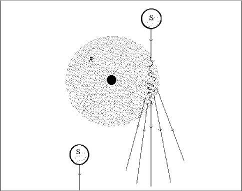
FIG. 1.: A black hole binary system with the stellar companion shown at two different positions in its orbit about the black hole. When the star is occulting as seen from the earth, electromagnetic radiation in the earth’s direction will be scattered by the tensor and scalar components of the gravitational field.

Asymptotically ($r\to\infty$) the major contribution to the electromagnetic wave field is given by

$$\phi_{2}^{(1,0)}\simeq C_{2}^{\pm}\,{e^{\pm i\,\bar{\omega}\,r}\over r}\equiv F_{2}^{\pm}\ ,$$ (46)

with a plus sign for ingoing modes and a minus sign for outgoing modes and $C_{2}^{\pm}=C_{2}^{\pm}(\theta)$ contains all the angular dependence in $\theta$. Therefore we can assume that $\phi_{0}^{(1,0)}=\phi_{1}^{(1,0)}\equiv 0$ (the so called phantom gauge, see Ref. [2]) in Eq. (45). This reduces the currents to

$$J_{1}^{(1,2)} = 0$$ (47)

$$J_{2}^{(1,2)} = -{a\over 2\,\sqrt{2}}\,\left({F_{2}^{*}\over\bar{\rho}^{*}}+{F_{2}\over\bar{\rho}}\right)\,\partial_{\theta}\phi$$ (48)

$$J_{3}^{(1,2)} = {a\over 2}\,F_{2}^{*}\,\partial_{r}\phi$$ (49)

$$J_{4}^{(1,2)} = i\,{K\over\Delta_{0}^{2}}\,F_{2}-{a\over 2}\,F_{2}\,\partial_{r}\phi\ ,$$ (50)

where

$$\phi\equiv\phi^{(0,2)}=-{a\over M}\,{r\over\rho^{2}}\ .$$ (51)

We can obtain an equation for $\phi_{2}^{(1,2)}$ alone from the third and fourth equations in Eq. (41). Upon defining as usual $W_{2}\equiv 2\,(\bar{\rho}^{*})^{2}\,\phi_{2}^{(1,2)}$ and $W_{1}\equiv\sqrt{2}\,\bar{\rho}^{*}\,\phi_{1}^{(1,2)}$ we obtain

$$\left({\cal D}_{0}-{1\over\bar{\rho}^{*}}\right)\,W_{2}-\left({\cal L}_{0}+{i\,\alpha\,\sin\theta\over\bar{\rho}^{*}}\right)\,W_{1}=2\,(\bar{\rho}^{*})^{2}\,F_{2}\,\left(i\,{K\over\Delta_{0}^{2}}-{a\over 2}\,\partial_{r}\phi\right)$$ (52)

$$\left({\cal L}_{1}^{\dagger}-{i\,\alpha\,\sin\theta\over\bar{\rho}^{*}}\right)\,W_{2}-\Delta_{0}\,\left({\cal D}_{0}^{\dagger}+{1\over\bar{\rho}^{*}}\right)\,W_{1}=-a\,\bar{\rho}^{*}\,(\bar{\rho}^{*}\,F_{2}+\bar{\rho}\,F_{2}^{*})\,\partial_{\theta}\phi\ .$$ (53)

Finally, upon using the commutation relation

$$\left[\Delta_{0}\,\left({\cal D}_{0}^{\dagger}+{1\over\bar{\rho}^{*}}\right),\left({\cal L}_{0}+{i\,\alpha\,\sin\theta\over\bar{\rho}^{*}}\right)\right]=0\ ,$$ (54)

one can eliminate $W_{1}$ and gets

$$\left[\Delta_{0}\,{\cal D}_{0}^{\dagger}\,{\cal D}_{0}+{\cal L}_{0}\,{\cal L}_{1}^{\dagger}+2\,i\,\bar{\omega}\bar{\rho}\right]\,W_{2}=T_{2}\ ,$$ (55)

where the source term is

$$T_{2} \equiv 2\,\Delta_{0}\,\left({\cal D}_{0}^{\dagger}+{1\over\bar{\rho}^{*}}\right)\,\left[(\bar{\rho}^{*})^{2}\,F_{2}\,\left(i\,{K\over\Delta_{0}^{2}}-{a\over 2}\,\partial_{r}\phi\right)\right]$$ (57)

$$-a\,\left({\cal L}_{0}+{i\,\alpha\,\sin\theta\over\bar{\rho}^{*}}\right)\,\left[\bar{\rho}^{*}\,(\bar{\rho}^{*}\,F_{2}+\bar{\rho}\,F_{2}^{*})\,\partial_{\theta}\phi\right]\ .$$

To leading order in $1/r$, the current is thus

$$T_{2}^{\pm}=2\,\bar{\omega}\,C_{2}^{\pm}\,(2\,M\,\bar{\omega}+i\,a^{2})\,\left\{\begin{array}[]{l}\,e^{+i\,\bar{\omega}\,r}\\ {r\over M}\,e^{-i\,\bar{\omega}\,r}\ .\end{array}\right.$$ (60)

In the expression above the contribution from the dilaton background is the one proportional to $a^{2}$, the remaining terms being purely KN. We can then write

$$T_{2}=T_{KN}+T_{a}\ ,$$ (61)

and separate the contributions for the two different sources. The L.H.S. of Eq. (55) can be expanded in powers of $1/r$ as well upon assuming

$$W_{2}\simeq A^{\pm}\,Z^{\pm}\,{e^{\pm i\,\bar{\omega}\,r}\over r^{n_{\pm}}}\ ,$$ (62)

where $Z^{\pm}=Z^{\pm}(\theta)$. One then finds

$$A^{\pm}\,Z^{\pm}\,{e^{\pm i\,\bar{\omega}\,r}\over r^{n_{\pm}-1}}\,2\,\bar{\omega}\,\left[2\,M\,\bar{\omega}+i\,(1\mp n_{\pm})\right]=T_{2}^{\pm}\ ,$$ (63)

from which it follows that $Z^{\pm}=C_{2}^{\pm}$,

$$\left\{\begin{array}[]{l}n_{+}=1\\ A^{+}_{KN}=1\\ A^{+}_{a}=i\,{a^{2}\over 2\,M\,\bar{\omega}}\ ,\end{array}\right.$$ (67)

and

$$\left\{\begin{array}[]{l}n_{-}=0\\ A^{-}_{KN}=2\,\bar{\omega}\,{2\,M\,\bar{\omega}-i\over 1+4\,M^{2}\,\bar{\omega}^{2}}\\ A^{-}_{a}={a^{2}\over M}\,{1+2\,i\,M\,\bar{\omega}\over 1+4\,M^{2}\,\bar{\omega}^{2}}\ .\end{array}\right.$$ (71)

We can conclude that the amplitudes of the electromagnetic waves scattered by the dilaton background become comparable to or greater than the intensity of the waves scattered by the KN background when $A_{a}^{-}\geq A_{KN}^{-}$, that is when (we restore the fundamental constants)

$$\bar{\omega}\leq\bar{\omega}_{c}\sim{a^{2}\,c^{3}\over G\,M}\ .$$ (72)

In string theory $a=1$ and $\bar{\omega}_{c}\sim 10^{35}$ Hz$/$kg. For example, for a solar mass black hole, the critical frequency would be about 100 kHz.

We observe that $\phi_{2}^{(1,2)}\sim 1/r^{2}$ is subleading with respect to $\phi_{2}^{(1,0)}\sim 1/r$. However, we can apply the same argument that we have formulated in [6], Section V, and conclude that the scattered waves $\phi_{2}^{(1,2)}$ are negligible with respect to free waves $\phi_{2}^{(1,0)}$ only when the scattering process occurs at large $r$, which is quite sensible, since strong effects from the dilaton background are not expected far away from the horizon. Therefore, adjusting the above mentioned argument to the present context, we claim that testable electromagnetic waves could be produced by the scattering of free Maxwell waves in a region (denoted by ${\cal R}$ in Fig. 1 and Ref. [6]) just outside the horizon where the gradient of the dilaton background is the strongest. Outside of ${\cal R}$ the scattered waves then propagate as free waves, thus one obtains

$$|\phi_{2}^{(1,2)}(r>r_{d})|\simeq|\phi_{2}^{(1,2)}(r_{d})|\,{r_{d}\over r}\ ,$$ (73)

where $r_{d}$ is the typical outer radial coordinate of the region ${\cal R}$.

The next step would now be to superpose a suitable selection of incoming modes $\phi_{2}^{(1,0)}$ to more realisitically model the electromagnetic radiation coming from the stellar companion of the black hole. Then, the corresponding superposition of excited modes $\phi_{2}^{(1,2)}$ would give us the scattered pattern and its time dependence due to the relative positions of the source and the black hole with respect to the observer. However, we feel that sensible results are out of reach of the analytical methods which are all we want to consider in the present work.

IV Geometrical optics effects

In the previous sections and in [6] we have studied the wave equations on the KND background. However, one might expect to obtain measurable effects on the propagation of light in such a background even at the level of geometrical optics [8].

To start with, we consider a simpler case, the (exact) RND solution [4],

$$ds^{2}=-e^{2\,\Phi}\,dt^{2}+e^{2\,\Lambda}\,dr^{2}+R^{2}\,\left(d\theta^{2}+\sin^{2}\theta\,d\varphi^{2}\right)\ ,$$ (74)

with

$$e^{2\,\Phi}=e^{-2\,\Lambda}=\left(1-{r_{+}\over r}\right)\,\left(1-{r_{-}\over r}\right)^{1-a^{2}\over 1+a^{2}}$$ (75)

$$R^{2}=r^{2}\,\left(1-{r_{-}\over r}\right)^{2\,a^{2}\over 1+a^{2}}$$ (76)

$$r_{+}=M\,\left[1+\sqrt{1-(1-a^{2})\,{Q^{2}\over M^{2}}}\;\right]$$ (77)

$$r_{-}=(1+a^{2})\,{Q^{2}\over M}\,\left[1+\sqrt{1-(1-a^{2})\,{Q^{2}\over M^{2}}}\;\right]^{-1}\ ,$$ (78)

and compute the deflection angle $\Delta\varphi_{1}$ of a null ray coming from infinity with an impact parameter $D_{1}=L_{1}/E_{1}\equiv D$ ($L_{1}$ is its angular momentum, $E_{1}$ its energy) and approaching the outer horizon $r_{+}$. Fromthe equations of motion for null geodesics one obtains an expression for $d\varphi/dr$ (see [2] for the details). On integrating the latter from $r=+\infty$ to $r_{1}$, the minimum radial position from the center of the hole reached by the ray, one finds

$$\Delta\varphi_{1}=2\,\left(\varphi(r_{1})-\varphi(\infty)\right)-\pi\ .$$ (79)

For the metric in Eq. (74) the above expression becomes

$$\Delta\varphi_{1}\simeq{2\,M\over r_{1}}\,\left[1+{4\,a^{2}-3\over 1+a^{2}}\,{Q^{2}\over 4\,M^{2}}\right]\ ,$$ (80)

where we have assumed $r_{+}\gg r_{-}$ and $Q/M\ll 1$. Eq. (80) already contains a dilatonic contribution and allows a comparison of the pure Reissner-Nordström case ($a=0$) with the Schwarzschild case ($Q=0$).

The radius $r_{1}$ is one of the zeros of $dr/d\varphi$ which in turn are the solutions of [2]

$$r_{1}^{3}-D_{1}^{2}\,(r_{1}-r_{+})=0\ .$$ (81)

Of course one requires $r_{1}>r_{+}$ for an unbound null ray that must escape to infinity.

Let us now consider a second fiducial null ray starting far away from the hole which lies in the same plane and points in the same direction as the first one but has a slightly different impact parameter $D_{2}=J_{2}/E_{2}=D+\delta$, where $\delta\ll D$. The two rays, rotated around the axis passing through the center of the hole and asymptotically parallel to both of them, define an annulus of which we just consider a small portion whose area is

$$A_{(-\infty)}\sim\Theta\,(D_{2}^{2}-D_{1}^{2})\simeq 2\,D\,\delta\,\Theta\ ,$$ (82)

where $\Theta$ is the relative angle between the two rays with respect to the axis passing through the center of the hole (we assume $\Theta$ to be small).

Each ray will then be deflected by the gravitational field of the hole according to Eq. (80). Since one has $r_{1}\not=r_{2}$, after having been scattered, the two fiducial rays will move at a relative angle

$$\Delta_{12}\equiv\Delta\varphi_{2}-\Delta\varphi_{1}=2\,M\,\left[1+{4\,a^{2}-3\over 1+a^{2}}\,{Q^{2}\over 4\,M^{2}}\right]\,\left({1\over r_{2}}-{1\over r_{1}}\right)\ .$$ (83)

Therefore the area that they define will change according to

$$A_{(r)}\sim r^{2}\,\Theta\,|\Delta_{12}|\ .$$ (84)

Although Eq. (81) is exactly soluable, the solutions are complicated, thus we will just consider the following approximations. Since we are interested in rays which travel close to the horizon, we assume $r_{i}=r_{+}+x_{i}$, with $x_{i}\ll r_{+}$ and, from Eq. (81) we get

$$D_{i}^{2}\simeq{r_{+}^{3}\over x_{i}}\gg r_{+}^{2}\ .$$ (85)

On solving the above equation for $x_{i}$ and substituting into Eq. (83) one finally obtains

$$\Delta_{12}\simeq{16\,M^{2}\,\delta\over D^{3}}\,\left[1+{2\,a^{4}+4\,a^{2}-5\over 1+a^{2}}\,{Q^{2}\over 8\,M^{2}}\right]\ ,$$ (86)

where the approximation $D_{i}\gg r_{+},\delta$ has been used, but $\delta\sim r_{+}$ is allowed.

The rate of decrease of the intensity $I$ can then be computed for any massless linear wave moving “between the two rays”,

$${I_{(r)}\over I_{(-\infty)}}={A_{(-\infty)}\over A_{(r)}}\sim{D^{4}\over M^{2}}\,\left[1-{2\,a^{4}+4\,a^{2}-5\over 1+a^{2}}\,{Q^{2}\over 8\,M^{2}}\right]\,{1\over r^{2}}\ .$$ (87)

The above result depends on the form of the metric only, and one might think of repeating the same computation for the KND case. However, as we pointed out in [6], up to the order at which we have computed it, the KND metric is just the KN metric. Therefore, no effect on the null rays can be expected from the dilaton background at any order below $Q^{4}/M^{4}$ when the black hole is rotating [9].

A final remark is due to clarify the difference between the approach shown in this section and the previous one. The solutions to the wave equation that we have found in section III display the full wave nature of the electromagnetic radiation and they also depend on the direct coupling between the dilaton field and the Maxwell field as formulated in the action (1). However, the results in the present section rely on the approximation of geometrical optics, thus neglecting the specific nature of the null rays which includes both the wave character and the coupling to the dilaton. Therefore it is not surprising that, in the geometrical optics picture no affect on the Maxwell rays is found for the KND geometry, while in the wave picture and at the same order of approximation in the charge-to-mass expansion the dilaton does affect electromagnetic waves.

By comparing the two approaches, one can conclude that the presence of a non-trivial background dilaton in KND (at the order included in our computation) affects only the intensity of the electromagnetic radiation and not its eikonal paths. This means that the calculation of gravitational lensing effects for comparison with measurements as tests for the existence of non-trivial dilaton fields must be carried to higher order in the expansion, and this can probably be done only numerically.

V Conclusions

We have shown that to the order at which we are working in perturbation theory the neglect of the gravitational and dilatonic waves with respect to the electromagnetic waves is internally consistent. This assumption has allowed us to obtain asymptotic expressions for ingoing and outgoing modes in the phantom gauge and the dilatonic contributions to these modes. Our analysis shows that electromagnetic waves scattered by the dilaton background have a critical frequency of approximately 0.1 MHz. This is in a frequency range which is not currently being studied by astrophysicists, because most stars emit relatively small amounts of energy in this range. On the other hand, if a detector were to be constructed to observe black hole binaries in this frequency range, the signal should be relatively clean, and any enhancement at this frequency in the intensity of the radiation from an occulting star would be a clear indication of the presence of a scalar component of gravity.

At any given frequency a decrease in the intensity of the radiation should be expected for an occulting star due to the scattering of the light by the gravitational field. However an exact expression for the intensity will have to wait until we are able to realistically model the electromagnetic radiation from the stellar companion of a black hole. This involves the superposition of the incoming Maxwell scalar modes, and this will probably entail a numerical investigation of the variation of the intensity of the star as a function of its orbital position.

In the geometrical approximation for a charged, non-rotating (Reissner-Nordström) dilaton black hole the integrated intensity decreases during occultation if $2\,a^{4}+4\,a^{2}-5>0$. In string theory $a=1$, and a decrease in the intensity of light from the occulting star as compared to its intensity when it eclipses the black hole would be evidence for a scalar component of gravity as predicted by string theory.

REFERENCES

• [1] R. Casadio, B. Harms, Y. Leblanc and P.H. Cox, Phys. Rev. D 55, 814 (1997).
• [2] S. Chandrasekhar, The mathematical theory of black holes, Oxford University Press, Oxford (1983).
• [3] V. Frolov, A. Zelnikov and U. Bleyer, Ann. Phys. (Leipzig) 44, 371 (1987).
• [4] G. W. Gibbons and K. Maeda, Nucl. Phys. B298, 741 (1988); G. T. Horowitz and A. Strominger, Nucl. Phys. B360, 197 (1991).
• [5] The fact that the addition of even a small amount of angular momentum drastically changes the qualitative features of the metric was already pointed out by J. H. Horne and G. T. Horowitz, Phys. Rev. D 46, 1340 (1992).
• [6] R. Casadio, B. Harms, Y. Leblanc and P.H. Cox, Phys. Rev. D 56, 4948 (1997).
• [7] Gravitational and electromagnetic waves do not decouple even in the KN background without the dilaton [2]. Of course here the situation is even more involved because there is one more field.
• [8] For the details of this approach see C.W. Misner, K.S. Thorne and J.A. Wheeler, Gravitation, Freeman, New York (1973), Chap. 25.6.
• [9] This conclusion seems to hold also for the metric in the so called string frame which is obtained from the one we have been using so far by a conformal transformation. Work in preparation.