Quantum Geometry and Black Holes

Abstract

Non-perturbative quantum general relativity provides a possible framework to analyze issues related to black hole thermodynamics from a fundamental perspective. A pedagogical account of the recent developments in this area is given. The emphasis is on the conceptual and structural issues rather than technical subtleties. The article is addressed to post-graduate students and beginning researchers.

I Introduction

In his Ph.D. thesis, Bekenstein suggested that, for a black hole in equilibrium, a multiple of its surface gravity should be identified with its temperature and a multiple of the area of its event horizon should be identified with its thermodynamic entropy [1]. In this reasoning, he had to use not only general relativity but also quantum mechanics. Indeed, without recourse to the Planck’s constant, $\hbar$, the identification is impossible because even the physical dimensions do not match. Around the same time, Bardeen, Carter and Hawking derived laws governing the mechanics of black holes within classical general relativity [2]. These laws have a remarkable similarity with the fundamental laws of thermodynamics. However, the derivation makes no reference to quantum mechanics at all and, within classical general relativity, a relation between the two seems quite implausible: since nothing can come out of black holes and since their interiors are completely inaccessible to outside observers, it would seem that, physically, they can only have zero temperature and infinite entropy. Therefore the similarity was at first thought to be purely mathematical. This viewpoint changed dramatically with Hawking’s discovery of black hole evaporation in the following year [3]. Using an external potential approximation, in which the gravitational field is treated classically but matter fields are treated quantum mechanically, Hawking argued that black holes are not black after all! They radiate as if they are black bodies with a temperature equal to $1/2\pi$ times the surface gravity. One can therefore regard the similarity between the laws of black hole mechanics and those of thermodynamics as reflecting physical reality and argue that the entropy of a black hole is given by $1/4$-th its area. Thus, Bekenstein’s insights turned out to be essentially correct (although the precise proportionality factors he had suggested were modified).

This flurry of activity in the early to mid seventies provided glimpses of a deep underlying structure. For, in this reasoning, not only do the three pillars of fundamental physics –quantum mechanics, statistical physics and general relativity– come together but coherence of the overall theory seems to require that they come together. It was at once recognized that black hole thermodynamics –as the unified picture came to be called– is a powerful hint for the quantum theory of quantum gravity, whose necessity was recognized already in the thirties.

Let us elaborate on this point. The logic of the above argument is as follows: Hawking’s calculations, based on semi-classical gravity, lead to a precise formula for the temperature which can then be combined with the laws of black hole mechanics, obtained entirely in the classical framework, to obtain an expression of the black hole entropy. Is there a more satisfactory treatment? Can one arrive at the expression of entropy from a more fundamental, statistical mechanical consideration, say by counting the number of ‘micro-states’ that underlie a large black hole? For other physical systems –such as a gas, a magnet, or the radiation field in a black body– to count the micro-states, one has to first identify the elementary building blocks that make up the system. For a gas, these are atoms; for a magnet, the electron spins; and, for radiation in a black body, the photons. What then are the analogous building blocks of a black hole? They can not be gravitons because the gravitational fields under consideration are static. Therefore, these elementary constituents must be essentially non-perturbative in nature. Thus, the challenges for candidate theories of quantum gravity are to: i) isolate these constituents; ii) show that the number of quantum states of these constituents which correspond to large black holes in equilibrium (for which the semi-classical results can be trusted) goes as the exponential of the area of the event horizon; iii) account for the Hawking radiation in terms of quantum processes involving these constituents and matter quanta; and, iv) derive the laws of black hole thermodynamics from quantum statistical mechanics.

These are difficult tasks because the very first step –isolating the relevant constituents– requires new conceptual as well as mathematical inputs. It is only recently, more than twenty years after the initial flurry of activity, that detailed proposals have emerged. One comes from string theory [4] where the relevant elementary constituents are certain objects (D-branes) of the non-perturbative sector of the theory. The purpose of this article is to summarize the situation in another approach, which emphasizes the quantum nature of geometry using non-perturbative techniques from the very beginning. Our elementary constituents are the quantum excitations of geometry itself and the Hawking process now corresponds to the conversion of the quanta of geometry to quanta of matter.

Although the two approaches are strikingly different from one another, they are also complementary. For example, as we will see, we will provide only an effective quantum description of black holes (in the sense that we first isolate the sector of the theory corresponding to isolated black holes and then quantize it). The stringy description, by contrast is intended to be fundamental. Also, in our approach, there is a one-parameter quantization ambiguity which has the effect that the entropy and the temperature are determined only up to a multiplicative constant which can not be fixed without an additional, semi-classical input. String theory, by contrast, provides the numerical coefficients unambiguously. On the other hand, so far, most of the detailed work in string theory has been focussed on extremal or near extremal black holes which are mathematically very interesting but astrophysically irrelevant. In particular, a direct, detailed treatment of the Schwarzschild black hole is not available. Our approach, by contrast, is not tied in any way to near-extremal situations and can in particular handle the Schwarzschild case easily. Finally, in the stringy approach, since most actual calculations –such as derivation of the Hawking radiation– are carried out in flat space, the relation to the curved black hole geometry is rather unclear. In our approach, one deals directly with the curved black hole geometry.

The article is organized as follows. Section 2 is devoted to preliminaries. We will first introduce the reader to basic properties of quantum geometry in non-perturbative quantum gravity and then briefly summarize a mathematical model called Chern-Simons theory which is needed in the description of the quantum geometry of the horizon. Main results are contained in section 3. We begin by describing the classical sector of the theory corresponding to black holes and then present the quantum description. By counting the relevant micro-states we are led to the expression of entropy. Finally, we indicate how Hawking evaporation can be regarded as a physical process in which the quanta of the horizon area are converted to quanta of matter. As suggested by the Editors, we shall try to communicate the main ideas at a level suitable for a beginning researcher who is not already familiar with the field. Therefore, the technicalities will be kept to a minimum; details can be found in [5, 6, 7, 8] and references cited therein.

II Preliminaries

A Quantum Theory of Geometry

In Newtonian physics and special relativity, space-time geometry is regarded as an inert and unchanging backdrop on which particles and fields evolve. This view underwent a dramatic revision in general relativity. Now, geometry encodes gravity thereby becoming a dynamical entity with physical degrees of freedom and Einstein’s equations tell us that it is on the same footing as matter. Now, the physics of this century has shown us that matter has constituents and the 3-dimensional objects we perceive as solids are in fact made of atoms. The continuum description of matter is an approximation which succeeds brilliantly in the macroscopic regime but fails hopelessly at the atomic scale. It is therefore natural to ask: Is the same true of geometry? Is the continuum picture of space-time only a ‘coarse-grained’ approximation which would break down at the Planck scale? Does geometry have constituents at this scale? If so, what are its atoms? Its elementary excitations? In other words, is geometry quantized?

To probe such issues, it is natural to look for hints in the procedures that have been successful in describing matter. Let us begin by asking what we mean by quantization of physical quantities. Take a simple example –the hydrogen atom. In this case, the answer is clear: while the basic observables –energy and angular momentum– take on a continuous range of values classically, in quantum mechanics their eigenvalues are discrete; they are quantized. So, we can ask if the same is true of geometry. Classical geometrical quantities such as lengths, areas and volumes can take on continuous values on the phase space of general relativity. Can one construct the corresponding quantum operators? If so, are their eigenvalues discrete? In this case, we would say that geometry is quantized and the precise eigenvalues and eigenvectors of geometric operators would reveal its detailed microscopic properties.

Thus, it is rather easy to pose the basic questions in a precise fashion. Indeed, they could have been formulated seventy years ago soon after the advent of quantum mechanics. To answer them, however, is not so easy. For, in all of quantum physics, we are accustomed to assuming that there is an underlying classical space-time. One now has to literally ‘step outside’ space-time and begin the analysis afresh. To investigate if geometrical observables have discrete eigenvalues, it is simply inappropriate to begin with a classical space-time, where the values are necessarily continuous, and then add quantum corrections to it. One has to adopt an essentially non-perturbative approach to quantum gravity. Put differently, to probe the nature of quantum geometry, one should not begin by assuming the validity of the continuum picture; the quantum theory itself has to tell us if the picture is adequate and, if it is not, lead us to the correct microscopic model of geometry.

Over the past decade, a non-perturbative approach has been developed to probe the nature of quantum geometry and to address issues related to the quantum dynamics of gravity. The strategy here is the opposite of that followed in perturbative treatments: Rather than starting with quantum matter on classical space-times, one first quantizes geometry and then incorporates matter. This procedure is motivated by two considerations. The first comes from general relativity in which some of the simplest and most interesting physical systems –black holes and gravitational waves– consist of ‘pure geometry’. The second comes from quantum field theory where the occurrence of ultraviolet divergences suggests that it may be physically incorrect to quantize matter assuming that space-time can be regarded as a smooth continuum at arbitrarily small scales.

The main ideas underlying this approach can be summarized as follows. One begins by reformulating general relativity as a dynamical theory of connections, rather than metrics [9]. This shift of view does not change the theory classically (although it suggests extensions of general relativity to situations in which the metric may become degenerate). However, it makes the kinematics of general relativity the same as that of $SU(2)$ Yang-Mills theory, thereby suggesting new non-perturbative routes to quantization. Specifically, as in gauge theories, the configuration variable of general relativity is now an $SU(2)$ connection $A^{i}_{a}$ on a spatial 3-manifold and the canonically conjugate momentum $E^{a}_{i}$ is analogous to the Yang-Mills ‘electric’ field. However, physically, we can now identify this electric field as a triad; it carries all the information about spatial geometry. In quantum theory, it is natural to use the gauge invariant Wilson loop functionals, ${\cal P}\,\exp\oint_{\alpha}\,A$, i.e., the path ordered exponentials of the connections around closed loops $\alpha$ as the basic objects [10, 11]. The resulting framework is often called ‘loop quantum gravity’.

In quantum theory, states are suitable functions of the configuration variables. In our case then, they should be suitable functions $\Psi(A)$ of connections. In field theories, the problem of defining ‘suitable’, i.e., of singling out normalizable states, is generally very difficult and involves intricate functional analysis. In our case, our space-time has no background metric (or any other field). This makes the problem more difficult because the standard methods from Minkowskian field theories can not be taken over. However, although it is surprising at first, it also makes the problem easier. For, the structures now have to be invariant under the entire diffeomorphism group –rather than just the Poincaré group– and, since the invariance group is so large, the available choices are greatly reduced. This advantage has been exploited very effectively by various authors to develop a new functional calculus on the space of connections. The integral calculus is then used to specify the (kinematical) Hilbert space of states and, differential calculus, to define physically interesting operators, including those corresponding to geometrical observables mentioned above.

For our purposes, the final results can be summarized as follows. Denote by $\gamma$ a graph in the 3-manifold under consideration with $E$ edges and $V$ vertices. (For readers familiar with lattice gauge theory, $\gamma$ can be regarded as a ‘floating’ lattice; ‘floating’ because it is not necessarily rectangular. Indeed, we don’t even know what ‘rectangular’ means because there is no background metric.) It turns out that the total Hilbert space ${\cal H}$ can be decomposed into orthogonal, finite dimensional subspaces ${\cal H}_{\gamma,{\vec{j}}}$, where ${\vec{j}}\equiv\{j_{1},\,...\,,j_{E}\}$ stands for an assignment of a non-zero half integer (‘spin’) –or, more precisely, a non-trivial irreducible representation of $SU(2)$– to each of the edges [12]. To specify a state in ${\cal H}_{\gamma,{\vec{j}}}$, one only has to fix an intertwiner at each vertex which maps the incoming representations at that vertex to the outgoing ones. (For a trivalent vertex, i.e., one at which precisely three edges meet, this amounts to specifying a Clebsch-Gordon coefficient associated with the $j$’s associated with the three edges.) Each resulting state is referred to as a spin network state [13]. The availability of this decomposition of ${\cal H}$ in to finite dimensional sub-spaces is a powerful technical simplification since it effectively reduces many calculations in quantum gravity to those involving simple spin systems.

Since the edges of a graph are one-dimensional, the resulting quantum geometry is polymer-like and, at the Planck scale, the continuum picture fails completely. It emerges only semi-classically. Recall that a polymer, although one dimensional at a fundamental level, exhibits properties of a three dimensional system when it is in a sufficiently close-knit state. Similarly, a state in which the fundamental one-dimensional excitations of quantum geometry are densely packed in a sufficiently complex configuration can approximate a three dimensional continuum geometry. Individual excitations are as far removed from a classical geometry as an individual photon is from a classical Maxwell field. Nonetheless, these elementary excitations do have a direct physical interpretation. Each edge carrying a label $j=\frac{1}{2}$ can be regarded as a flux line carrying an ‘elementary area’: In this state, each surface which intersects only the given edge of $\gamma$ has an area proportional to $\ell_{P}^{2}$, where $\ell_{P}$ is the Planck length. Thus, given a state in ${\cal H}_{\gamma,{\vec{j}}}$, quantum areas of surfaces are concentrated at points in which they intersect the edges of $\gamma$. Similarly, volumes of regions are concentrated at vertices of $\gamma$. The microscopic geometry is thus distributional in a precise sense.

In the classical theory, it is the triads that encode all the information about Riemannian geometry. The same is true in the quantum theory. The duals, $\Sigma^{i}_{ab}:=\epsilon_{abc}E^{c}_{i}$, of triads are 2-forms and one can show that, when smeared over two dimensional surfaces, the corresponding operators are well-defined and self-adjoint on the Hilbert space ${\cal H}$ [14]. Thus, in the technical jargon, triads are operator-valued distributions in two dimensions. Various geometric operators can be constructed rigorously by regularizing the appropriate functions of these triad operators [14, 15, 16, 17, 18]. Each is a self-adjoint operator and one can show that they all have purely discrete spectra. Thus, geometry is quantized in the same sense that energy and angular momentum are quantized in the hydrogen atom. Properties of these geometric operators have been studied extensively. However, for our purposes, it will suffice to focus only on certain properties of the area operators. We will conclude this section with a brief discussion of these properties.

The complete spectrum of the area operators is known. The minimum eigenvalue is of course zero. However, the value of the next eigenvalue –the ‘area-gap’– is non-trivial; it depends on the topology of the surface. Thus, it is interesting that quantum geometry ‘knows’ about topology. Although the spectrum is purely discrete, the eigenvalues $a_{S}$ crowd rather rapidly: for large eigenvalues $a_{S}$, the gap $\Delta a_{S}$ between $a_{S}$ and the next eigenvalue goes as $\Delta a_{S}\leq\exp(-\,\sqrt{a_{S}}/\ell_{P})$. It is because of this crowding that one can hope to reach the correct continuum limit. More precisely, the detailed behavior of the spectrum is important to recover the correct semi-classical physics. This may seem strange at first: Because the Planck length $\ell_{P}$ is so small, one might have thought that even if the spacing between area eigenvalues were uniform, say $\Delta a_{S}=\ell_{P}^{2}$, one would recover the correct semi-classical physics. Detailed analysis shows that is not the case. With an uniform level spacing, for example, one would not recover the Hawking spectrum even for a large black hole [19]. To obtain even a qualitative agreement with the semi-classical results it is necessary that the eigenvalues crowd and the specific exponential crowding one finds in this approach is also sufficient [14, 20]. Finally, let us describe the spectrum. For our purposes, it is sufficient to display only the eigenvalues that result when edges of a spin network state intersect the surface $S$ under consideration transversely. These are given by [14, 15, 21]:

$$A_{S}=8\pi\gamma\ell_{P}^{2}\sum_{p}\sqrt{j_{p}(j_{p}+1)},$$ (1)

where the sum is taken over all points $p$ where edges of a spin network state intersect $S$, $j_{p}$ are spin that label the intersecting edges, and $\gamma$ is an undetermined real number, known as the Immirzi parameter. Thus, the eigenvalues have an ambiguity of an overall multiplicative factor $\gamma$ which arises from an inherent quantization ambiguity in loop quantum gravity. As mentioned in the Introduction, to fix this ambiguity, one needs additional input, e.g., from semi-classical physics.

B Chern-Simons Theory

It turns out that our analysis of black hole thermodynamics will require, as a technical ingredient, certain results from a three-dimensional topological field theory known as the Chern-Simons theory. In this sub-section we shall recall these results very briefly.

In this theory, the only dynamical variable is a connection one-form $A$, which for our purposes can be assumed to take values in the Lie algebra of ${\rm SU}(2)$. The theory is ‘topological’ in the sense that it does not need or involve a background (or dynamical) metric. Fix an oriented three manifold $\Delta$ (which in our application will be a suitable portion of the black hole horizon), and consider connections $A$ on an ${\rm SU}(2)$ bundle over it. The action of the theory is given by:

$$S_{CS}={k\over 4\pi}\int_{\Delta}{\rm Tr}\left(A\wedge dA+{2\over 3}A\wedge A\wedge A\right).$$ (2)

where $\kappa$ is a coupling constant, also known as the ‘level’ of the theory, and the trace is taken in the fundamental representation of ${\rm SU}(2)$. The field equations obtained from the variation of this action simply say that the connection $A$ is flat on $\Delta$. Such connections can still be non-trivial if the manifold $\Delta$ has a non-trivial topology. An especially interesting case arises when $\Delta$ has a topology $S\times R$ where $S$ is a two-manifold with punctures, i.e., points removed. In this case, holonomies can be non-trivial around punctures; i.e., we can have a distributional non-trivial curvature which ‘resides at the deleted points’, even though on points included in $S$, the curvature vanishes everywhere. We will encounter this situation in the next section.

There are several ways to quantize Chern-Simons theory. For our purposes we will need some facts about its canonical quantization. Here, one has to first cast the theory into the Hamiltonian framework. This is achieved by carrying out the canonical (2+1) decomposition of the action, assuming that $\Delta$ has the topology of $S\times{\rm I}\!{\rm R}$, where $S$ is a two-dimensional manifold. The phase space consists only of the pullback of $A$ on $S$; unlike the Yang-Mills theory and general relativity, there are no ‘electric fields’. Thus, the components of the connection do not Poisson commute:

$$\left\{A_{a}^{i}(x),A_{b}^{j}(y)\right\}={4\pi\over k}\,{\varepsilon}_{ab}K^{ij}{\delta}^{2}(x-y).$$ (3)

where $K^{ij}$ is the Cartan-Killing metric on $su(2)$, and $\epsilon_{ab}$ is the (metric-independent) Levi-Civita density on $S$. As in all generally covariant theories, the Hamiltonian turns out to be a constraint

$$F_{ab}=0,$$ (4)

where $F_{ab}$ is the pull-back of the curvature of $A$ on $S$.

One is often interested in the quantization of this phase space in the situation in which the two-manifold $S$ has punctures. Then, as mentioned above, even though $F_{ab}$ vanishes on $S$, the holonomies around these punctures can be non-zero; intuitively, one can now regard the curvature as being ‘distributional, residing at the missing points’. To quantize the system, therefore, one has to provide certain additional information –quantum numbers– at these punctures. The resulting Hilbert space of states turns out to be finite dimensional, and the dimension depends on the quantum numbers labelling punctures. (See, e.g., [22].)

III Application to Black Holes

We are now ready to examine black hole thermodynamics from the fundamental perspective of non-perturbative quantum gravity. We will summarize the overall situation following a systematic approach developed in [5, 7, 8]. (For earlier work, see, e.g., [23].)

In general relativity, supergravity or indeed in any modern classical theory of gravity, using the causal structure one can define what one means by a black hole in full generality, without having to restrict oneself to any symmetries. With this notion at hand, one can then restrict attention to specific contexts, such as stationary or axi-symmetric situations. In quantum theory, the situation is not as satisfactory: in none of the approaches available today, does one have an unambiguous notion of a general, quantum black hole. Therefore, within each approach, a strategy is devised to circumvent this problem. The strategy of the present approach is the following: We will first pick out the sector of the classical theory that contains isolated black holes –the analogs of ‘equilibrium states’ in thermodynamics– and quantize that sector. This will provide an effective description. While this line of attack is sufficient for the analysis of black hole entropy and provides an avenue to understanding the Hawking radiation and laws of black hole mechanics from the perspective of quantum gravity, it is far from being fully satisfactory. For example, since we begin with a black hole sector of the classical theory, in a certain sense, the phase of the Hawking process in which the black hole has fully evaporated can not be encompassed in this approach. Consequently, as it stands, the approach is unsuitable for a comprehensive analysis of issues, such as ‘information loss’, related to the final stages of the evaporation process. The questions it is best suited to address are of the type: “Given that a space-time contains a black hole of a certain size, what is the associated statistical mechanical entropy and what is the spectrum of the Hawking radiation?” In a more fundamental approach, one would first construct the full theory of quantum gravity, single out, among solutions to the quantum field equations, those states which are to represent a quantum black hole, and analyze their physical properties.

So far, the detailed analysis exists only for non-rotating black holes possibly with electric and dilatonic charges. However, it is expected that the main features of the analysis will carry over also to the rotating case. For simplicity, in the main discussion, we will focus on uncharged black holes and comment on the charged case at the end.

A Phase space

To single out the appropriate sector of the theory representing isolated black holes, we will consider asymptotically flat space-times with an interior boundary (the horizon) on which the gravitational fields satisfy suitable boundary conditions. These conditions should be strong enough to capture the physical situation we have in mind but also weak enough to allow a large number of space-times. A detailed discussion of the appropriate boundary conditions can be found in [7]. Here, we will only present the underlying ideas.

FIG. 1.: Space-times of interest.

To motivate our choice of the boundary conditions, let us consider the space-time formed by a collapsing star (see Fig. 1). At some moment, the event horizon $\cal H$ forms. A part of the gravitational radiation emitted in the process falls in to the horizon along with the matter and the rest escapes to infinity. It is generally expected that the black hole would finally settle down. Just as in the calculation of entropy in thermodynamics one generally deals with systems that have reached equilibrium, here we will be primarily interested in the final phase in which the black hole has settled down. We will make an idealization and assume that after a certain retarded time no further matter or radiation falls in to the black hole –the black hole is isolated– and focus on the portion $\Delta$ of the event horizon to the future of this retarded time. Thus, in this region, the area of any two-sphere cross-section of the horizon will be constant, which we will denote by $A_{H}$.

Let us focus on the portion $\cal M$ of space-time, bounded by $\Delta$ and future null infinity ${\cal I}$, which can be regarded as the space-time associated with the isolated black hole under consideration. For simplicity, we will assume that the vacuum Einstein’s equations hold on $\cal M$, i.e. that all the matter has fallen in to the event horizon in the past of $\Delta$. Note that, as the figure shows, there could still be gravitational waves in ${\cal M}$ which escape to ${\cal I}$. It is these space-time regions $\cal M$ that constitute our sector of general relativity corresponding to isolated black holes.

This sector can be isolated technically by specifying boundary conditions which capture the intuitive picture spelled out above [5, 7]. It turns out, however, that, with our choice of boundary conditions at $\Delta$, the standard general relativity action in the connection variables is is no longer functionally differentiable: The variation of the action with respect to the connection contains a non-vanishing boundary term at $\Delta$. However, it turns out to be possible to add to the action a boundary term, whose variation exactly cancels the boundary term arising in the variation of ‘bulk’ action, thus making the total action differentiable. Furthermore, the boundary term turns out to be precisely the Chern-Simons action (2), where the coupling constant $k$ is now given by: $k=A_{H}/8\pi\gamma G$. It is quite surprising that there is such a nice interplay between general relativity, the boundary conditions for isolated black holes and the Chern-Simons theory.

To canonically quantize the resulting theory, one has to cast it first in the Hamiltonian form. This can be done in a standard fashion. As in the case without black holes [9], the basic canonical variables are the pull-backs $A_{a}^{i}$ of the gravitational connection to a spatial slice, such as $M$ in Fig. 1, and the triads $E^{a}_{i}$ on $M$. However, these fields are now required not only to be asymptotically flat but also to satisfy appropriate boundary conditions on the two-sphere boundary $S$ of $M$, i.e., the intersection of $M$ and ${\cal H}$, which are induced by our boundary conditions on space-time fields. First, the area of $S$ defined by the triads $E^{a}_{i}$ is a fixed constant, $A_{H}$. Second, the triads and the connections are intertwined by the relation

$$\underline{F}_{ab}^{i}=-\frac{2\pi\gamma}{A_{H}}\,\,\underline{\Sigma}_{ab}^{i}\,,$$ (5)

where, as before, $\Sigma_{ab}^{i}$ are the two-forms dual to the triads, $F_{ab}^{i}$ is the curvature of the connection $A_{a}^{i}$ on $M$ and where the under-bars denote pull-backs to the two-sphere boundary $S$ of $M$. Finally, the boundary conditions also imply that the pull-back of the connection $A_{a}^{i}$ to the boundary is reducible, i.e., the (based) holonomies of $A_{a}^{i}$ along closed loops within $S$ necessarily belong to an $U(1)$ sub-group of $SU(2)$. Although it is not necessary, for technical simplicity we can fix an internal vector field, $r^{i}$, on $S$ along which the curvature of the pulled-back connection is restricted to lie, and partially gauge fix the system. Then the gauge group on the boundary reduces from ${\rm SU}(2)$ to ${\rm U}(1)$. Furthermore, now only the $r$ component of (5) is nontrivial.

As one might expect, due to the addition of the surface term to the action, the fundamental Poisson brackets are modified; the symplectic structure also acquires a surface term. This new contribution is just the symplectic structure of the Chern-Simons theory on $\Delta$, where the coupling constant $k$ is now given by

$$k={A_{H}\over 8\pi\gamma G}.$$ (6)

Note that, up to a numerical coefficient, $k$ is simply the area of the horizon of black hole measured in the units of Planck area $\ell_{P}^{2}$.

The phase space consisting of the pairs $(A,E)$ satisfying our boundary conditions is infinite dimensional. It is clear, however, that not all the degrees of freedom described by fields $A,E$ are relevant to the problem of black hole entropy. In particular, there are ‘volume’ degrees of freedom in the theory corresponding to gravitational radiation propagating out to ${\cal I}$, which should not be taken into account as genuine black hole degrees of freedom. The ‘surface’ degrees of freedom describing the geometry of the horizon $S$ have a different status. It has often been argued that the degrees of freedom living on the horizon of black hole are those that account for its entropy. We take this viewpoint in our approach.

Note, however, that in the classical theory that we have described, the volume and surface degrees of freedom cannot be separated: all fields on $S$ are determined by fields in the interior of $M$ by continuity. Thus, strictly speaking, classically there are no independent surface degrees of freedom. However, as we described in subsection II A, in the quantum theory the fields describing geometry become distributional, and the fields on $S$ are no longer determined by fields in $M$; now there are independent degrees of freedom ‘living’ on the boundary. This striking difference arises precisely because distributional configurations dominate in non-perturbative treatments of field theories and would be lost in heuristic treatments that deal only with smooth fields. Furthermore, as we will see in the next sub-section, it is precisely these quantum mechanical surface degrees of freedom that account for the black hole entropy!

B Quantization and Entropy

To quantize the theory we proceed as follows. Since in the quantum theory the volume and surface degrees of freedom become independent, we can first quantize volume degrees of freedom by using the well-established techniques of loop quantum gravity summarized in section II A. We are interested only in those bulk states which endow the boundary $S$ with an area close to $A_{H}$. Boundary conditions (5) then imply that, for each such bulk state, only certain surface states are permissible. To calculate entropy, one then has, in essence, just to count the states satisfying these constraints.

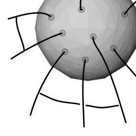
FIG. 2.: The flux lines of gravitational field pierce the black hole horizon and excite curvature degrees of freedom on the surface. These excitations are described by Chern-Simons theory and account for the black hole entropy in our approach.

More precisely, the situation is as follows. As discussed in subsection II A, in the bulk, we have a ‘polymer geometry’ with one dimensional excitations. That is, a typical state is associated with a graph $\gamma$ and the corresponding function $\Psi(A)$ of connections is sensitive only to what the connections do along the edges of $\gamma$. Let us take one such state and denote by $p_{1},\ldots,p_{n}$ the intersection points of the edges of $\gamma$ with the boundary $S$ (see Fig. 2). For such a state to be admissible as a micro-state of our large isolated black-hole –i.e., to belong to ‘the quantum micro-canonical ensemble’ underlying the classical black hole– two constraints have to be met at the boundary $S$: i) the quantum analog of the boundary condition (5) has to be satisfied; and, ii) the area assigned by the state to $S$ has to lie in the range $(A_{H}-\ell_{P}^{2},\,A_{H}+\ell_{P}^{2})$.

As indicated in section III A, only the $r$ component of (5) is non-trivial. Hence, in the quantum theory, our states have to satisfy

$$\left(\hat{\underline{F}}_{ab}^{i}r_{i}+\frac{2\pi\gamma}{A_{H}}\,\hat{\underline{\Sigma}}_{ab}^{i}r_{i}\right)\,\cdot\Psi=0.$$ (7)

Let us first consider $\underline{\hat{\Sigma}}$, the dual of the triad operator. As indicated in section II A, this operator is distributional and, on the boundary $S$, the result of its action turns out to be concentrated precisely at the points $p_{1},\ldots,p_{n}$ where the edges of $\gamma$ intersect $S$. Hence, the boundary condition (7) implies that in the quantum theory the state $\Psi$ has a non-trivial dependence only on those connections $\underline{A}$ on $S$ which are flat everywhere except the points $p_{1},\ldots,p_{n}$, where its curvature is distributional. Recall that the Poisson brackets between the connections $\underline{A}$ are precisely those of the Chern-Simons theory. Thus the ‘surface part’ of the state is precisely a Chern-Simons quantum state associated with the two sphere $S$ with punctures $p_{1},\ldots,p_{n}$. To summarize, the ‘volume part’ of the state encodes a polymer-type geometry in the bulk, while the surface part is a Chern-Simons state, the two being ‘locked together’ by (7).

Let us now turn to the second constraint on the states, namely the requirement on area assigned to $S$ by these states. To count the number of states satisfying this constraint, let us examine the eigenstates of the area operator which intersect $S$, as above, in $n$ points $p_{1},\ldots,p_{n}$. These are precisely the spin network states introduced in section II A. Therefore, each intersection point $p$ now inherits a spin label $j_{p}$ from the edge that intersects $S$ in $p$. For notational simplicity, from now on, we will refer to the pair $(p,j_{p})$ as a puncture and often denote it simply by $j_{p}$. The area constraint tells us that we should restrict our attention to the sets ${\cal P}$ of punctures,

$${\cal P}=\{j_{p_{1}},\ldots,j_{p_{n}}\}$$

for which the area eigenvalue (associated to $S$ by the corresponding spin-network state)

$$a_{\cal P}=8\pi\gamma\ell_{P}^{2}\sum_{p}\,\sqrt{j_{p}(j_{p}+1)}$$

lies in the interval $A_{H}-\ell_{P}^{2}\leq a_{\cal P}\leq A_{H}+\ell_{P}^{2}$. We will refer to these ${\cal P}$ as the permissible sets of punctures.

Now, each set ${\cal P}$ of punctures gives rise to a Hilbert space of Chern-Simons quantum states of the connection on $S$. Denote it by ${\cal H}_{\cal P}$. These are the surface states which are ‘compatible’ with the given permissible set ${\cal P}$ of punctures. Now, it follows from standard results in Chern-Simons theory that, for a large number of punctures, the dimension of ${\cal H}_{\cal P}$, goes as

$${\rm dim}{\cal H}_{\cal P}\sim\prod_{j_{p}\in{\cal P}}(2j_{p}+1),$$ (8)

Intuitively it is obvious that to calculate the entropy it suffices to add up these dimensions, i.e. that the entropy $S_{\rm bh}$ is simply

$$S_{\rm bh}=\ln\,\,\sum_{\cal P}{\rm dim}\,(H_{\cal P})$$ (9)

where the sum extends over permissible sets of punctures. It is rather straightforward to calculate the sum for large $A_{H}$, and we have:

$$S_{\rm bh}=\frac{\gamma_{0}}{4\ell_{P}^{2}\gamma}\,A_{H},\quad{\rm where}\quad\gamma_{0}=\frac{\ln{2}}{\pi\sqrt{3}}.$$ (10)

(The appearance of $\gamma$ can be traced back directly to the formula for the eigenvalues of the area operator, (1)). Thus, in the limit of large area, the entropy is proportional to the area of the horizon. If we fix the quantization ambiguity by setting the value of the Immirzi parameter $\gamma$ to the numerical constant $\gamma_{0}$ (which is of the order of $1$), then the statistical mechanical entropy is given precisely by the Bekenstein-Hawking formula.

Are there independent checks on this preferred value of $\gamma$? The answer is in the affirmative. One can carry out this calculation for Reissner-Nordstrom as well as dilatonic black holes. A priori it could have happened that, to obtain the Bekenstein-Hawking value, one would have to re-adjust the Immirzi parameter for each value of the electric or dilatonic charge. This does not happen. The entropy is still given by (10) and hence by the Bekenstein-Hawking value when $\gamma=\gamma_{0}$. The way in which the details work out shows that this is quite a non-trivial check.

We conclude with two remarks.

1. An intuitive way to think about the quantum states that underlie an isolated black hole is as follows. As indicated in section II A, the edges of spin networks can be thought of as flux lines carrying area. These flux lines endow the horizon $S$ with its area and also pin it (see Fig. 2), exciting the curvature degrees of freedom at the punctures via (7). With each given configuration of flux lines, there is a finite dimensional Hilbert space ${\cal H}_{\cal P}$ describing the quantum states associated with these curvature excitations. Heuristically, one can picture the horizon $S$ as a pinned balloon and regard these surface degrees of freedom as describing the ‘oscillatory modes’ compatible with the pinning.

2. A detailed calculation of the black hole entropy shows that the states that dominate the counting correspond to punctures all of which have labels $j=1/2$. For, in this configuration, the number of punctures needed to approximate a given $A_{H}$ is the largest. One can thus visualize each micro-state as providing a yes-no decision or ‘an elementary bit’ of information. It is very striking that this picture coincides with the one advocated by John Wheeler in his “It from Bits” scenario [24]. Thus, in a certain sense, our analysis can be regarded as concrete, detailed realization of those qualitative ideas.

C Black Hole Radiance

Since the number of micro-states of a large black hole grows as the exponential of its area in Planck units, a quantum black hole is system with an astonishingly large number of micro-states. Hence, the statistical mechanical approximations one normally makes, e.g., in treating the emission spectra in atomic physics, are satisfied here very easily. Over twenty years ago, therefore, Bekenstein [25] used analogies from atomic physics to develop a strategy for analyzing black hole radiance from microscopic considerations. Most of the current work in this area uses this strategy in one form or another. Our approach follows this trend.

The mechanism responsible for the radiance in our approach is based on the following qualitative picture. Consider the micro-states of a large black hole introduced in section III B, and let the black hole be initially in an eigenstate ${|\Gamma\rangle}$ of the horizon area operator. Radiation is emitted when the black hole jumps to a nearby state ${|\Gamma^{\prime}\rangle}$ with a slightly smaller area. This change in area corresponds to a change $\Delta M_{\Gamma\Gamma^{\prime}}$ in the mass of the black-hole which gets radiated away. Suppose, for simplicity, that the emitted particle is of rest mass zero. Then, the frequency $\omega_{\Gamma\Gamma^{\prime}}$ of the particle when it reaches infinity is given by $\Delta M_{\Gamma\Gamma^{\prime}}=\hbar\omega_{\Gamma\Gamma^{\prime}}$. Since the area spectrum (1) is purely discrete, the black-hole spectrum is also discrete at a fundamental level: the emission lines occur at specific discrete frequencies. At first one might worry [19] that such a spectrum would be very different from the continuous, black-body spectrum derived by Hawking using semi-classical considerations. However, as indicated in section II A, because the level spacing between the eigenvalues of the area operator decreases exponentially for large areas, the separation between the spectral lines can be so small that the spectrum can be well-approximated by a continuous profile [20, 14].

To determine the intensities of spectral lines and hence the form of the emission spectrum, as in atomic physics, we can use Fermi’s golden rule. Thus, the probability of a transition $\Gamma\to\Gamma^{\prime}$ with the emission of a quantum of radiation is given by

$$W_{\Gamma\to\Gamma^{\prime}}={2\pi\over\hbar}\,|V_{\Gamma\Gamma^{\prime}}|^{2}\,\delta(\omega-\omega_{\Gamma\Gamma^{\prime}}){\omega^{2}d\omega d\Omega\over(2\pi\hbar)^{3}},$$ (11)

where $V_{\Gamma\Gamma^{\prime}}$ is the matrix element of the part of the Hamiltonian of the system that is responsible for the transition, $d\Omega$ is the element of the solid angle in the direction in which the quantum is emitted, and $\omega_{\Gamma\Gamma^{\prime}}$ is the frequency of the quantum. (For brevity, we have suppressed the dependence of this matrix element on initial and final states of the quantum field describing the radiation.) The total energy $dI$ emitted by the system per unit time in transitions of this particular type can be obtained simply by multiplying this probability by $\hbar\omega$ times the probability ${\rm Pr}(\Gamma)$ to find the system in the initial state ${|\Gamma\rangle}$:

$$dI(\Gamma\to\Gamma^{\prime})=2\pi\omega\,\,{\rm Pr}(\Gamma)\,\,|V_{\Gamma\Gamma^{\prime}}|^{2}\,\delta(\omega-\omega_{\Gamma\Gamma^{\prime}}){\omega^{2}d\omega d\Omega\over(2\pi\hbar)^{3}}$$ (12)

The question for us is: For quantum black holes, how do these intensity distributions compare with those of a black-body? To answer the question, one has to calculate the probability distribution ${\rm Pr}(\Gamma)$ of the black hole, and the matrix elements $|V_{\Gamma\Gamma^{\prime}}|$ of the Hamiltonian responsible for transitions. Recall, however, that, in atomic physics, the general form of the spectrum is usually determined by the probability distribution of initial states and by such qualitative aspects of the underlying dynamics as selection rules for quantum transitions. The detailed knowledge of the matrix elements is needed only to determine the finer details of the spectrum. The situation for quantum black holes is analogous.

The overall picture can be summarized as follows. For a large black hole, since the typical energies of the emitted particles are negligible compared to the black hole mass, it is reasonable to appeal to basic principles of equilibrium statistical mechanics and conclude that all accessible micro-states occur with equal probability. Now, the entropy $S$ goes as the logarithm of the number of states. Hence, the probability for occurrence of any one permissible micro-state ${|\Gamma\rangle}$ is $\exp(-S)$. General considerations involving Einstein’s A and B coefficients now imply that the mean number $n_{\omega lm}$ of quanta of frequency $\omega$ and angular momentum quantum numbers $l,m$ emitted by the black hole per unit time is given by

$$n_{\omega lm}={\sigma_{\omega lm}\over e^{\hbar\omega/T}-1},$$ (13)

where, $T$ is the thermodynamic temperature,

$${1\over T}:={dS\over dM}$$ (14)

and $\sigma_{\omega lm}$ is the absorption cross-section of the black hole in the mode $\omega lm$. (See, e.g., [25, 6]).

Although we have phrased the argument in terms of black holes –the system now under consideration– most of the reasoning used so far is quite general. In the case of the black-hole, we know further that the entropy $S$ is given by $A_{H}/4$, which fixes the thermodynamic temperature in terms of the parameters of the black hole. This turns out to be precisely the temperature that Hawking was led to associate, in the external potential approximation, with the spontaneously emitted radiation. Recall that the initial semi-classical reasoning had an unsatisfactory feature: the Hawking temperature is the property of the emission spectrum at infinity and it is not a priori clear that it is related to the thermodynamic properties of the black hole. The reasoning given above, based on the micro-states of the quantum black hole itself, fills this gap; the temperature in the emission spectrum is indeed the statistical mechanical temperature of the black hole.

Finally, we can obtain the intensity spectrum. Since the s-waves dominate in the emission from non-rotating black holes, we can focus only on the $l=0$ modes. Then, to obtain the intensity spectrum, one has to multiply $n_{\omega,l=0}$ by the energy $\hbar\omega$ and the density of states $\omega^{2}d\omega d\Omega$ in the mode, and integrate out the angular dependence. The result is:

$$I(\omega)d\omega\sim{\hbar\omega^{3}\sigma_{\omega}\,d\omega\over e^{\hbar\omega/T-1}};$$ (15)

Thus, very general arguments lead us to the result that the emission spectrum of the black hole is thermal, in the sense that it has the form (15). The problem now reduces to that of calculating the absorption cross-section $\sigma_{\omega}$ from first principles. Since the Hawking analysis is semi-classical, there it was consistent to use the classical value of this cross-section. In full theory, on the other hand, we need to compute it quantum mechanically. Thus, the remaining question is: Does the cross-section calculated in the full quantum theory agree with the classical result? If so, one would have a derivation of Hawking radiation from fundamental considerations.

Now, in the classical theory, the cross-section $\sigma_{\omega}$ in (15) is an approximately constant function of $\omega$ (equal to the horizon area $A_{H}$). In our quantum treatment, on the other hand, there is an obvious potential problem. To see this, recall first from section III B that the most likely micro-states are the ones in which each puncture is labelled by $j=\frac{1}{2}$. Indeed they dominate the distribution in the sense that they already provide the leading order contribution to the entropy. Hence, one would expect that, transitions $j=0\to j=\frac{1}{2}$ would completely dominate the absorption cross-section. In this case, $\sigma_{\omega}$ would be peaked extremely sharply at a single frequency and the final spectrum (15) would therefore look very different from Hawking’s. However, this transition is simply forbidden by a selection rule! More precisely, if the interaction Hamiltonian responsible for the transitions is gauge invariant –which it must be, on general physical grounds– its matrix element between the initial and final states of the above type is identically zero. The situation here is again analogous to that in atomic physics where the selection rules are obtained simply by examining the transformation properties of the interaction Hamiltonian under the rotation group.

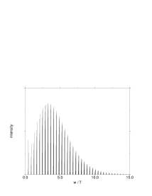
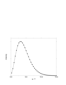
FIG. 3.: Emission lines with their intensities (above) and the total intensity of the radiation emitted per frequency interval as a function of frequency (below).

With this obstruction out of the way, one can proceed with the calculation of the quantum absorption cross-section. Now one can argue that, for a large class of Hamiltonians, the quantum absorption cross-section is close to the classical one [6]. For instance, if for allowed transitions the dependence on $\Gamma$ and $\Gamma^{\prime}$ of $V_{\Gamma,\Gamma^{\prime}}$ is negligible, the intensity spectrum is given by FIG 3. In the first plot, the intensities of lines are computed using (11). (Here, the overall multiplicative factors are neglected; hence there are no units on the $y$ axis.) The second plot is obtained by first dividing the frequency range into small intervals and then adding the intensities of all the lines belonging to the same interval. It brings out the fact that, although the emission occurs only at certain discrete frequencies, the enveloping curve of the spectrum is thermal.

IV Discussion

The key ideas underlying our approach can be summarized as follows. In the spirit of equilibrium statistical mechanics, we consider large, isolated black holes (in four space-time dimensions). When appropriate boundary conditions at the horizon are imposed, we find that the bulk action of Einstein’s theory has to be supplemented by a surface term at the horizon which is precisely the Chern-Simons action. We then quantize the resulting sector of the theory. As one might expect from the general structure of quantum field theories, the fields describing geometry become distributional in the quantum theory. Furthermore, our background independent functional calculus tells us that the fundamental quantum excitations are of a specific type: they are one-dimensional, like polymers. The horizon acquires its area from the points where these one-dimensional excitations pierce it transversely. Associated with each bulk state which endows the horizon with a given area, there are ‘compatible’ surface states on the horizon itself which come from the quantization of Chern-Simons theory thereon. The total number of these ‘compatible’ Chern-Simons states grows exponentially with the area, whence the entropy is proportional to the area of the horizon. Finally, using Fermi’s golden rule, one can compute the probabilities for transitions among these horizon states. Transitions that decrease the area are accompanied by an emission of particles. From rather general considerations, one can conclude that the emission spectrum is thermal, in agreement with Hawking’s semi-classical calculations.

At its core, this is a rather simple and attractive picture of quantum black holes. However, it is far from being complete and further work is being carried out in a number of directions. First, as in other approaches, the calculations leading to the Hawking spectrum are based on a number of simplifying assumptions. Although by and large these are physically motivated, it is important to make sure that the final results are largely insensitive to them. Second, all the detailed work to date has been carried out only for non-rotating black holes. Although the underlying ideas are robust, considerable technical work will be required to extend the results to the non-rotating case. Third, the role played by field equations in this program is yet to be fully understood. Since the construction of the phase space and the associated symplectic structure is delicate, it is clear that, as it stands, the framework is closely tied to general relativity; extension to higher derivative theories, for example, will probably involve significant modifications. (Extension to supergravity, by contrast, may not.) Furthermore, in the quantum analysis, the ‘kinematic part’ of quantum Einstein’s equations –the so called Gauss and diffeomorphism constraints– play a significant role. However, the role of the Hamiltonian constraint is rather limited and needs to be better understood. Finally, attempts to derive the laws of black hole mechanics in full the quantum theory have just begun.

Perhaps the most puzzling and unsatisfactory aspect of the framework is that there is an inherent quantization ambiguity which leads to a one-parameter family of unitarily inequivalent theories. It shows up in various technical expressions through the Immirzi parameter $\gamma$; while the classical theory is completely insensitive to the value of $\gamma$, the quantum theory is not. Roughly, this parameter is analogous to the $\theta$ angle in Yang-Mills theory and as such its value can be fixed only experimentally. Black hole evaporation can be taken to be an appropriate experiment for this purpose. Now, it is reasonable to assume that Hawking’s semi-classical analysis [3] would agree with the experimental result for a large black hole. Hawking’s answer is recovered in our approach only when the Immirzi parameter is fixed to be $\gamma_{0}=\ln 2/\pi\sqrt{3}$. That is, it appears that, only for this value of $\gamma$ would the non-perturbative quantum theory, with all its polymer geometries and quantized areas, agree, in semi-classical regimes, with the standard quantum field theory calculation in curved space-times. However, the issue is far from being settled. Perhaps a new viewpoint will emerge and it may well cause the present picture to change in certain respects. However, the picture does have a striking coherence. Indeed, it is remarkable that results from three quite different areas –classical general relativity, quantum geometry and the Chern-Simons theory– fit together without a mismatch to provide a consistent and detailed description of the micro-states of black holes. At several points in the analysis, the matching is delicate and consistency could easily have failed. Since that does not happen, it seems reasonable to expect that the lines of thought summarized here will continue to serve as main ingredients also in the final picture.

V Acknowledgements

Much of this review is based on joint work with John Baez and Alejandro Corichi. We are grateful to them and to the participants of the 1997 quantum gravity workshop at the Erwin Schrödinger Institute for many stimulating discussions. We are especially grateful to John Baez for comments on early versions of the manuscipt. The authors were supported in part by the NSF grants PHY95-14240, INT97-22514 and by the Eberly research funds of Penn State. In addition, KK was supported by the Braddock fellowship of Penn State.

REFERENCES

- [1] J. D. Bekenstein, Black holes and entropy, Phys. Rev. D7, 2333-2346 (1973). J. D. Bekenstein, Generalized second law of thermodynamics in black hole physics, Phys. Rev. D9 3292-3300 (1974).
- [2] J. W. Bardeen, B. Carter and S. W. Hawking, The four laws of black hole mechanics, Commun. Math. Phys. 31, 161-170 (1973).
- [3] S. W. Hawking, Particle creation by black holes, Commun. Math. Phys. 43, 199-220 (1975).
- [4] A. Strominger and C. Vafa, Microscopic origin of the Bekenstein-Hawking entropy, Phys. Lett. B379, 99-104 (1996). J. Maldacena and A. Strominger, Statistical entropy of four-dimensional extremal black holes, Phys. Rev. Lett. 77 428-429 (1996).
- [5] A. Ashtekar, J. Baez, A. Corichi, K. Krasnov, Quantum geometry and black hole entropy, Phys. Rev. Lett. 80, No. 5, 904-907 (1998).
- [6] K. Krasnov, Quantum geometry and thermal radiation form black Holes, gr-qc/9710006.
- [7] A. Ashtekar, A. Corichi, K. Krasnov, Black hole sector of the gravitational phase space (CGPG Pre-print, 1998).
- [8] A. Ashtekar, J. Baez, K. Krasnov, Quantum geometry of black hole horizons (CGPG Pre-print, 1998).
- [9] A. Ashtekar, New variables for classical and quantum gravity, Phys. Rev. Lett. 57, 2244-2247 (1986). A. Ashtekar, New hamiltonian formulation of general relativity, Phys. Rev. D36, 1587-1602 (1987).
- [10] T. Jacobson and L. Smolin, Non-perturbative quantum geometries, Nucl. Phys. B299, 295 (1988).
- [11] C. Rovelli and L. Smolin, Loop space representation of quantum general relativity, Nucl. Phys. B331, 80 (1990).
- [12] J. Baez, Spin networks in non-perturbative quantum gravity, in “The Interface of Knots and Physics”, edited by L. Kauffman, American Mathematical Society, Providence, 1996, pp. 167-203.
- [13] C. Rovelli and L. Smolin, Spin networks and quantum gravity, Phys. Rev. D52, 5743-5759 (1995).
- [14] A. Ashtekar and J. Lewandowski, Quantum theory of geometry I: Area operators, Class. Quant. Grav. 14, A55-A81 (1997).
- [15] C. Rovelli and L. Smolin, Discreteness of area and volume in quantum gravity, Nucl. Phys. B442, 593 (1995); Erratum: Nucl. Phys. B456, 734 (1995).
- [16] A. Ashtekar and J. Lewandowski, Quantum theory of geometry II: Volume Operators, Adv. Theo. Math. Phys. 1, 388-429 (1997).
- [17] T. Thiemann, A length operator for canonical quantum gravity, gr-qc/9606092.
- [18] R. Loll, Spectrum of the volume operator in quantum gravity, Nucl. Phys. B460 143-154 (1996).
- [19] J. Bekenstein, V. Mukhanov, Spectroscopy of the quantum black hole, Phys. Lett. B360, 7 (1995).
- [20] M. Barreira, M. Carfora, C. Rovelli, Physics with non-perturbative quantum gravity: radiation from a quantum black hole, Gen. Rel. and Grav. 28, 1293-1299 (1996).
- [21] K. Krasnov, On the constant that fixes the area spectrum in canonical quantum gravity, Class. Quant. Grav. 15, L1-L4 (1998).
- [22] R. K. Kaul and P. Majumdar, Quantum black hole entropy, gr-qc/9801080.
- [23] C. Rovelli, Black hole entropy from loop quantum gravity, Phys. Rev. Lett. 14 3288-3291 (1996). C. Rovelli, Loop quantum gravity and black hole physics, Helv. Phys. Acta. 69 582-611 (1996). K. Krasnov, Geometrical entropy from loop quantum gravity, Phys. Rev. D55 3505-3513 (1997). K. Krasnov, On statistical mechanics of Schwarzschild black holes, Gen. Rel. and Grav. 30, No. 1, 53-68 (1998).
- [24] J. Wheeler, It from bits and quantum gravity, in “Sakharov Memorial Lectures on Physics”, edited by L. Keldysh and V. Feinberg, Nova Science, New York, 1992, Vol. 2.
- [25] J. D. Bekenstein and A. Meisels, Einstein A and B coefficients for a black hole, Phys. Rev. D15, 2775-2781 (1977).