Abstract

In the coming decade, the LIGO/VIRGO network of ground-based kilometer-scale laser interferometer gravitational wave detectors will open up a new Astronomical window on the Universe: gravitational waves in the frequency band $10$ to $10^{4}$ Hz. In addition, if the proposed, 5 million kilometer long, space based interferometer LISA flies, another window will be opened in the frequency band $10^{-4}$ to $1$ Hz. We review the various possible sources that might be detected in these frequency bands, and the information that might be obtainable from observed sources. Several key possible sources are inspirals and coalescences of neutron-star neutron-star and/or neutron-star black-hole binaries; inspirals, mergers, and ringdowns of black-hole black-hole binaries (both solar mass and supermassive); stellar core collapse; rapidly rotating neutron stars; the formation of supermassive black holes; and inspirals of compact objects into supermassive black holes.

1 Introduction

This review of gravitational wave sources is divided into three sections. First, we review the detector sensitivities that have been achieved to date and discuss projected sensitivities for detectors now under construction. Second, we summarize the current observational upper limits on gravitational waves in various frequency bands.

The main body of this review will consist of a survey of various anticipated sources of waves. Each anticipated source can be roughly characterized by a characteristic frequency $f$ and a characteristic value of strain amplitude $h$. However, it is important to also note that sources vary widely with respect to how uncertain is the rate of their occurrence in the Universe. The enterprise of anticipating potential gravitational wave sources is extremely uncertain. For most sources that we can conceive of, either the wave strengths are uncertain by several orders of magnitude, or the event rate is uncertain by several orders of magnitude, or the very existence of the source itself is very uncertain. While there are some important exceptions such as coalescing compact binaries, these are the exception rather than the rule. The upside of this great uncertainty is the potential for gravitational wave astronomy to bring us new and interesting information.

For more details on the topics discussed here, the reader is encouraged to consult the detailed recent review articles by Thorne [1, 2, 3, 4], and also the review article by Allen [5] on stochastic gravitational waves.

2 Detector Sensitivities: Achieved and Projected

As is well known, there are two technologies which are being pursued for detection of gravitational waves. The first is to monitor the modes of vibration of a solid test mass which is cooled to very low temperatures. Such detectors are called resonant mass detectors, or more colloquially “bars”. The second technology is to monitor the relative displacement of suspended test masses using laser interferometry.

There are presently operating several cylindrical resonant mass antennae: the ALLEGRO detector at Louisiana State University [6], the NIOBE detector at the University of Perth, Australia [7], the EXPLORER detector at the University of Rome [8]. All of these detectors are operating at temperatures of a few degrees Kelvin and have sensitivities of order $h\sim{\rm(several)\ }\times 10^{-19}$. There are also one or two so-called third generation detectors which are operating at temperatures of a few tens of miliKelvin: the AURIGA detector at the University of Legarno, Italy [9], and the NAUTILUS detector at the University of Rome [10]. These detectors have sensitivities of order $h\sim{\rm(several)\ }\times 10^{-20}$ [10].

In addition, there are plans to construct a new generation of resonant mass detectors which will be spherical, or nearly spherical (TIGAs or Truncated Icosahedral Gravitational Arrays [12]), or hollow spheres. Detectors in the planning stage include the GRAIL project in the Netherlands [13], the OMNI-1 project in Brazil, and the TIGA project in the USA [12]. These detectors have design sensitivities of order $10^{-21}$; see Fig. 1 below. Attaining this sensitivity level will require reducing the so-called noise temperature by several orders of magnitude, and so will not be an easy task. More details on resonant mass detectors can be found in the contribution by Massimo Cerdonio to this proceedings.

Interferometer detectors have several advantages over resonant mass detectors, the primary one being that they are intrinsically broadband while resonant detectors are narrowband. The technology for such detectors has been continuously under development for several decades. Today an international network of kilometer-scale, interferometer detectors is under construction, consisting of:

• The American LIGO project [11], which initially will consist of three separate interferometers, an interferometer with $4\,{\rm km}$ arms in Livingston, Louisiana, and two interferometers with armlengths of $2\,{\rm km}$ and $4\,{\rm km}$ in Hanford, Washington. The detectors will come online around 2001.

• The French-Italian VIRGO project [14], which is constructing an interferometer with $3\,{\rm km}$ arms near Pisa, Italy. This detector is also planned to come online around 2001.

• The British-German GEO600 project [15], which is constructing a $600$ meter long interferometer near Hanover, Germany, coming online around the year 2000.

• The Japanese TAMA project [16], which is constructing a $300$ meter interferometer near Tokyo.

There are also several prototype interferometers, for instance, the LIGO 40m prototype and the Garching and Glasgow interferometers associated with the GEO 600 project. The kilometer-scale interferometers will act as a coordinated network: for each burst of waves, the data from all the detectors will be analyzed to obtain the two independent waveforms $h_{+}(t)$ and $h_{\times}(t)$, and also the direction to the source. More details on this network can be found in the contribution by Norna Robertson to these proceedings.

Both resonant mass detectors and earth-based interferometer detectors are limited to the frequency band $10\,{\rm Hz}\mathrel{\raise 1.29167pt\hbox{$<$}\mkern-14.0mu\lower 2.58334pt\hbox{$\sim$}}f\mathrel{\raise 1.29167pt\hbox{$<$}\mkern-14.0mu\lower 2.58334pt\hbox{$\sim$}}10^{4}\,{\rm Hz}$. At lower frequencies, the background of time varying near-zone Newtonian gravitational fields produced by objects on the Earths surface (winds in the atmosphere, seismic waves in the Earth’s crust etc.) becomes very large. In order to attempt to measure gravitational waves in the band of frequencies $10^{-4}\,{\rm Hz}\mathrel{\raise 1.29167pt\hbox{$<$}\mkern-14.0mu\lower 2.58334pt\hbox{$\sim$}}f\mathrel{\raise 1.29167pt\hbox{$<$}\mkern-14.0mu\lower 2.58334pt\hbox{$\sim$}}1\,{\rm Hz}$, it is necessary to go into space. Laser interferometry can be used to monitor the distances between spacecraft and thus to measure gravitational waves. One proposed mission of this kind is the Laser Interferometer Space Antenna (LISA), which the European Space Agency tentatively plans to fly around 2015 [17]. LISA consists of six spacecraft in a triangular configuration in a solar orbit.

Figure 1 shows the noise levels that have been achieved to date in several representative detectors: bar detectors in 1976, in 1990 (Louisiana/Rome), in 1997, and the Caltech 40 meter prototype interferometer in 1990 and 1994. Also shown in Fig. 1 are the projected noise levels for future detectors: the first generation “initial” LIGO interferometers, later “advanced” LIGO interferometers, the LISA interferometer, and proposed TIGA resonant mass detectors. There will also be a generation of interferometers in LIGO intermediate between the initial interferometers and the advanced interferometers; these “enhanced interferometers” will be obtained by incrementally improving the various elements of the initial interferometers over a time scale of a few years. In Fig. 2 we compare the noise spectra for all the major interferometer projects.

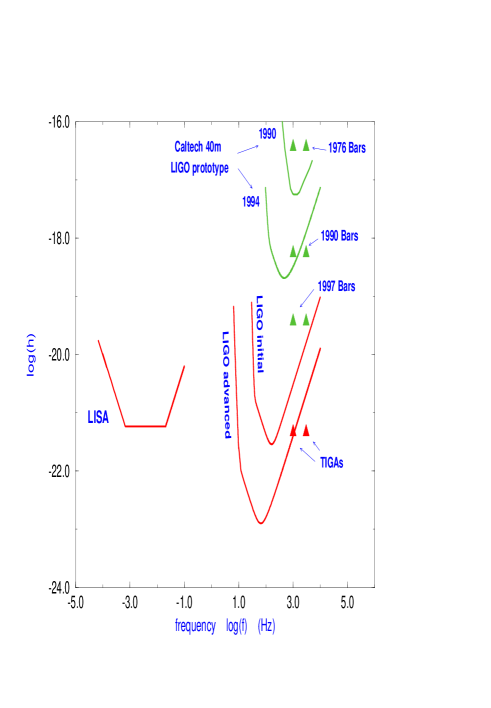
Figure 1.  : This plot shows the noise levels that have been achieved to date in several gravitational wave detector systems: the Caltech 40m interferometer [18], and the best bar detectors in 1976, [1], in the early 1990’s [2], and in 1997 [10]. It also shows that projected noise levels for future detector systems: initial and advanced LIGO interferometers [11], the spacebased LISA interferometer [2], and future generations of resonant mass detectors in the form of truncated icosahedral gravitational arrays (TIGAs) [20]. For the broadband interferometer detectors the quantity plotted is $h_{\rm rms}(f)\equiv\sqrt{fS_{h}(f)}$. For the narrowband resonant mass detectors (bars and TIGAs), the quantity plotted is $h_{\rm rms,bar}\equiv\alpha h_{\rm rms}(f_{0})\sqrt{f_{0}/\Delta f}$, where $\Delta f$ is the bandwidth of the noise spectrum, $f_{0}$ is the central frequency, and $\alpha$ is a constant of order unity chosen so that narrowband and broadband detectors will have the same value of $h$ on this plot if they are equally efficient at detecting broadband, burst waves [21].

For the broadband, interferometer detectors, the quantity plotted in Figs. 1 and 2 is the the rms dimensionless strain per unit logarithmic frequency, $h_{\rm rms}(f)$. This is defined so that the total noise-induced fluctuation in the output $h(t)$ of any detector can be written as

$$\langle h(t)^{2}\rangle=\int_{-\infty}^{\infty}\,d(\ln f)\ h_{\rm rms}(f)^{2}.$$ (1)

For the resonant mass detectors, on the other hand, the quantity $1/h_{\rm rms}(f)$ sharply peaked, and the signal-to-noise ratio for any broadband burst of waves is proportional to $\int df1/h_{\rm rms}(f)^{2}=\Delta f/h_{\rm rms}(f_{0})^{2}$, where $\Delta f$ is the bandwidth and $f_{0}$ is the central frequency. In Fig. 1 we plot for resonant mass detectors the quantity

$$h_{\rm rms,bar}\equiv\alpha\,\sqrt{f_{0}\over\Delta f}\,h_{\rm rms}(f_{0}),$$ (2)

where $\alpha$ is a constant of order unity chosen so that narrowband and broadband detectors will have the same value of $h$ if they are equally efficient at detecting broadband, burst waves [21]. [Note that, when considering the detection of periodic signals, one should instead compare directly the values of $h_{\rm rms}(f)$ of bars and interferometers.]

For a given broadband burst of waves, broadband detectors can measure the gravitational waveform $h(t)$, whereas narrowband detectors can essentially measure only the Fourier transform of the waveform at the resonant frequency. Although we have treated the planned TIGA/spherical detectors as narrowband instruments above, in fact they will have $\Delta f/f_{0}\sim 0.1$ [12], in contrast to bar detectors to date which have $\Delta f/f_{0}\sim 10^{-3}$. A “xylophone” of TIGAs could thus act as a broadband instrument [12].

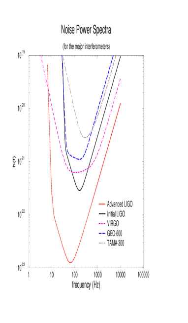
Figure 2.  : The projected noise spectra for the current major interferometer projects. The LIGO spectra were taken from Fig.10 of Ref. [11] and the spectra for the other interferometers were obtained from Ref. [22].

Consider now how strong waves have to be in order to be detected. There are three different types of gravitational waves: burst waves, periodic waves and stochastic waves. For each type of wave, let $h_{\rm amp}(t)$ denote the physical size of the metric perturbation. For burst waves, a signal with characteristic frequency $f_{c}$ will be detectable whenever $h_{\rm eff}\mathrel{\raise 1.29167pt\hbox{$>$}\mkern-14.0mu\lower 2.58334pt\hbox{$\sim$}}h_{\rm rms}(f_{c})$, where the effective strain amplitude $h_{\rm eff}$ is

$$h_{\rm eff}=h_{\rm amp}{\sqrt{{\cal N}_{\rm cycles}}\over\sqrt{2\ln\left[T/\Delta t\right]}}.$$ (3)

Here ${\cal N}_{\rm cycles}$ is the number of cycles of the waveform in the bandwidth of the detector, $T$ is the total duration of the data set in which one searches for a signal, and $\Delta t$ is the effective sampling time [23]. For periodic waves, a signal with frequency $f_{c}$ will be detectable when $h_{\rm eff}\mathrel{\raise 1.29167pt\hbox{$>$}\mkern-14.0mu\lower 2.58334pt\hbox{$\sim$}}h_{\rm rms}(f_{c})$, where

$$h_{\rm eff}=h_{\rm amp}{\sqrt{T\Delta f}\over\sqrt{2\ln\left[T\Delta f\right]}}$$ (4)

and $\Delta f$ is the range of frequencies one searches through. Finally, stochastic waves will be approximately detectable when $h_{\rm eff}\mathrel{\raise 1.29167pt\hbox{$>$}\mkern-14.0mu\lower 2.58334pt\hbox{$\sim$}}h_{\rm rms}$, where

$$h_{\rm eff}=h_{\rm amp}\sqrt{T\Delta f}$$ (5)

and $\Delta f$ is the bandwidth over which the detector is sensitive. Plotting $h_{\rm eff}$ versus $h_{\rm rms}$ for several different detectors and various different sources of waves illustrates the waves’ detectability. The definitions (3) – (5) are approximate but correct to within factors of order unity; more precise characterizations of detectability for burst, periodic and stochastic waves can be found in Refs. [1], [70] and [5], respectively.

3 Indirect detections and observational upper limits

The most celebrated indirect detection of gravitational waves is of course the monitoring of the orbital decay of the binary pulsar PSR 1913+16, for which the decay rate agrees with the prediction of general relativity to better than $1\,\%$ [24]. Aside from this, several different techniques have been used to place upper limits on the energy density in gravitational waves in different frequency bands. One technique is to monitoring the radio signals from interplanetary spacecraft; such signals would be Doppler shifted in a characteristic way by a burst of gravitational waves. The limits obtained from this technique [1] are illustrated in Fig. 3. Another technique is to monitor precisely the arrival times of radio pulses from pulsars (accuracy $\sim 1\,\mu{\rm s}$) over several years; the resulting limits [25] are shown in Fig. 3. From primordial nucleosynthesis we obtain the constraint on primordial gravitational waves that $\int d\ln f\,\Omega_{g}(f)\mathrel{\raise 1.29167pt\hbox{$<$}\mkern-14.0mu\lower 2.58334pt\hbox{$\sim$}}10^{-5}$ [5]; this limit does not apply to waves that were produced after neucleosynthesis. Finally, it is likely that some portion of the anisotropy of the cosmic microwave background radiation is due to primordial gravitational waves (the remaining portion being due to density or scalar perturbations). The current observations of the anisotropy spectrum cannot distinguish between scalar and gravitational wave contributions. Thus, these observations provide upper bounds on $\Omega_{g}(f)$ at low frequencies as illustrated in Fig. 3 [5]. They may also constitute an indirect detection of gravitational waves, although current theoretical prejudice suggests that the gravitational wave contribution to the anisotropy is smaller than the noise level in the observations to date.

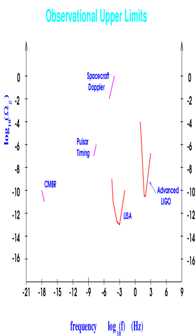
Figure 3.  : Current observational upper limits on gravitational wave energy density in various frequency bands, together with the projected sensitivities of advanced LIGO interferometers and of LISA.

The limits in Fig. 3 are shown in terms of the quantity $\Omega_{g}(f)$, which is the energy density in gravitational waves per unit logarithmic frequency divided by the critical energy density $\rho_{\rm critical}$ necessary to close the Universe:

$${\Omega_{g}(f)} \equiv {1\over\rho_{\rm critical}}\,{dE\over d\ln f\,d^{3}x}(f)$$

$$= \left({f\over 100\,{\rm Hz}}\right)^{2}\,\left({h_{\rm amp}\over 1.3\times 10^{-20}}\right)^{2}\,\left({100{\rm km}\,{\rm s}^{-1}\,{\rm Mpc}^{-1}\over H_{0}}\right)^{-2},$$

where $H_{0}$ is the Hubble constant.

4 Overview of Sources

As discussed above, the the high frequency band of $10\,{\rm Hz}\mathrel{\raise 1.29167pt\hbox{$<$}\mkern-14.0mu\lower 2.58334pt\hbox{$\sim$}}f\mathrel{\raise 1.29167pt\hbox{$<$}\mkern-14.0mu\lower 2.58334pt\hbox{$\sim$}}10^{4}\,{\rm Hz}$ is the domain of earth-based instruments. Key sources in this band are stellar core collapses, coalescences of compact binaries (neutron star – neutron star, neutron star – black hole, and black hole – black hole binaries), vibrating/precessing neutron stars, and black hole births. The low frequency band of $10^{-4}\,{\rm Hz}\mathrel{\raise 1.29167pt\hbox{$<$}\mkern-14.0mu\lower 2.58334pt\hbox{$\sim$}}f\mathrel{\raise 1.29167pt\hbox{$<$}\mkern-14.0mu\lower 2.58334pt\hbox{$\sim$}}10^{-1}\,{\rm Hz}$ is the domain of LISA. Here the sources are binary stars, formation and coalescences of supermassive black holes (SMBHs), and capture of compact objects by SMBHs. Sources of stochastic waves include parametric amplification of vacuum fluctuations during inflation; defects such as cosmic strings, and phase transitions in the early Universe. These sources can produce waves over a huge frequency band from $f\sim 10^{-18}\,{\rm Hz}$ to $f\sim{\rm MHz}$. In addition, the superposition of very many indistinguishable coalescing compact binary signals or stellar core collapse signals may produce a detectable stochastic background in the high frequency band [26]. Finally, more speculative sources include theoretical constructs such as naked singularities, boson stars, soliton stars, etc.

5 Stellar Core Collapse

Type II supernovae occur roughly once every 40 years in our Galaxy. The rate of stellar core collapses could be somewhat larger than this, since some stellar core collapses could be electromagnetically quiet and/or associated with the accretion induced collapse of white dwarfs. While the electromagnetic signal is dominated by the ejected mantle, the gravitational wave signal is dominated by the dynamics of the collapsing core. Numerical modeling of the dynamics of core collapse and bounce is complex: despite much work in this area there is not yet a firm consensus. The amount and characteristics of the gravitational wave emission depends on hydrodynamic processes that have not yet been well modeled, and also on the initial rotation rate of the degenerate stellar core before collapse, which is poorly known. Thus, there are large uncertainties associated with this type of source. In fact, our knowledge is so poor that the event detection rate could be as large as many per year with initial LIGO interferometers, or as poor as less than one per year with advanced LIGO interferometers.

There is a critical value of the initial angular momentum $J$ of the degenerate stellar core. If $J=0$, then the core will bounce once nuclear densities are reached at $r\sim 10\ {\rm km}$, where $r$ is the radius. Otherwise the eccentricity $e$ increases during the collapse; to a good approximation

$${T\over W}\sim e^{2}\sim{J^{2}\over GM^{3}}\,{1\over r},$$ (7)

where $T$ is the rotational kinetic energy of the core, $W$ is its gravitational potential energy, $J$ is its conserved angular momentum, and $M$ is its mass. The bounce occurs at eccentricities of order unity when

$$J\sim J_{\rm crit}\sim\sqrt{{GM^{3}\over 10\,{\rm km}}},$$

which corresponds to initial rotation periods of a few seconds. For $J\gg J_{\rm crit}$, centrifugal flattening will hangup the collapse. On the other hand, if $J\ll J_{\rm crit}$, there is no centrifugal hangup and it is thought that core remains axisymmetric during the collapse. Numerical simulations predict that in this case the total energy radiated from the collapse and bounce is $\Delta E_{\rm rad}\sim 10^{-7}M_{\odot}c^{2}$, and the effective strain amplitude is [27]

$$h_{\rm eff}\sim 3\times 10^{-22}\left({30\,kpc\over r}\right).$$

Such a core collapse would be visible only in the local group of galaxies by LIGO/VIRGO/GEO.

Consider now the case in which $J\gg J_{\rm crit}$. Here centrifugal flattening and hangup occur before nuclear densities are reached; the protoneutron star could form a disc with radius $\sim 100\,{\rm km}$ or larger. If $T/W\mathrel{\raise 1.29167pt\hbox{$>$}\mkern-14.0mu\lower 2.58334pt\hbox{$\sim$}}0.3$, theory suggests that a the fluid configuration is unstable to becoming non-axisymmetric via a dynamical triaxial instability. This would greatly enhance the gravitational wave emission; a purely axisymmetric body can emit waves only via its collapsing motion, whereas a non-axisymmetric body can emit waves via its rotational motion. Such a triaxial instability has been seen in numerical simulations [28], in which the hydrodynamical processes are treated in a simple and approximate way. [Note however that one recent numerical simulation [29] finds that the non-axisymmetry does not appreciably enhance the gravitational wave emission contrary to expectations.] If such an instability occurs, as much as $\sim 10^{-3}M_{\odot}c^{2}$ of energy could be radiated into gravitational waves, and such collapses could be seen out to the VIRGO cluster by initial LIGO interferometers and to several hundred Mpc by advanced LIGO interferometers. However, the fraction of core collapses (if any) which become very non-axisymmetric is unknown. Nevertheless, even if only one core collapse in $10^{4}$ undergoes a tri-axial instability, such collapses might be the most common type of core collapse seen by the detectors. Several specific scenarios for non-axisymmetry are reviewed by Thorne [4].

There is little observational evidence concerning the initial rotation rates of degenerate stellar cores. Two points are worth noting, however. First, the increasing evidence that neutron stars undergo substantial kicks in supernovae [30] (achieving velocities $\mathrel{\raise 1.29167pt\hbox{$>$}\mkern-14.0mu\lower 2.58334pt\hbox{$\sim$}}1500\,{\rm km}{\rm s}^{-1}$ in some cases) suggests that core collapses are very non-symmetric. Second, observations suggest that newborn neutron stars are typically not born spinning near the breakup angular velocity that one would expect if the core collapse has an excess of angular momentum [31]. The traditional view has been that this indicates that most pre-collapse stellar cores are slowly rotating. However, it has recently been predicted that newborn neutron stars can spin down from near maximal rotation down to $\sim 20\ {\rm Hz}$ within a year or so due to $r$-mode instabilities (see Sec. 7 below). Thus, there need not be a contradiction between the observational evidence that rapidly spinning (periods $\sim$ milliseconds) neutron stars have typically accreted most of their angular momentum, and the supposition that most pre-collapse degenerate stellar cores could be rapidly rotating.

Detecting stellar core collapses would have several payoffs for astronomy [1]. If the core collapse were close enough to produce a detectable flux of neutrinos, one could constrain neutrino masses by comparing the arrival times of gravitational waves and neutrinos. For example, a coincident detection of gravitational waves and neutrinos from the supernova SN1987a would have yielded the limit $m_{\nu}\mathrel{\raise 1.29167pt\hbox{$<$}\mkern-14.0mu\lower 2.58334pt\hbox{$\sim$}}4\,{\rm eV}$. One could also obtain information from the gravitational waveforms about the dynamics of the core collapse and bounce, tipoff optical astronomers before optical supernova first brighten (so they can measure the early portion of the light curve), and obtain observational evidence about the rate of formation of neutron stars.

6 Coalescences of Compact Binaries

6.1 Neutron star – Neutron star coalescences

The most reliable source for the LIGO/VIRGO/GEO network is the coalescences of neutron star/neutron star (NS/NS) binaries; this type of source has been studied theoretically in great detail over the last several years. The event rate is fairly well understood from observations of progenitor NS/NS systems in our own Galaxy: the distance to which one must look to see 3 events per year has been estimated to be $\sim 200\,{\rm Mpc}$ [32, 33]. [Recent revisions to the pulsar distance scale indicate that this distance could be somewhat larger, perhaps $\sim 400\,{\rm Mpc}$ [34]]. The range of initial LIGO interferometers for NS/NS binaries is $\sim 25\,{\rm Mpc}$, while that of the enhanced interferometers will be $\sim 250\,{\rm Mpc}$. There is a clean separation in the gravitational waveforms between an inspiral phase of the signal, which carries most of the detection signal-to-noise ratio and which is fairly well understood theoretically, and a subsequent merger phase, which depends on the internal structure of the stars and which is poorly understood theoretically [35]. Fortunately, understanding the details of the merger phase is not necessary for detecting the signals; for detection one will use the inspiral waves.

Detection of gravitational waves from NS/NS binaries would test the fairly popular theory that NS/NS mergers are the source of gamma ray bursts, which are seen at a rate of roughly once per day by satellite gamma ray detectors, and whose origin has been a longstanding puzzle. The rate of burst detections of a few per day is roughly consistent with the inferred rate of NS/NS mergers out to cosmological distances, and amount of energy supplied by a NS/NS merger is (marginally) sufficient to produce the observed $\gamma$ ray energy fluxes for a source at a cosmological distance. In the last year new evidence has been uncovered that gamma ray bursts are cosmological in origin rather than Galactic, which favors the NS/NS coalescence hypothesis: optical counterparts of some particular bursts have been seen at cosmological distances [36]. On the other hand, while the light curves and spectra of the bursts seem to be well fit by a model of an expanding relativistic fireball, there are theoretical difficulties in understanding how NS/NS mergers (or NS/BH or BH/BH mergers) could give rise to such fireballs with sufficiently low baryon contamination. [Too many baryons in the fireball would convert too much of the fireball’s energy into kinetic energy of the baryons instead of into radiation].

During the inspiral of the two stars, general relativistic effects are large as the orbital velocity is about $\sim 20\%$ of the speed of light at the point where most of the detection signal-to-noise ratio is obtained. The signal is very clean however: to a very good approximation, the two stars can be treated as point masses with intrinsic spins. The gravitational waveform is then determined by the relativistic gravitational interaction between the two point masses; all of the other complicated physical effects that occur (heating and tidal distortion of the stars, interactions involving the stars’ magnetic fields etc.) have a negligible effect on the gravitational waveforms in the inspiral phase [37].

This cleanliness means that the characteristics of the waveforms can be predicted in advance, and that the technique of matched filtering [1] can be used to detect the waves. By cross-correlating the outputs of the various interferometers in the network with theoretical template waveforms, one can both detect the waves and also measure the binaries parameters: masses, spins, orbital elements, sky location, distance etc. Very high accuracy templates are not required to detect the waves: currently available, post-2-Newtonian templates will be adequate in most cases [38]. By contrast, in order to extract the parameters of the binary with acceptably small systematic errors, very high accuracy templates will be required; such templates are under construction [39]. It is possible that approximate post-Newtonian waveforms may be substantially improved using the method of Padé approximants [40]. Much theoretical work has been done on how accurately the parameters of the binary can be measured; however, the parameter-extraction accuracies are currently only known to within factors of order 2.

There are several payoffs of measuring the inspiral waves from coalescing binaries. One will be able to experimentally measure for the first time various non-linear aspects of general relativity such as gravitational wave tails [41, 42] and possibly in some cases the dragging of inertial frames [43]. It will be possible to constrain non general-relativistic theories of gravity, for example one will be able to improve on solar system bounds on the dimensionless parameter $\omega$ of Brans-Dicke theory [44], and one will obtain constraints on the “graviton mass” [45]. One could identify the sources of gamma ray bursts by comparing their arrival times to those of gravitational wave bursts. If the event rate is large enough, one will be able to accumulate statistics on the distances, approximate sky locations, and masses of many ($\sim 100$) coalescences. This information will directly probe the distribution of Galaxies on scales $400\,{\rm Mpc}\mathrel{\raise 1.29167pt\hbox{$<$}\mkern-14.0mu\lower 2.58334pt\hbox{$\sim$}}D\mathrel{\raise 1.29167pt\hbox{$<$}\mkern-14.0mu\lower 2.58334pt\hbox{$\sim$}}4\,{\rm Gpc}$ with a resolution of $\sim 200\,{\rm Mpc}$ [41]; the distribution of Galaxies on such large scales has not yet been probed in redshift surveys. In addition, one will be able to attempt to measure the three cosmological parameters: the Hubble constant, the cosmological constant, and the closure parameter $\Omega$. Monte Carlo simulations suggest that with one year’s observations with advanced LIGO interferometers, one will be able to measure the Hubble constant to $\sim\,1\%$ and the other two parameters with fractional accuracies of a few tens of percent [46]. [Of course, it is likely that these parameters will already have been accurately measured by the time advanced interferometer sensitivity levels are achieved, by the MAP and PLANCK satellite measurements of the CMBR [47]].

Turn, now, to the gravitational waves from the merger stage of coalescing binaries. These will carry information about the internal structure of the neutron stars and potentially about the equation of state of nuclear matter at high densities. Efforts are underway to understand the dynamics of the merger process and the features of the emitted waves using numerical simulations. So far, simulations of the merger have been limited to the Newtonian or post-1-Newtonian approximations [48]. There are indications that it might be necessary to simulate the merger numerically in full general relativity; efforts are underway in this direction. The merger waveforms will have most of their power at high frequencies of several hundred Hz or higher. Unfortunately, broadband laser interferometers have poor performance at these high frequencies (see Fig. 1 above). However, it might be possible to measure the merger waves with specialized narrowband interferometers which are designed to have enhanced sensitivity near some chosen frequency and worsened sensitivities elsewhere [49], or with the next generation of resonant mass antennae (TIGAs or spheres).

6.2 NS/BH and BH/BH binaries

The other types of coalescing compact binary that might be measured are NS/BH and BH/BH binaries, as illustrated in Fig. 4. For the NS/BH case the signal can be divided into inspiral and merger phases as before; for the BH/BH case the signal can be divided into three phases, inspiral, merger and ringdown [50].

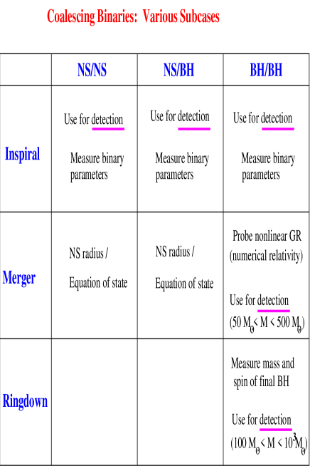
Figure 4.  : A summary of the various phases of the waves (inspiral, merger, and ringdown) for the three different types of coalescing binary, and the usefulness of each phase for each type of source.

There are several fundamental differences between the NS/BH and BH/BH cases, and the NS/NS case:

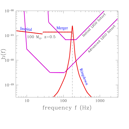
Figure 5.  : A plot of the wave strength $\sqrt{5}h_{\rm eff}$ for waves from a binary black hole coalescence of total mass $100M_{\odot}$ at redshift $z=1$, together with the noise levels $\sqrt{5}h_{\rm rms}$ for initial and advanced LIGO interferometers (adapted from Ref. [50]). The energy spectra for the merger waves and the ringdown waves are taken from the crude models of Ref. [50] ($10\%$ of total mass energy radiated in merger waves and $3\%$ in ringdown waves). Notice that the inspiral waves are not visible with the initial LIGO interferometers, and barely visible with the advanced. For this type of source, it will be necessary to try to detect the waves using the merger or ringdown waves directly.

First, the event rates for NS/BH and BH/BH coalescences are far less certain than NS/NS coalescences, since so far we have no observed progenitor systems. Arguments based on progenitor evolution scenarios suggest an event rate rate very roughly $\sim 3\,{\rm yr}^{-1}$ within $200\,{\rm Mpc}$, i.e., the same rate as for NS/NS binaries, in both the NB/BH and BH/BH cases [32]. [A recent estimate by Brown and Bethe reduces this distance to $100\,{\rm Mpc}$ for the NS/BH case [51]]. There are three classes of BH/BH binaries: field binaries, binaries formed by capture processes in galactic centers, and capture binaries in globular clusters. Siggurdson and Hernquist have argued that there is generically at least one BH/BH event per core collapse globular cluster [52]; this yields $\sim 3$ BH/BH events per year within a distance of $600\,{\rm Mpc}$ using the extrapolation method of Sec. 3.1 of Ref. [32]. For field BH/BH binaries, recent estimates of the coalescence rate by experts in binary evolution theory range from $\sim 10^{-8}\,{\rm yr}^{-1}$ to $\sim 10^{-6}\,{\rm yr}^{-1}$ in our Galaxy [53, 54], to completely negligible [55]. There are large uncertainties associated with these theoretical estimates of the coalescence rates.

Second, for BH/BH coalescences, the merger waves will bring information about the dynamics of general relativity in a highly dynamical, highly nonlinear, highly non-spherical regime that has never before been probed experimentally. A major effort is underway in the numerical relativity community to simulate the mergers of black holes, driven in part by the possibility of performing comparisons with gravitational wave data; see the article by Ed Seidel in this proceedings. The overall energy and the amount of information carried by the merger waves are still very uncertain.

Third, the inspiral waves are stronger for NS/BH and BH/BH sources than for NS/NS sources, simply because of their greater mass. The initial LIGO interferometers can reach to $\sim 40\,{\rm Mpc}$ for a BH/BH binary of total mass $M=5\,M_{\odot}$ and to $\sim 300\,{\rm Mpc}$ for $M=50M_{\odot}$ [50]; enhanced interferometers can see roughly ten times further and advanced interferometers about 30 times further. Thus, BH/BH coalescences might be detected early by the LIGO/VIRGO network, and may be seen before NS/NS coalescences. Note also that if BH/BH events are seen, the most commonly detected events will be the largest mass systems, since the increase in signal-to-noise ratio with increasing mass very likely more than compensates for the decrease in the mass function with increasing mass [56].

Fourth, the frequency at which the inpiral ends, i.e., at which the spinning-point-mass approximation fails, decreases as the total mass of the system is increased. For sufficiently massive systems, the regime of optimum sensitivity for LIGO ($f\sim 100\,{\rm Hz}$) overlaps with the complicated merger waves and not with the simple inspiral waves; see Fig. 5. For such systems one needs to detect the events using the merger or ringdown waves; this implies an extra importance for numerical relativity simulations [50]. For black hole binaries of total mass $\sim 20M_{\odot}$ say (a conventional value), events can be detected using inspiral waves; however a large part of the signal-to-noise ratio is accumulated in a very relativistic regime $6M\mathrel{\raise 1.29167pt\hbox{$<$}\mkern-14.0mu\lower 2.58334pt\hbox{$\sim$}}r\mathrel{\raise 1.29167pt\hbox{$<$}\mkern-14.0mu\lower 2.58334pt\hbox{$\sim$}}12M$ in which post-Newtonian detection templates are possibly inadequate. New numerical techniques are under development for calculating waveforms in this so-called “Intermediate Binary Black Hole” (IBBH) regime [57].

7 Periodic sources

As is the case for supernovae, the expected event detection rate for periodic sources is highly uncertain due to our ignorance as to the wave’s sources. The primary expected type of source are spinning neutron stars. Such stars can radiate in several ways [58]:

First, if the axis of rotation is displaced from the corresponding principal axis of the moment of inertia tensor by a small “wobble angle” $\theta_{w}$, then the star radiates at the precessional sideband of the rotation frequency with amplitude proportional to $\theta_{w}\epsilon_{p}$, where $\epsilon_{p}=(I_{xx}-I_{zz})/I_{zz}$ is the poloidal eccentricity [59]. (We assume the axis of rotation is the $z$ axis). However, the wobble angle decreases exponentially due to gravitational wave emission on the short timescale [60]

$$\tau_{\rm brake}\sim 0.03\,{\rm yr}\left(\varepsilon_{p}\over 0.01\right)^{-2}\left(f_{\rm rot}\over 100\,{\rm Hz}\right)^{-4},$$ (8)

where $f_{\rm rot}$ is the rotational frequency. [See also Ref. [61] for another dissipative mechanism which could also quickly damp away precessional motion.] Thus, this mechanism for producing waves is not likely to be detected, unless possibly if the neutron star is accreting and if the accretion continuously drives $\theta_{w}$ away from zero, as has been suggested by Schutz [58].

Second, it is possible for the solid crust of the neutron star to support some non-axisymmetry. If the star is not axisymmetric, it will radiate at twice the rotation frequency with an amplitude proportional to the equatorial ellipticity $\varepsilon_{e}=(I_{xx}-I_{yy})/I_{zz}$ [59]. The effective strength of the waves is given by

$$h_{\rm eff}\sim 4\times 10^{-20}\left({f_{\rm rot}\over 500\,{\rm Hz}}\right)^{5/2}\,\left({T_{\rm obs}\over 1/3\,{\rm yr}}\right)^{1/2}\left({1\,{\rm kpc}\over r}\right)\left({\varepsilon_{e}\over 10^{-6}}\right).$$ (9)

Here $T_{\rm obs}$ is the observation time and $r$ is the distance to the source. For advanced LIGO interferometers it follows that the minimum detectable eccentricity is of order

$$\varepsilon_{e}\sim 10^{-7}\,\,\left({f_{\rm rot}\over 500\,{\rm Hz}}\right)^{-1}\,\,\left({T_{\rm obs}\over 1/3\,{\rm yr}}\right)^{-1/2}\,\,\left({r\over 1\,{\rm kpc}}\right).$$ (10)

With specialized narrowband interferometers [49] or resonant mass detectors [12], this lower bound might be improved by two orders of magnitude [4].

We are very ignorant as to the likely size of $\varepsilon_{e}$ in spinning neutron stars. Theoretical estimates of the breaking strain of the star’s crust yield the upper limit $\varepsilon_{e}\mathrel{\raise 1.29167pt\hbox{$<$}\mkern-14.0mu\lower 2.58334pt\hbox{$\sim$}}10^{-5}$ [62]. The observed spin down rate of pulsars sets an upper limit on the eccentricity (obtained by assuming the entire spin down is due to gravitational wave emission); this limit is of order $10^{-8}$ for millisecond pulsars [1]. However, it does not follow that $\varepsilon_{e}$ should be this small for other populations of neutron stars, whose typical evolutionary histories would be expected to be very different from those of millisecond pulsars. Several different plausible mechanisms for generating equatorial eccentricity have been suggested, for example the anisotropic pressure caused by magnetic fields [2, 63].

In the case of accreting systems (low mass X ray binaries), Bildsten has recently suggested that temperature gradients due to non-uniform accretion over the surface of the star lead (via temperature-dependent nuclear reactions) to density variations in the crust and thence to a non-zero $\varepsilon_{e}$; the resulting estimated values of $\varepsilon_{e}$ are of order $10^{-7}$ [64]. Bildsten also suggested an explanation for the observational puzzle that the rotation rate of several observed such systems cluster around $300\,{\rm Hz}$: gravitational wave emission is preventing these sources from being spun up any further, i.e., all the angular momentum being accreted is being radiated into gravitational waves. If this turns out to be true, several known systems such as SCO-X1 would be detectable by advanced LIGO interferometers [64].

A third mechanism by which spinning neutron stars can emit gravitational waves is via the existence of unstable modes of vibration of the star. The $f$-mode of neutron stars will be unstable to a radiation-reaction driven instability called the Chandrasekhar-Friedman-Schutz instability at sufficiently rapid rotation rates ($\mathrel{\raise 1.29167pt\hbox{$>$}\mkern-14.0mu\lower 2.58334pt\hbox{$\sim$}}0.9\Omega_{\rm breakup}$). It has been shown that this instability is counteracted by the dissipative effects of viscosity, except when the star’s temperature lies in the narrow band $10^{9}\,K\mathrel{\raise 1.29167pt\hbox{$<$}\mkern-14.0mu\lower 2.58334pt\hbox{$\sim$}}T\mathrel{\raise 1.29167pt\hbox{$<$}\mkern-14.0mu\lower 2.58334pt\hbox{$\sim$}}10^{10}K$ [65]. Neutron stars are this hot only in the first few years after their formation, and newly born stars are typically not likely to be born spinning rapidly enough for the instability to operate. Thus, $f$-mode, radiation-reaction driven instabilities are not likely to be detected, except possibly in hot, accreting systems [66]. In addition, there are viscosity-driven “bar mode” instabilities which occur only for certain equations of state and for very rapidly rotating ($P\sim 1{\rm ms}$) stars [63]; again, such instabilities are unlikely to be observable for the same reasons as for the CFS instability.

Recently Anderson [67], and also Friedman and Morsink [68], discovered that neutron star $r$ modes suffer from an analogous radiation-reaction-driven instability. Calculations indicate that the lowest $r$ mode is unstable for temperatures $T$ in the roughly the same range as above, when $\Omega\mathrel{\raise 1.29167pt\hbox{$<$}\mkern-14.0mu\lower 2.58334pt\hbox{$\sim$}}20\,{\rm Hz}$ or so [69]. Thus, newly born neutron stars should be copious emitters of gravitational waves, and that they should always spin down from their initial rotation rate to $\sim 20\,{\rm Hz}$ on the timescale of a year after their formation [69]. Such strong sources should likely be visible to the VIRGO cluster of galaxies with initial LIGO interferometers, yielding an event rate of several per year. It is important to firm up the initial, crude estimates of wave strengths from these sources to verify this scenario.

Finally, one should note that searching for neutron stars or any other type of periodic source is enormously computationally demanding due to the necessity of correcting for Doppler shifts due to the Earths motion and rotation, for many, many individual directions on the sky [70]. All sky searches will be computation limited: the minimum detectable signal strength with a Teraflop computer will be a factor of a few times larger than the ideal minimum detectable signal strength one would obtain with infinite computing power. Efforts are underway to devise sophisticated search algorithms to minimize the loss in detectable signal strength [70, 58].

8 Low Frequency Sources: Supermassive Black Holes

Consider now the low frequency band $10^{-4}\,{\rm Hz}\mathrel{\raise 1.29167pt\hbox{$<$}\mkern-14.0mu\lower 2.58334pt\hbox{$\sim$}}f\mathrel{\raise 1.29167pt\hbox{$<$}\mkern-14.0mu\lower 2.58334pt\hbox{$\sim$}}0.1\,{\rm Hz}$, the domain of the proposed spacebased interferometer LISA. There is a guaranteed class of sources in this frequency band: binary stars, including common envelope binaries, close white dwarf binaries, contact binaries, cataclysmic variables, etc. For many binary, one should be able to combine optical and gravitational wave information to solve for all the orbital elements of each binary and to test general relativity. At low frequencies, there will be so many white dwarf binaries that they will be experimentally indistinguishable and will constitute a source of background noise. Also, the shortest period NS/NS binary in the Galaxy should have a period of about $\sim 10^{5}\,{\rm yrs}$, from the estimates of NS/NS coalescence rates. Such a binary would be visible to LISA with a signal-to-noise ratio of $\sim 500$ [2].

LISA should also be able to see the formations and/or coalescences of supermassive black holes (SMBHs) throughout the observable Universe with signal to noise ratios of hundreds or thousands. There is some observational evidence for SMBH binaries: wiggles in the radio jet of QSO 1928+738 have been attributed to the orbital motion of a SMBH binary [71], as have time variations in quasar luminosities [72] and in emission line redshifts [73]. The overall event rate is uncertain, but could be large ($\mathrel{\raise 1.29167pt\hbox{$>$}\mkern-14.0mu\lower 2.58334pt\hbox{$\sim$}}1/{\rm yr}$), especially if the hierarchical scenario for structure formation is correct [74]. Detecting coalescences of supermassive black holes would allow high precision tests of general relativity.

From the waves from a small black hole or compact object spiraling into a larger black hole, one can in principle obtain detailed information about the spacetime geometry of the larger black hole (its multipole moments [75]), and test the no-hair theorem of general relativity [4]. As a foundation for extracting this information, theorists must understand how to calculate the motion of a test particle in a Kerr geometry under the influence of gravitational radiation reaction. Some progress has been made recently in this direction: a general expression for the radiation reaction force on a test particle in any background spacetime has been derived by three independent methods, all of which give the same answer [76]. Ori [77] has proposed, without proof, a practical calculational scheme to calculate the evolution of orbits: it would be useful to verify that Ori’s scheme can be derived from the general Mino-Quinn-Wald equation of motion [76].

9 Sources of Stochastic Gravitational Waves

I will not attempt to give a review of stochastic sources here, but instead refer the reader to the recent detailed and comprehensive review article by Allen [5].

10 Conclusion

With the kilometer scale interferometer network about to come online in the next few years, this is an exciting time for gravitational wave astronomy. Almost certainly we have not anticipated all the detectable sources of gravitational waves that Nature produces in the real Universe. Hopefully she will bring us some surprises.

References

- [1] K. S. Thorne. In S. W. Hawking and W. Israel, editors, Three Hundred Years of Gravitation, pages 330–458. Cambridge University Press, 1987.
- [2] K. S. Thorne. In E. W. Kolb and R. Peccei, editors, Proceedings of the Snowmass 95 Summer Study on Particle and Nuclear Astrophysics and Cosmology, page 398. World Scientific, 1995. (also gr-qc/9506086).
- [3] K. S. Thorne. In M. Dementi, V. Fitch, and D. Marlow, editors, Critical Problems in Physics: Proceedings of Princeton University’s 250th Anniversary Conference. Princeton University Press, in press (also gr-qc/9704042).
- [4] K. S. Thorne. In R. M. Wald, editor, Black Holes and Relativistic Stars, pages 41-77. University of Chicago Press, 1998. (also gr-qc/9706079).
- [5] B. Allen. In J. A. Marck and J. P. Lasota, eds, Proceedings of the Les Houches School on Astrophysical Sources of Gravitational Waves, Cambridge University Press, 1996 (also gr-qc/9604033).
- [6] E. Mauceli et. al., Phys. Rev. D 54, 1264 (1996) (also gr-qc/9609058).
- [7] D. Blair it et. al., in D. E. McClelland and H. A. Bachor, eds., Gravitational Astronomy: Instrument Design and Astrophysical Prospects, World Scientific, Singapore, 1991.
- [8] P. Astone et. al., Phys. Lett. B 385, 421 (1996).
- [9] M. Cerdonio et. al, Class. Quant. Grav. 14, 1491 (1997).
- [10] P. Astone et. al., Astroparticle Physics 7, 231 (1997).
- [11] A. Abramovici et. al., Science 256, 325 (1992).
- [12] W. W. Johnson and S. M. Merkowitz, Phys. Rev. Lett. 70, 2367 (1993).
- [13] G. Frossati, J. Low Temp. Phys. 101, 81 (1995).
- [14] C. Bradaschia et. al., Nucl. Instrum. & Methods A289, 518 (1990).
- [15] J. Hough and K. Danzmann et. al. GEO600, Proposal for a 600 m Laser-Interferometric Gravitational Wave Antenna, unpublished, 1994.
- [16] K. Kuroda et. al. In I. Ciufolini and F. Fidecaro, editors, Gravitational Waves: Sources and Detectors, page 100. World Scientific, 1997.
- [17] P. Bender et. al. LISA, Laser interferometer space antenna for the detection and observation of gravitational waves: Pre-Phase A Report. Max-Planck-Institut für Quantenoptik, MPQ 208, December 1995.
- [18] The data for 1990 were obtained from Ref. [19] and for 1994 from Ref. [22].
- [19] P. R. Saulson, Fundamentals of Interferometric Gravitational Wave Detectors, World Scientific, Singapore (1994).
- [20] To obtain the value for TIGAs in Fig. 1 we used [21] with the parameters for one possible example of a detector given in Ref. [12]: mass and resonant frequency . We assumed that the detector operates at the quantum limit and that the total cross section from Eq. (83) of Ref. [1] which is approximately applicable to spherical detectors [12].
-
[21]
For cylindrical detectors ; this value can be
obtained by comparing Eqs. (79) and (110) of Ref. [1]. The quantity is related to
the effective noise temperature by
where is the energy-absorption cross section of the detector for waves of optimal direction and polarization [1]. It is related to the quantity defined in Ref. [1] by . For spherical/TIGA detectors we instead take (where is the noise in one of the 5 modes of vibration which are being monitored); the reduction factor of is an approximation to the gain factor due to being able to monitor simultaneously 5 modes of the sphere [12]. - [22] These data were obtained from the data analysis package GRASP: a data analysis package for gravitational wave detection written by Bruce Allen, which is available on request from ballen@dirac.phys.uwm.edu. Allen obtained the noise spectra directly from the respective experimental groups; see Ref. [26] of gr-qc/9710117.
- [23] This is the standard relation that applies to matched filtering [1]; however it also applies to within factors of or in situations where the waveforms shape is not well known and matched filtering cannot be carried out [50].
- [24] J. H. Taylor, Rev. Mod. Phys. 66, 711 (1994).
- [25] V. Kaspi, J. Taylor, and M. Ryba, Astrophys. J. 428, 713 (1994).
- [26] D. Blair and L. Ju, M.N.R.A.S 283, 648 (1996).
- [27] L. S. Finn, Ann. N. Y. Acad. Sci. 631, 156, (1991); R. Mönchmeyer, G. Schäfer, E. Müller, and R. E. Kates, Astron. Astrophys. 256, 417 (1991).
- [28] J. L. Houser, J. M. Centrella, and S. C. Smith, Phys. Rev. Lett. 72, 1314 (1994).
- [29] M. Rampp, E. Mueller, and M. Ruffert, Simulations of non-axisymmetric rotational core collapse, submitted to Astron. Astrophys., (also astro-ph/9711122).
- [30] A.G. Lyne and D.R. Lorimer, Nature 369, 127 (1994); J. M. Cordes and D. F. Chernoff, Neutron Star Population Dynamics II: 3D Space Velocities of Young Pulsars, submitted to Ap. J. (also astro-ph/9707308).
- [31] D. Bhattacharya and E.P.J. van den Heuvel, Phys. Rep. 203, 1, (1991).
- [32] E. S. Phinney, Astrophys. J. 380, L17 (1991).
- [33] R. Narayan, T. Piran, and A. Shemi, Astrophys. J. 379, L17 (1991).
- [34] I. H. Stairs et. al., Measurement of Relativistic Orbital Decay in the PSR B1534+12 Binary Pulsar System, submitted to Ap. J. (also astro-ph/9712296).
- [35] For NS/NS binaries, the innermost stable circular orbit which marks the end of the inspiral occurs at a frequency which is a factor higher than the frequency near which most of the detection signal-to-noise ratio is accumulated ( for initial LIGO interferometers, for advanced LIGO interferometers); see, e.g., D. Lai and A. G. Wiseman, Phys. Rev. D, 54, 3958 (1996).
- [36] S. G. Djorgovski et. al., Nature 387, 876 (1997).
- [37] L. Bildsten and C. Cutler, Astrophys. J. 400, 175 (1992).
- [38] S. Droz and E. Poisson, Phys. Rev. D 56, 4449 (1997).
- [39] L. Blanchet, T. Damour and B. Iyer, Phys Rev D 51, 5360 (1995); C. Will and A. Wiseman, Phys. Rev. D 54, 4813 (1996); L. Blanchet, Phys. Rev. D 54, 1417 (1996); class. quant. grav. 15, 113 (1998).
- [40] T. Damour, B. R. Iyer, and B. S. Sathyaprakash, Phys. Rev. D 57, 885 (1998).
- [41] C. Cutler and E. E. Flanagan, Phys. Rev. D 49, 2658 (1994).
- [42] L. Blanchet and B.S. Sathyaprakash, Phys. Rev. Lett. 74, 1067 (1995).
- [43] C. Cutler at. al., Phys. Rev. Lett. 70, 1984 (1993).
- [44] C. M. Will, Phys. Rev. D 50, 6058 (1994).
- [45] C. M. Will, Phys. Rev. D 57, 2061 (1998).
- [46] D. Markovic, Phys. Rev. D 48, 4738 (1993).
- [47] See, eg, G.F. Smoot, The Cosmic Microwave Background Anisotropy Experiments, astro-ph/9705135, and references therein.
- [48] Z. G. Xing, J. M. Centrella, and S. L. W. McMillan, Phys. Rev. D 54, 7261 (1996), and references therein.
- [49] B. J. Meers, Phys. Rev. D 38, 2317 (1988); M. J. Mizuno et. al., Phys. Lett. A 175, 273 (1993).
- [50] É. É. Flanagan and S. Hughes, Phys. Rev. D, to appear (1998) (also gr-qc/9701039).
- [51] H. A. Bethe, G. E. Brown, Evolution of Binary Compact Objects Which Merge, preprint (also astro-ph/9802084).
- [52] S. Siggurdson and L. Hernquist, Nature, 364, 423 (1993).
- [53] A. V. Tutukov and L. R. Yungelson, Mon. Not. Roy. Astron. Soc. 260 675, 1993.
- [54] V. M. Lipunov, K. A. Postnov and M. E. Prokhorov, Sternberg Astronomical Institute preprint (1996) (astro-ph/9610016); also astro-ph/9701134.
- [55] S. F. P. Zwart and L. R. Yungelson, Formation and evolution of binary neutron stars, to appear in Astron. Astrophys.; astro-ph/9710347.
- [56] K. S. Thorne, private communication.
- [57] P.R. Brady, J.D.E. Creighton and K.S. Thorne, in preparation; R. Price el. al., in preparation.
- [58] B.F. Schutz, Sources of Radiation from Neutron Stars, preprint (gr-qc/9802020).
- [59] M. Zimmermann and E. Szedenits, Phys. Rev. D 20, 351 (1979).
- [60] J.N.C. de Araújo et. al., Gravitational Waves from Wobbling Pulsars, astro-ph/9410047.
- [61] A. Sedrakian, I. Wasserman, and J. Cordes, Precession of Isolated Neutron Stars I: Effects of Imperfect Pinning, astro-ph/9801188.
- [62] S.L. Shapiro and S.A. Teukolsky, Black Holes, White Dwarfs and Neutron Stars, John Wiley and Sons, 1983.
- [63] S. Bonazzola and E. Gourgoulhon, in Astrophysical Sources of Gravitational Radiation (Les Houches 1995), eds. J.A. Marck, J.P. Lasota, to be published (also astro-ph/9605187).
- [64] L. Bildsten, Gravitational Radiation and Rotation of Accreting Neutron Stars, submitted to Ap. J. Lett. (1998).
- [65] L. Lindblom Astrophys. J. 438, 265 (1995); L. Lindblom and G. Mendell, Astrophys. J. 444, 804 (1995).
- [66] B.F. Schutz, preprint (1997).
- [67] N. Anderson, A new class of unstable modes of rotating fluid stars, Ap. J, in press (1998) (also gr-qc/9706075).
- [68] J. L. Friedman and S. M. Morsink, Axial instability of rotating relativistic stars, Ap. J., in press (1998) (also gr-qc/9706073).
- [69] L. Lindblom, B. J. Owen and S. M. Morsink, Gravitational Radiation Instability in Hot Young Neutron Stars, submitted to Phys. Rev. Lett. (gr-qc/9803053).
- [70] P. R. Brady, T. Creighton, C. Cutler, and B. F. Schutz, Phys. Rev. D 57, 2101 (1998) (also gr-qc/9702050).
- [71] N. Roos, J.S. Kaastra, C.A. Hummel, Astrophys. J. 409, 130 (1993).
- [72] A. Sillanpaa et al, Astrophys. J. 325, 628 (1988).
- [73] C.M. Gaskell, Astrophys. J. 464, L107 (1996); C.M. Gaskell, in Jets from Stars and Galaxies, ed. W. Kundt (Springer, Berlin) pp. 165-196 (1996).
- [74] M. G. Haehnelt, Mon. Not. Roy. Astron. Soc. 269 199 (1994); astro-ph/9405032.
- [75] F. D. Ryan, Phys. Rev. D 52, 5707 (1995).
- [76] T.C. Quinn and R.M. Wald, Phys. Rev. D 56, 3381 (1997); Y. Mino, M. Sasaki and T. Tanaka, Phys. Rev. D 55, 3457 (1997).
- [77] A. Ori, Phys. Lett. A 202, 347 (1995); Phys. Rev. D 55, 3444 (1997).