Einstein’s equation and geometric asymptotics.

1 Introduction

The intimate relations between Einstein’s equation, conformal geometry, geometric asymptotics, and the idea of an isolated system in general relativity have been pointed out by Penrose [38], [39] many years ago. A detailed analysis of the interplay of conformal geometry with Einstein’s equation ([14], [15]) allowed us to deduce from the conformal properties of the field equations a method to derive under various assumptions definite statements about the feasibility of the idea of geometric asymptotics.

More recent investigations have demonstrated the possibility to analyse the most delicate problem of the subject – the behaviour of asymptotically flat solutions to Einstein’s equation in the region where “null infinity meets space-like infinity” – to an arbitrary precision. Moreover, we see now that the, initially quite abstract, analysis yields methods for dealing with practical issues. Numerical calculations of complete space-times in finite grids without cut-offs become feasible now. Finally, already at this stage it is seen that the completion of these investigations will lead to a clarification and deeper understanding of the idea of an isolated system in Einstein’s theory of gravitation. In the following I wish to give a survey of the circle of ideas outlined above, emphasizing the interdependence of the structures and the naturalness of the concepts involved.

2 Geometric asymptotics and conformal field equations

To illustrate the notion of geometric asymptotics I shall discuss the content of the following theorem ([17], [19]).

The set of smooth asymptotically simple solutions is open in the set of all smooth, maximal, globally hyperbolic solutions to Einstein’s equation

$$Ric[\tilde{g}]=\lambda\,\tilde{g},\,\,\,\,\,\,\lambda<0,\,\,\,\,\,\,\,\,\,\,\,\,sign(\tilde{g})=(1,-1,-1,-1)$$ ((2.1))

with compact space sections (“Nonlinear stability of asymptotic simplicity, case $\lambda<0$”).

To see what is entailed by the asserted asymptotic simplicity of the solutions, we recall its technical definition [38], [39] in a form convenient for our purpose (cf. Figure $1$). A space-time $(\tilde{M},\tilde{g})$ is called asymptotically simple iff:

1. All null geodesics $\gamma(t)$ in $(\tilde{M},\tilde{g})$ are complete.

2. There exists a smooth function $\Omega>0$ on $\tilde{M}$ with $\Omega(\gamma(t))\rightarrow 0$ as $|t|\rightarrow\infty$,

3. there exists an extension of $\tilde{M}$ to a smooth manifold $M=\tilde{M}\cup{\cal J}$ with boundary ${\cal J}={\cal J}^{-}\cup\,{\cal J}^{+}$, where ${\cal J}^{-}\cap\,{\cal J}^{+}=\emptyset$, such that:

4. $\Omega$ extends smoothly to $M$ with: $\Omega=0$, $d\,\Omega\neq 0$ on ${\cal J}$,

5. $g=\Omega^{2}\,\tilde{g}$ extends to a smooth Lorentz metric on $M$,

6. Each null geodesic acquires an endpoint in the past on ${\cal J}^{-}$ and an endpoint in the future on ${\cal J}^{+}$.

This definition implies in particular that the space-times considered in the theorem above are complete with ${\cal J}^{-}$ (${\cal J}^{+}$) being a space-like hypersurface which represents the infinite null and time-like past (future). The fact that we can associate with the “physical” space-time $(\tilde{M},\tilde{g})$ the smooth compact conformal extension $(M,g)$ (which is unique apart from conformal diffeomorphisms) implies among other things that the conformal Weyl tensor $C^{\mu}\,_{\nu\lambda\rho}$ of $g$, which agrees on $\tilde{M}$ with that of $\tilde{g}$, vanishes on ${\cal J}$. Thus asymptotic simplicity characterizes the asymptotic behaviour of the physical space-time. This characterization is optimal; any attempt to strengthen it further would remove the generality of the admissible solutions. Being determined solely in terms of the conformal structure – certainly the most important substructure of the metric in general relativity – this characterization is certainly as geometrical as we could wish.

When we shall consider later on solutions for different signs of the cosmological constant $\lambda$ we shall assume the definition above in approprately modified form. In particular, it may be necessary to drop the first condition and the decomposition of the hypersurface ${\cal J}$ into two components. Since all this has been discussed at length in the literature I shall not dwell on it any further.

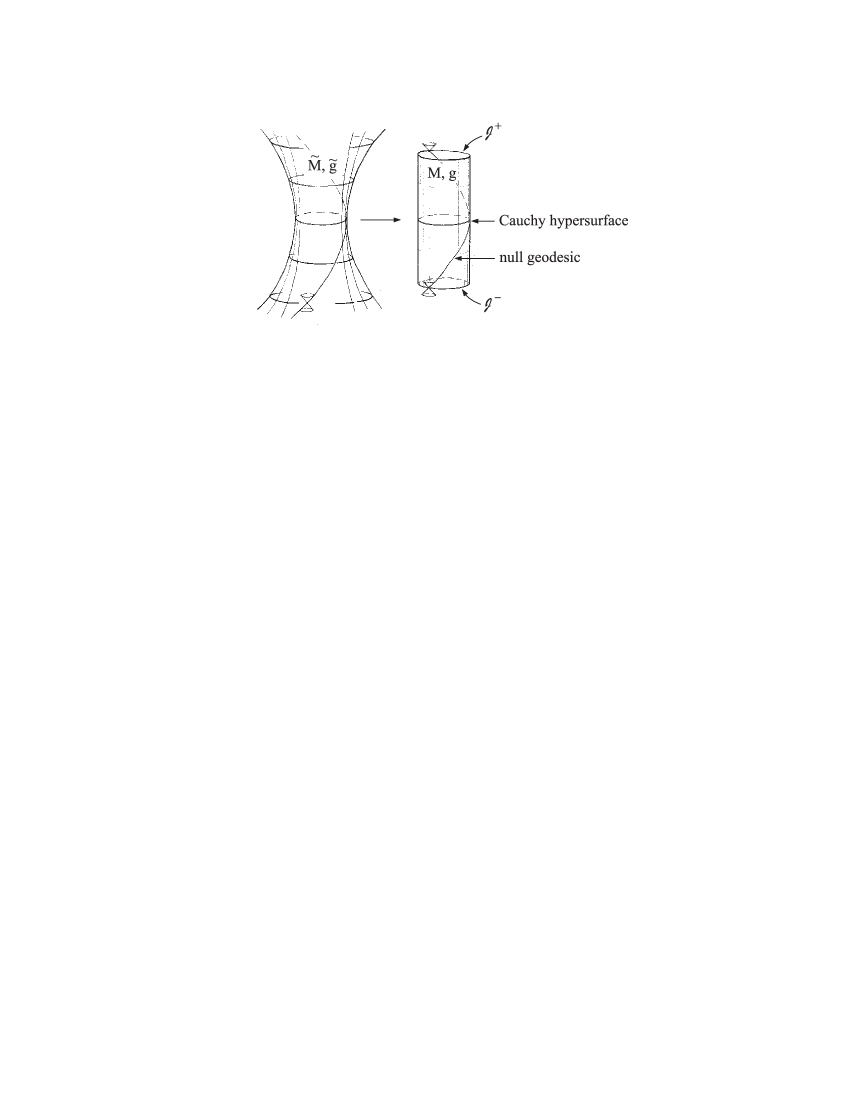
Figure 1: Embedding the physical space-time into its conformal extension.

Pick now any solution of the type considered in the theorem – the standard example is given by De Sitter space – and consider the Cauchy data induced on an arbitrary smooth Cauchy hypersurface of it. If we change these data by a finite but sufficiently small amount, the theorem tells us that these data develop again into a solution satisfying the definition above. Thus the completeness as well as the specific fall-off behaviour of the gravitational field will be preserved. There exist further results which show that this stability property is retained when Einstein’s equations are coupled to conformally well behaved fields like Yang-Mills fields. A reliable estimation of the size of the changes in the data which are admissible here is at present not available. Explicit examples make it clear that we need to impose restrictions.

We emphasize that the asymptotic behaviour of the perturbed solutions asserted in the theorem is implied solely by the choice of data and by the specific properties of Einstein’s equation exhibited below, it is not imposed artificially from outside.

As has been stressed already in [38], [39], the property of asymptotic simplicity is of interest for:

Practical reasons: In many considerations complicated limits in the physical space-time $(\tilde{M},\tilde{g})$ can be replaced by simple differential geometric calculations in the conformal space-time $(M,g)$.

Conceptual reasons: Physical notions based on approximations in the physical space-time can be replaced by notions which are defined in a precise way in terms of fields induced on the conformal boundary ${\cal J}$.

After the idea had been introduced, the further study of asymptotic simplicity concentrated for a long time mainly on these two aspects (cf. the surveys [3], [28]). In view of the theorem above we can now add:

Asymptotic simplicity is a natural concept for solutions to

$$Ric[\tilde{g}]=\lambda\,\tilde{g},\,\,\,\,\,\,\lambda<0,\,\,\,\,\,\,\,\,\,\,\,\,sign(\tilde{g})=(1,-1,-1,-1).$$

We have seen that the asymptotically simple solutions form islands, not singular peaks in the sea of solutions. What is lying in between? Largely uncharted waters. To survey the islands or to explore in any generality what can be found on and beyond their coast lines, we would need to develop new tools. Of course, asymptotically simple space-times have also been studied by the techniques of “exact solutions”. Explicit solutions can locate the islands or allow us to learn about new features of gravitational fields by analysing solutions lying in between. There exist e.g. explicit solutions to (2.1) which develop pieces of a smooth conformal boundary, horizons, and singularities. However, we cannot directly obtain statements about general classes of solutions in this way.

Since “existence” appears to have different meanings for different members of the relativity community, I wish to point out here that in the theorem above I do not simply talk about presumptive solutions of which the first few coefficients in a formal expansion have been determined. Results of the generality considered above are necessarily based on abstract arguments to establish the existence of solutions. Nevertheless, the solutions referred to in this context have the same mathematical “reality” and precision as explicit solutions. I shall have no further reason to consider the field of exact solutions and refer the interested reader to [7] for a survey.

We do not only know by abstract arguments that the space-times considered in the theorem have the very specific asymptotic behaviour asserted there but we can also pinpoint the structural origin of it. Using the fields $g=\Omega^{2}\tilde{g}$ and $\Omega$, and a frame $e_{k}=e^{\mu}\,_{k}\,\partial_{x^{\mu}}$ satisfying $g(e_{i},e_{k})\equiv g_{ik}=diag(1,-1,-1,-1)$, we can derive from Einstein’s equation the “conformal field equations” [14], [15] for the unknowns

$$e^{\mu}\,_{k},\,\,\,\,\,\Gamma_{i}\,^{j}\,{}_{k},\,\,\,\,\,d^{i}\,_{jkl}=\Omega^{-1}\,C^{i}\,_{jkl},\,\,\,\,\,L_{ij}=\frac{1}{2}\,R_{ij}-\frac{1}{12}\,R\,g_{ij},$$

$$\Omega,\,\,\,\,\,\bar{s}=\frac{1}{4}\nabla_{i}\nabla^{i}\Omega+\frac{1}{24}\,R\,\Omega,$$

where $\Gamma_{i}\,^{j}\,{}_{k}$ denotes the connection coefficients in the frame $e_{k}$ and $C^{i}\,_{jkl}$, $R_{ij}$, $R$ the conformal Weyl tensor, the Ricci tensor, and the Ricci scalar of $g$ respectively. The conformal field equations are given by

$$[e_{p},e_{q}]=(\Gamma_{p}\,^{l}\,{}_{q}-\Gamma_{q}\,^{l}\,{}_{p})\,e_{l},$$

$$e_{p}(\Gamma_{q}\,^{i}\,{}_{j})-e_{q}(\Gamma_{p}\,^{i}\,{}_{j})-2\,\Gamma_{k}\,^{i}\,{}_{j}\,\Gamma_{[p}\,^{k}\,{}_{q]}+2\,\Gamma_{[p}\,^{i}\,{}_{|k|}\Gamma_{q]}\,^{k}\,{}_{j}$$

$$=2\,g^{i}\,_{[p}\,L_{q]j}-2\,g^{ik}\,g_{j[p}\,L_{q]k}+\Omega\,d^{i}\,_{jpq},$$

$$\nabla_{i}d^{i}\,_{jkl}=0,$$

$$\nabla_{i}L_{jk}-\nabla_{j}L_{ik}=\nabla_{l}\Omega\,d^{l}\,_{kij},$$

$$\nabla_{i}\,\nabla_{j}\Omega=-\Omega\,L_{ij}+\bar{s}g_{ij},$$

$$\nabla_{i}\bar{s}=-L_{ij}\nabla^{j}\Omega,$$

$$6\Omega\,\bar{s}-3\,\nabla_{j}\Omega\,\nabla^{j}\Omega=\lambda.$$

The derivation of these equations can be found in the literature and I just point out a few of their properties. In regions where $\Omega>0$ the system is equivalent to Einstein’s equation. For the special choice $\Omega\equiv 1$ the last four equations become trivial identities and the first three equations reduce to the system which forms the basis of the Newman-Penrose spin frame formalism [36]. The most important feature of the above system, and in fact the structural background of our results, is the observation that:

The conformal field equations are, in a suitable sense, hyperbolic. This is true irrespective of the sign of $\Omega$.

Two important things are coming together here. The conformal field equations do not contain terms of the form $\Omega^{-1}$, which occur when the Ricci tensor of $g$ is expressed in terms of $\Omega$ and $g$. Secondly, after a suitable choice of gauge conditions the largely overdetermined system above implies symmetric hyperbolic systems of propagation equations which are such that they preserve under their evolution law the constraints which are implied by the system as well. It should be noted that the gauge conditions need to include a condition which determines the conformal factor. A way to impose such a condition is to prescribe the Ricci scalar $R$ of $g$ as a given function on the manifold $M$. The existence results which led to our theorem are based on the hyperbolicity of the conformal field equations.

3 Time-like conformal boundaries

If an asymptotically simple space-time solves Einstein’s equation

$$\tilde{R}_{\mu\nu}=\lambda\,\tilde{g}_{\mu\nu}$$ ((3.1))

near ${\cal J}$, the function $\Omega$ satisfies $g^{\mu\nu}\,\nabla_{\mu}\,\Omega\,\nabla_{\nu}\,\Omega=-\frac{1}{3}\,\lambda$ on ${\cal J}$, i.e. the sign of the cosmological constant determines the causal properties of the conformal boundary [39]. Therefore, if we want to assess the richness of the class of asymptotically simple solutions to Einstein’s equation with $\lambda>0$, for which ${\cal J}$ is time-like, we need to analyse initial boundary value problems where initial data are given on a space-like slice and boundary data are prescribed on the (time-like) conformal boundary ${\cal J}$ at space-like and null infinity (cf. Figure $2$). In terms of the physical space-time this is an unsual initial boundary value problem. The boundary data are to be given on a boundary at space-like and null infinity to be associated with a space-time which is not available yet and which itself is to be determined partly by the boundary data.

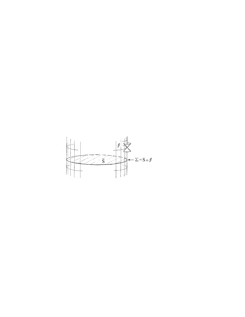
Figure 2: The conformal extension in the case $\lambda>0$.

Nevertheless, this initial boundary value problem can be analysed in detail. Let $\lambda>0$ be given. Data are prescribed on smooth 3-manifolds $\tilde{S}=S\setminus\Sigma$ and ${\cal J}$, where $S$ is an orientable compact manifold with boundary $\Sigma$, ${\cal J}=I\!\!R\times\Sigma$, and we assume $\Sigma$ to be identified with the subset $\{0\}\times\Sigma$ of ${\cal J}$. The data are given as follows:

On $\tilde{S}$ we prescribe smooth, asymptotically simple standard Cauchy data $\tilde{h}_{\mu\nu}$, $\tilde{\chi}_{\mu\nu}$, which satisfy on $\tilde{S}$ the $\lambda$-constraints for space-like hypersurfaces.

Though it should be obvious, we shall explain below the notion of “asymptotic simplicity” for initial data sets more carefully. It restricts the fall-off behaviour of the data near infinity. In the case of the anti-De Sitter covering space, which is the standard example of the situation considered in this chapter, an initial data set of this type is given by $\tilde{S}=I\!\!R^{3}$, $\tilde{\chi}_{\mu\nu}=0$, and a metric $\tilde{h}_{\mu\nu}$ such that $(\tilde{S},-\tilde{h}_{\mu\nu})$ is a simply connected, complete Riemannian space of negative constant curvature.

On ${\cal J}$ we prescribe as boundary data a smooth, 3-dimensional Lorentzian conformal structure for which the slice $\Sigma$ is space-like.

If an initial boundary value problem has a smooth solution, the initial and the boundary data are not quite independent. Thus, without going into details, we require:

The data on $S$ and ${\cal J}$ satisfy the “compatibility conditions” at $\Sigma$ which are implied by the conformal field equations.

Given smooth data on $S$, there is no problem to construct data on ${\cal J}$ such that the compatibility conditions are satisfied.

We set $M=I\!\!R\times S$, perform the obvious identifications ${\cal J}\simeq\partial M$, $\tilde{S}\hookrightarrow S\simeq\{0\}\times S\subset M$, and write $\tilde{M}=M\setminus{\cal J}$. By $t$ we denote the function on $M$, resp. on $\tilde{M}$, which is induced by the projection $M=I\!\!R\times S\rightarrow I\!\!R$. Finally, let $\Omega$ be a smooth function on $M$ with $\Omega>0$ on $\tilde{M}$, $d\,\Omega\neq 0$ on ${\cal J}$. The function it induces on $\tilde{M}$ will also be denoted by $\Omega$. We can state now the following theorem [21].

For given data on $\tilde{S}$ and ${\cal J}$ as described above there is a $T>0$ such that on $\tilde{M}^{\prime}=\{p\in\tilde{M}|\,|t(p)|<T\}$ there exists a unique (up to diffeomorphisms) smooth solution $\tilde{g}$ to $\tilde{R}_{\mu\nu}=\lambda\,\tilde{g}_{\mu\nu}$ which induces the given initial data on $\tilde{S}$ and which is such that $g=\Omega^{2}\,\tilde{g}$ extends to a smooth Lorentz metric on $M^{\prime}=\{p\in M|\,|t(p)|<T\}$ which induces the conformal structure (up to diffeomorphisms) prescribed on $M^{\prime}\cap{\cal J}$.

We have given here a characterization of all smooth asymptotically simple solutions with $\lambda>0$. Our result is global in space in the strong sense that not only the space-like but also the null geodesics which run out to $M^{\prime}\cap{\cal J}$ are complete in that direction. It is only local in time and in fact I did not try to show more; the cases $\lambda>0$ and $\lambda\leq 0$ are distinguished by a fundamental difference in their global causal structures. This statement can be made precise [21] in terms of invariants of the conformal structure.

It is a remarkable feature of the initial boundary value problem above that the data on the boundary can be prescribed in a simple covariant way. This is not the case in the “finite” initial boundary value problem for Einstein’s vacuum field equations where the boundary is thought of as a hypersurface in a smooth vacuum space-time [26]. Nevertheless, apart from the additional freedom which allows us to characterize in the finite problem the location of the boundary, the freedom to prescribe data is the same in both problems. This indicates again the naturalness of the geometric characterization of “infinity” which is inherent in the definition of asymptotic simplicity.

There arise subtleties from the non-compactness of the initial hypersurface $\tilde{S}$. To explain this we need to be more specific about the nature of our data. In the context of initial data “asymptotic simplicity” means the following: (i) The Riemannian space $(\tilde{S},-\tilde{h}_{\mu\nu})$ is conformally compactifiable to a smooth Riemannian space $(S,-h_{\mu\nu})$ for which $\Sigma$ represents the conformal boundary at infinity. (ii) The data $\tilde{h}_{\mu\nu}$, $\tilde{\chi}_{\mu\nu}$ are transformed by the appropriate conformal transformation laws into conformal initial data $h_{\mu\nu}$, $\chi_{\mu\nu}$ which extend smoothly to $\Sigma$. (iii) The conformal initial data set $(S,h_{\mu\nu},\chi_{\mu\nu})$ satisfies those fall-off conditions at $\Sigma$ which are implied by the requirement that it can be embedded smoothly into an asymptotically simple solution to (3.1) as a hypersurface which has intersection $\Sigma=S\cap{\cal J}$ with the conformal boundary and which is space-like everywhere.

The existence of large classes of “free data” which can be used to construct data $h_{\mu\nu}$, $\chi_{\mu\nu}$ satisfying (i) to (iii) follows from [1], [2], [33]. We notice that condition (iii) implies among other things that the conformal Weyl tensor $C^{i}\,_{jkl}$ determined from such data vanishes on $\Sigma$.

There exists a larger class of data which satisfy (i) and (ii) but not (iii). This raises the questions whether the requirement of asymptotic simplicity is inappropriately strong. It turns out, however, that for data violating (iii) the rescaled Weyl tensor $d^{i}\,_{jkl}$ diverges in general strongly at $\Sigma$. Because of the hyperbolicity of the conformal field equations we can expect that this blow up spreads and leads to a space-time with a curvature singularity in which the outgoing null geodesics are not even complete. Questions about their asymptotic behaviour do not arise for such solutions. Moreover, free data yielding data $h_{\mu\nu}$, $\chi_{\mu\nu}$ for which (i) and (ii) hold, need only satisfy a few simple “extra conditions” on $\Sigma$ in order for (iii) to be satisfied. I think it is fair to conclude from what we have seen that:

Asymptotic simplicity is a natural concept for solutions to

$$Ric[\tilde{g}]=\lambda\,\tilde{g},\,\,\,\,\,\,\lambda>0,\,\,\,\,\,\,\,\,\,\,\,\,sign(\tilde{g})=(1,-1,-1,-1).$$

The need for extra conditions on the free data on $\Sigma$ and the fact that data for the conformal field equations explode if these extra conditions are not met, may be forboding complications in the case $\lambda=0$. In that case ${\cal J}$ should be a null hypersurface. It may turn out, however, that the singularity “spreads over the set which we would like to consider as ${\cal J}$” and destroys any hope to find a smooth conformal boundary.

4 Gravitational fields of isolated systems

The idea of the conformal boundary was one of the upshots of a discussion which was initiated by the attempt to arrive at a rigorous concept of gravitational radiation in the context of gravitational fields of isolated systems (cf. [20] for a sketch of this development and a list of relevant references). It is, of course, of utmost interest to control, qualitatively as well as quantitatively, the complete process which starts with the generation of the gravitational radiation by the interactions of some, possibly massive, sources and which ends with the registration of the gravitational radiation at large distances from any sources. At present we are far from a position to do that. However, when I shall concentrate in the following on solutions to the vacuum equations

$$\tilde{R}_{\mu\nu}=0,$$ ((4.1))

it should be kept in mind that the resulting discussion of the asymptotic behaviour of the gravitational field applies also to situations which includes black holes or massive and other sources. These are being ignored here in order not to burden our discussion with a baggage which is irrelevant for the questions we want to analyse.

Our expectation is, of course, that the asymptotic behaviour of the gravtitational field of an isolated system resembles that of Minkowski space. The latter is exhibited most clearly by the well known conformal extension of Minkowski space (cf. Figure $3$).

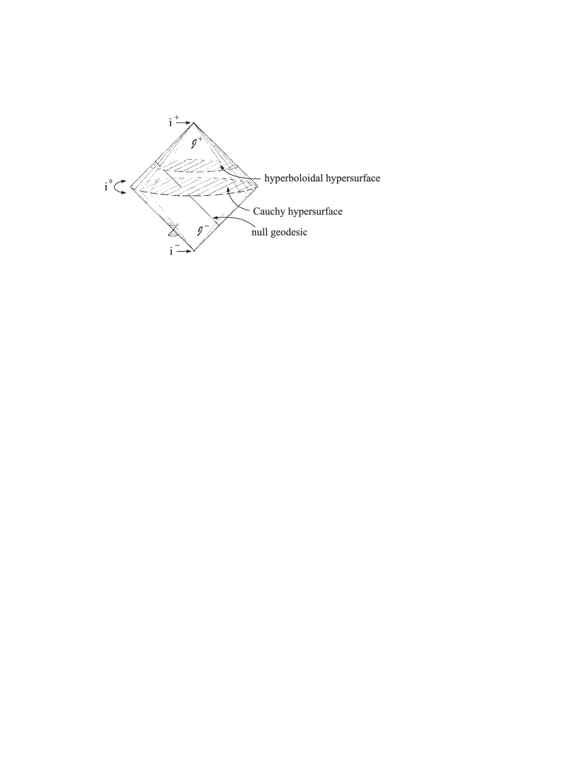
Figure 3: The conformal extension of Minkowski space.

Minkowski space satisfies conditions $1$ to $6$ of our definition of asymptotic simplicity. Moreover, there exist smooth conformal extensions which contain regular points $i^{\pm}$, representing past and future time-like infinity, and a regular point $i^{0}$, which represents space-like infinity. We shall refer to a solution of the Einstein equation (4.1) arising from asymptotically flat initial data on a Cauchy hypersurface diffeomorphic to $I\!\!R^{3}$ and satisfying conditions $1$ to $6$ as to an “Minkowski-type space-time”. The occurence of regular points in the conformal extension corresponding to $i^{\pm}$ will not be required and the occurence of a regular point corresponding to $i^{0}$ cannot be required if we are interested in solutions which are not conformally flat. Nevertheless, we shall follow the custom of thinking of space-like infinity as being represented by an ideal point $i^{0}$. In view of the preceding discussion, one might ask:

Is asymptotic simplicity nonlinearly stable at Minkowski space ?

It turned out to be much more difficult than expected to find an answer to this question. In fact, even the “easier” question whether there exist non-trivial Minkowski-type space-times has not been answered yet.

A first step into that direction was made by the analysis of the hyperboloidal initial value problem. Imagine a smooth hypersurface $S$ in the conformal extension of a Minkowski-type space-time which extends to future null infinity ${\cal J}^{+}$ such that it is space-like even on the boundary $\Sigma=S\cap{\cal J}^{+}$ of $S$. We call such a hypersurface together with the initial data induced on it a “hyperboloidal initial data set” and the initial value problem for Einstein’s equation (4.1) based on these data the “hyperboloidal initial value problem”. The following has been shown [16], [17].

Solutions to the hyperboloidal initial value problem for Einstein’s equation (4.1) are asymptotically simple in the future. Hyperboloidal initial data sufficiently close to Minkowskian hyperboloidal data develop into solutions which admit smooth conformal extensions containing a regular point $i^{+}$ that represents future time-like infinity.

The main point of this result is to reduce the search for Minkowski-type space-times to the investigation of the solutions in a neighbourhood of space-like infinity (thinking in terms of the conformal picture).

An interesting subtlety arises here. It has been shown in [1], [2] how to construct smooth hyperboloidal initial data from suitably given “free data”. Similar to what we have seen in the case $\lambda>0$, there exists also in the present case a class of more general free data which lead to smoothly compactifiable physical initial data. Again, the free data have to satisfy a few extra conditions on the boundary $\Sigma$ of $S$ to yield smooth initial data for the conformal field equations; otherwise the rescaled comformal Weyl tensor determined by them diverges at $\Sigma$. If such divergent data develop at all into solutions which are future null complete, they will certainly not admit a smooth conformal boundary.

Does this indicate the need to impose extra conditions near space-like infinity if we want to construct Minkowski-type space-times from asymptotically flat standard Cauchy data ?

This would be consistent with the results of Christodoulou and Klainerman [8]. In their proof of the nonlinear stability of Minkowski space they could only establish a peeling behaviour of the conformal Weyl tensor near null infinity which is weaker than the peeling behaviour implied by asymptotic simplicity. If their estimates were sharp, this would suggest that asymptotic simplicity can be established only, if at all, for data satisfying stronger conditions then those required in [8].

One may wonder about the possible nature of such conditions. A straightforward strengthening of the usual fall-off conditions of asymptotically flat Cauchy data would eventually lead to data with vanishing mass, i.e. to trivial Cauchy data.

4.1 The basic problem

Our discussion has indicated the importance to understand the behaviour of the field in the region where null infinity touches space-like infinity. To illustrate the situation we take a closer look at space-like infinity in the standard conformal extension of Minkowski space (cf. Figure $4$).

Figure 4: Neighbourhood of $i^{0}$ in Minkowski space.

In this extension the Cauchy hypersurface $\tilde{S}=\{t=0\}$ (say) of Minkowski space is compactified by adding of a point $i$ to obtain a smooth compact hypersurface $S=\tilde{S}\cup\{i\}\simeq S^{3}$. The future (past) null cone at this point coincides with ${\cal J}^{+}$ (${\cal J}^{-}$). It will be convenient conceptually to distinguish the point $i^{0}$, considered as the endpoint of all space-like geodesics in the 4-dimensional space, from the point $i$ representing space-like infinity for the asymptotically flat initial data on $\tilde{S}$. We note that the conformal factor $\Omega$ satisfies $\Omega=0$, $d\,\Omega\neq 0$ on ${\cal J}^{\pm}$ and $\Omega=0$, $d\,\Omega=0$, $Hess\,\Omega\simeq g$ at $i^{0}$.

We could choose now asymptotically flat Cauchy data for Einstein’s equation (4.1) on $\tilde{S}$ which are close to the initial data induced by Minkowski space, transform them appropriately to obtain the corresponding data for the conformal field equations, and try to establish the existence of non-trivial Minkowski-type space-times by using the conformal field equations. Then we encounter the following difficulty, which poses in fact the main problem of the whole field. Let $|x(p)|$ denote the distance of the point $p\in S$ from the point $i$ in terms of the given metric $h_{\mu\nu}$ on $S$. Then one finds that precisely at the point where the mass of the data manifests itself the rescaled conformal Weyl tensor behaves like

$$d^{i}\,_{jkl}=O(\frac{1}{|x|^{3}})\quad\mbox{as}\quad|x|\rightarrow 0\quad\mbox{unless}\quad m_{ADM}=0.$$

This strong divergence at $i$ of some of the initial data for the conformal field equations has the consequence that the existence of Minkowski-type solutions cannot be shown by applying straightforward PDE methods to these equations.

If one tries to analyse the evolution of the field near $i$ one faces a host of complicated subproblems. Already the calculation of a formal expansion of a solution will quickly be swamped by singular terms which get more and more complicated at any order. Moreover, there are various questions which have to be analysed in the context of abstract existence arguments. Just to name a few: (i) How do we choose the gauge ? If the chosen gauge is propagated implicitly by wave equations the singularity at $i$ may lead to singular gauge dependent fields, including $\Omega$, which possibly hide the intrinsic smoothness of the conformal boundary. (ii) How do we control the conformal life time of the solution ? We would need to ensure that the solutions extend smoothly to the set ${\cal J}=\{\Omega=0\}$ but it may already turn out problematic to locate this set if the gauge dependent function $\Omega$ is non-smooth. Finally, how do we decide whether “${\cal J}$ is inherently smooth/non-smooth” ?

Our problem is in fact even more complicated. As mentioned above, it may be necessary to consider a suitably restricted subclass of the Cauchy data considered e.g. in [8] to obtain solutions which admit a smooth structure at null infinity. This poses the difficult question: How do we relate the smoothness of the solution near null infinity to properties of the Cauchy data on $S$ and how do we determine those data which evolve into asymptotically simple space-times ?

In view of these difficulties a different kind of question arises. In zeroth order of the conformal structure, i.e. on the level of the light cone structure or the causal structure, space-like infinity is represented naturally as an ideal point. For higher order structures derived from the conformal structure to be smooth this representation is too narrow. Thus we are led to ask: Does there exist a useful representation of space-like infinity which is “finite but wider than the point $i^{0}$” ?

4.2 The finite representation of space-like infinity

It turns out that the investigation of the questions raised above requires a much deeper analysis of the Cauchy data near space-like infinity as has been available hitherto. What exactly needs to be known can only be decided by a simulteneous study of the evolution problem. In order not to get bogged down by the wealth of details and to be able to concentrate on the evolution problem I worked out the following results for a class of data which is rich enough to exhibit the decisive features of the problem and which, on the other hand, reduces the amount of algebraic calculations considerably. Furthermore, I assume the data to be given on $\tilde{S}=S\setminus\{i\}$ where $S\simeq S^{3}$. It should be emphasized that this condition and the conditions listed below are mainly made for convenience. There is ample space for generalizations and what will be said later on about the evolution equations is independent of requirements on the data. Our assumptions are as follows:

The data are time-symmetric, i.e. $\tilde{\chi}_{\mu\nu}=0$ and the data are specified completely by an asymtotically flat (negative) Riemannian metric $\tilde{h}_{\mu\nu}$ on $\tilde{S}$ with vanishing Ricci scalar. The data are “asymptotically simple”, i.e. there exists a function $\Omega\in C^{\infty}(\tilde{S})\cap C^{2}(S)$ with $\Omega>0$ on $\tilde{S}$, $\Omega=0$, $d\,\Omega=0$, and $Hess\,\Omega$ negative definite at $i$ such that $h_{\mu\nu}=\Omega^{2}\,\tilde{h}_{\mu\nu}$ extends to a smooth Riemannian metric on $S$. In some $h$-normal coordinate system $x^{\alpha}$ centered in $i$ the metric $h_{\mu\nu}$ is real analytic close to $i$.

As a consequence the basic data have the following local expressions near $i$. The conformal factor has the form $\Omega=\frac{|x|^{2}}{(U+|x|\,W)^{2}}$ where $U$, with $U(i)=1$, is an analytic function determined by the local geometry near $i$ and $W$ is an analytic function which encodes global information since $W(i)=\frac{1}{2}\,m_{ADM}$. Writing $\Gamma=|x|^{2}$, the rescaled conformal Weyl tensor takes in space spinor notation the form $\phi_{abcd}=\phi^{\prime}_{abcd}+\phi^{W}_{abcd}$ with a “massles part”

$$\phi^{\prime}_{abcd}=\Gamma^{-2}\,\left\{U^{2}\,D_{(ab}\,D_{cd)}\,\Gamma-4\,U\,D_{(ab}\Gamma\,D_{cd)}U\right.$$

$$\left.-2\,\Gamma\,U\,D_{(ab}\,D_{cd)}\,U+6\,\Gamma\,D_{(ab}U\,D_{cd)}U+\Gamma\,U^{2}\,s_{abcd}\right\},$$

defined in terms of the local geometry near $i$, and a “massive part”

$$\phi^{W}_{abcd}=\Gamma^{-2}\,\left\{-\frac{3}{2}\,\frac{1}{|x|}\,U\,W\,D_{(ab}\,\Gamma\,D_{cd)}\,\Gamma+U\,W\,|x|\,D_{(ab}\,D_{cd)}\,\Gamma\right.$$

$$+2\,|x|\,(W\,D_{(ab}\Gamma\,D_{cd)}U-3\,U\,D_{(ab}\Gamma\,D_{cd)}W)$$

$$+2\,|x|\,\Gamma\,(-U\,D_{(ab}\,D_{cd)}\,W-W\,D_{(ab}\,D_{cd)}\,U+6\,D_{(ab}U\,D_{cd)}\,W+U\,W\,s_{abcd})$$

$$\left.+\Gamma^{2}\,(-2\,W\,D_{(ab}\,D_{cd)}\,W+6\,D_{(ab}W\,D_{cd)}\,W+W^{2}\,s_{abcd})\right\},$$

where $s_{abcd}$ denotes the trace free part of the Ricci tensor of $h$. Unless the ADM mass vanishes we still have $\phi^{W}_{abcd}=O(\frac{1}{|x|^{3}})$ as $|x|\rightarrow 0$.

Analysing under these assumptions the situation near space-like infinity and letting oneself be guided by the field equations and conformal geometry, one is led to a representation of space-like infinity which differs from anything suggested before. The new picture is indicated in Figure $5$.

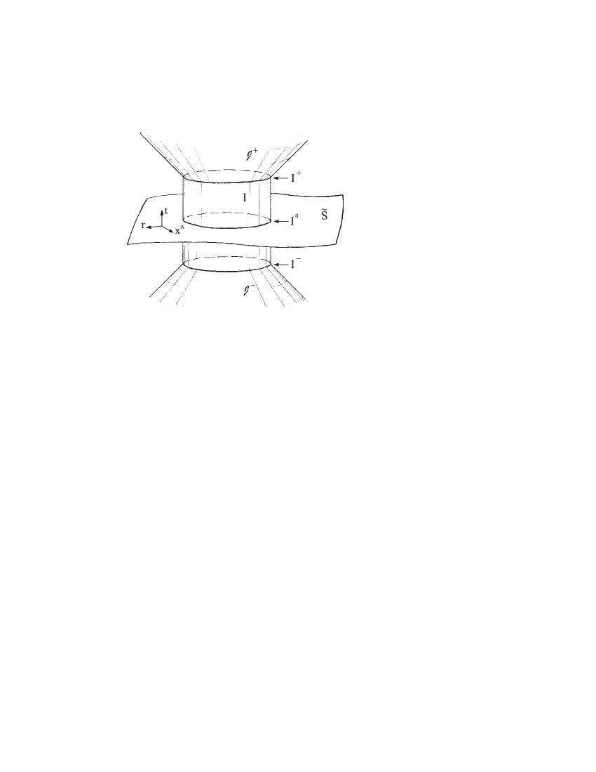
Figure 5: The cylinder $I$ representing space-like infinity.

It is an important element of this setting that the conformal factor, denoted by $\Theta$ to distiguish it from the function $\Omega$ given on the initial hypersurface $S$, is known explicitly as a function of the coordinates and the initial data on $\tilde{S}$. As we shall see, it is determined completely by the conformal geometry, Einstein’s equation, and certain initial conditions on $\tilde{S}$ which are chosen here such as to obtain a simple picture.

The point $i\in S$ is blown up to a spherical set $I^{0}\simeq S^{2}$ which forms the new boundary of $\tilde{S}$ at space-like infinity. We write now $S=\tilde{S}\cup I^{0}$ for the smooth manifold with boundary $I^{0}$ so obtained and introduce a coordinate $r$ on $S$ which vanishes on $I^{0}$ and is positive elsewhere.

The coordinate $t$ is chosen such that it vanishes on $S$ and induces an intrinsic parameter on a congruence of “conformal geodesics” orthogonal to $S$. Then the 4-dimensional space-time $\tilde{M}$ is given near space-like infinity in the form $\tilde{M}=\{(t,p)\in I\!\!R\times S|r(p)>0,\,\,\,|t|<1+r(p)\}$. We have $\Theta>0$ on $\tilde{M}$.

By a natural extension process we obtain the set $I=\{(t,p)\in I\!\!R\times S|r(p)=0,\,\,\,|t|<1\}$ which represents space-like infinity. In terms of the earlier picture a point of $I$ can be interpreted as a space-like direction at $i^{0}$, but $I$ is not defined this way. Furthermore, future and past null infinity are given near space-like infinity by the sets ${\cal J}^{\pm}=\{(t,p)\in I\!\!R\times S|r(p)>0,\,\,\,t=\pm(1+r(p))\}$. The function $\Theta$ vanishes on $I\cup{\cal J}^{-}\cup{\cal J}^{+}$. The set $I^{\pm}=\{(t,p)\in I\!\!R\times S|r(p)=0,\,\,\,t=\pm 1\}$, where “null infinity touches space-like infinity”, will be of special interest. In the following I shall indicate the structural background of the new picture.

4.3 Conformal geometry and Einstein’s equation

One of the most important features of the new representation is that it is defined exclusively in terms of the field equations and the conformal geometry or, equivalently, the light cone structure which in turn determines the physical characteristics of the field equations. To make full use of the conformal geometry we need to consider conformal rescalings $\tilde{g}\rightarrow g=\Theta\,\tilde{g}$ of the metric as well as transitions from the $\tilde{g}$-Levi-Civita connection to “Weyl connections” $\tilde{\nabla}\rightarrow\hat{\nabla}=\tilde{\nabla}+S(b)$, where the difference tensor, determined by a 1-form $b$, is defined by $S(b)_{\mu}\,^{\nu}\,{}_{\rho}=\delta^{\nu}\,_{\mu}\,b_{\rho}+\delta^{\nu}\,_{\rho}\,b_{\mu}-\tilde{g}_{\mu\rho}\,\tilde{g}^{\nu\lambda}\,b_{\lambda}$. Parallel transport by such connections maps $\tilde{g}$-conformal frames again into such frames.

A “conformal geodesic” [43] is a space-time curve $x(t)$, together with a 1-form $b(t)$ along it, which satisfy the system of ODE’s

$$(\tilde{\nabla}_{\dot{x}}\dot{x})^{\mu}+S(b)_{\nu}\,^{\mu}\,{}_{\rho}\,\dot{x}^{\nu}\,\dot{x}^{\rho}=0,\,\,\,\,\,(\tilde{\nabla}_{\dot{x}}b)_{\nu}-\frac{1}{2}b_{\mu}\,S(b)_{\nu}\,^{\mu}\,{}_{\rho}\,\dot{x}^{\rho}-\tilde{L}_{\nu\mu}\,\dot{x}^{\mu}=0,$$

where $\tilde{L}_{\nu\mu}=\frac{1}{2}\,(\tilde{R}_{\nu\mu}-\frac{1}{6}\,\tilde{g}_{\nu\mu}\,\tilde{R})$ is given in terms of the Ricci tensor and the Ricci scalar of $\tilde{g}$.

The 1-form $b(t)$ defines by the formula above a Weyl connection $\hat{\nabla}$ along the curve $x(t)$ such that the curve is an autoparallel for this connection. It is important to note that the curve $x(t)$ and the connection $\hat{\nabla}$ are invariants of the conformal structure of $\tilde{g}$.

We construct in an obvious way “conformal Gauss coordinates based on $S$” [27] which are generated by a congruence of conformal geodesics threading orthogonally through $S$. The natural parameter $t$ on these curves which vanishes on $S$ is used as a time coordinate. Beside the connection $\hat{\nabla}$ we introduce also a smooth conformal frame field $e_{k}$ which satisfies $\hat{\nabla}_{\dot{x}}\,e_{k}=0$. This defines in turn a metric $g$ in the conformal class of $\tilde{g}$ by the requirement $g_{ik}\equiv g(e_{i},e_{k})=diag\,(1,-1,-1,-1)$ and consequently a conformal factor $\Theta$ satisfying $g=\Theta^{2}\,\tilde{g}$.

By this procedure we obtain a “conformal Gauss gauge” which is defined solely in terms of conformal geometry. We study this gauge because we expect that suitably chosen conformal geodesics starting in the physical space-time will pass through null infinity into the (prospective smooth) conformal extension without being affected by the singularity at the point $i$. The freedom to prescribe on $S$ initial data for $\dot{x}$, $b$, $e_{k}$, whence for $\Theta$, can be used to adapt the gauge to the situation we want to study.

The attempt to combine this gauge with the conformal field equations led to the following unexpected observation [21].

Suppose $x(t)$, $b(t)$, $e_{k}(t)$, $\Theta(t)$ are as above with $t$ taking values in an interval $J$, $x(t)$ being time-like, and $\dot{x}(t_{*})=e_{0}$, $\Theta(t_{*})>0$ for some $t_{*}\in J$. Then, if Einstein’s equation $\tilde{R}_{\mu\nu}=0$ holds on $\tilde{M}$, one has

$$\Theta(t)=\Theta_{*}+(t-t_{*})\,\dot{\Theta}_{*}+\frac{1}{2}\,(t-t_{*})^{2}\,\ddot{\Theta}_{*},\,\,\,\,\,\,\,d_{k}(t)\equiv\Theta\,b_{\mu}\,e^{\mu}\,_{k}=(\dot{\Theta},d_{a*})$$

with constants $\Theta_{*}$, $\dot{\Theta}_{*}$, $\ddot{\Theta}_{*}$, $d_{a*}$, $a=1,2,3$.

Thus the conformal factor $\Theta$ is known explicitly as a function of the parameter $t$ and certain data at $t_{*}$. Moreover, it is quadratic in $t$ and, provided the underlying conformal geodesic has a sufficiently long life-time, we can expect that there are numbers $t_{\pm}\in J$, $t_{-}<t_{*}<t_{+}$ with $\Theta(t_{\pm})=0$. This is precisely what would happen if $x(t)$ would pass the conformal boundary at $t_{\pm}$, i.e. if we had $x(t_{\pm})\in{\cal J}^{\pm}$.

There is some information about Einstein’s equation (4.1) encoded in the expressions for $\Theta(t)$, $d_{k}(t)$. Under the assumption that the congruence of conformal geodesics passes smoothly through ${\cal J}$, the expressions imply $g^{ij}\,\nabla_{i}(\Theta)\,\nabla_{j}(\Theta)=0$ on ${\cal J}$, a relation which was deduced before from the field equations.

To incorporate the conformal Gauss gauge into the field equations we need to extend the conformal field equations to admit Weyl connections. The “generalized conformal Einstein equations” so obtained form a system of equations for the unknown

$$u=\left(e^{\mu}\,_{k},\,\hat{\Gamma}_{i}\,^{j}\,{}_{k},\,\hat{L}_{jk}=\frac{1}{2}\,\hat{R}_{(jk)}-\frac{1}{12}\,\hat{R}\,g_{jk}-\frac{1}{4}\,\hat{R}_{[jk]},\,d^{i}\,_{jkl}=\Theta^{-1}\,C^{i}_{jkl}\right),$$

where $\hat{\Gamma}_{i}\,^{j}\,{}_{k}$ are the connections coefficients of the Weyl connection $\hat{\nabla}$ in the frame $e_{k}$, $\hat{R}_{jk}$ is the Ricci tensor of $\hat{\nabla}$, and $\hat{R}$ = $g^{jk}\,\hat{R}_{jk}$. The system is given by

$$[e_{p},e_{q}]=(\hat{\Gamma}_{p}\,^{l}\,{}_{q}-\hat{\Gamma}_{q}\,^{l}\,{}_{p})\,e_{l},$$

$$e_{p}(\hat{\Gamma}_{q}\,^{i}\,{}_{j})-e_{q}(\hat{\Gamma}_{p}\,^{i}\,{}_{j})-2\,\hat{\Gamma}_{k}\,^{i}\,{}_{j}\,\hat{\Gamma}_{[p}\,^{k}\,{}_{q]}+2\,\hat{\Gamma}_{[p}\,^{i}\,{}_{|k|}\,\hat{\Gamma}_{q]}\,^{k}\,{}_{j}$$

$$=2\,g^{i}\,_{[p}\,\hat{L}_{q]j}-2\,g^{ik}\,g_{j[p}\,\hat{L}_{q]k}-2\,g^{i}\,_{j}\,\hat{L}_{[pq]}+\Theta\,d^{i}\,_{jpq},$$

$$\nabla_{i}\,d^{i}\,_{jkl}=0,$$

$$\hat{\nabla}_{p}\,\hat{L}_{qj}-\hat{\nabla}_{q}\,\hat{L}_{pj}=d_{i}\,d^{i}\,_{jpq}.$$

We note that no differential equations for the fields $\Theta$, $d_{k}$ are included. For our purpose the most important property of this system is stated in the following result [21].

In the conformal Gauss gauge, with $\Theta(t)$, $d_{k}(t)$ being the explicit expressions above, the generalized conformal Einstein equations imply a “reduced system” of evolution equations which (i) is symmetric hyperbolic irrespective of the values taken by $\Theta$, (ii) preserves the constraints under its evolution, (iii) gives for initial data satisfying the constraints solutions $\tilde{g}_{\mu\nu}=\Theta^{-2}\,g_{\mu\nu}$ to Einstein’s equation (4.1) in the region where $\Theta>0$.

The conformal factor $\Theta$ and the 1-form $d_{k}$ play the role of gauge source functions in the equations (cf. [22]). The propagation equations for the fields $e^{\mu}\,_{k}$, $\hat{\Gamma}_{i}\,^{j}\,{}_{k}$, $\hat{L}_{jk}$ contain only the derivative operator $\partial_{t}$. This simplifies the analysis near $i$ considerably and clearly exhibits the special status of the Bianchi equation.

Given the equations above, it turns out that one can adapt the conformal Gauss gauge in a particularly convenient way to the situation near space-like infinity. All the details which are to be observed here and also the following results can be found in [23]. I mention just one basic choice. We set $\Theta=\Theta_{*}\equiv\kappa^{-1}\,\Omega$, $b=\Omega^{-1}\,d\,\Omega$ on $\tilde{S}$ with $\kappa=r\,\kappa^{\prime}$ where $\kappa^{\prime}$ is smooth and satisfies $\kappa^{\prime}(i)=1$. Here $r(p)$ denotes the $h$-distance of a point $p\in S$ from $i$. Assuming in addition $d_{\mu}\,e^{\mu}\,_{0}=0$ on $\tilde{S}$, the fields $\Theta$, $b$ are determined on $\tilde{M}$ and its possibly smooth conformal extensions. We note that the conformal gauge on $\tilde{M}$ given by $\Theta$ is related in a particular way to the conformal gauge of the initial data specified by $\Omega$.

We perform now the blow up by which the point $i$ is replaced by the sphere $I^{0}$ and use $r$ to define a coordinate, again denoted by $r$, which vanishes on $I^{0}$ and is positive on $S\setminus I^{0}$. We shall consider below an extension of $S$ beyond $I^{0}$ which is defined by allowing $r$ to take negative values. When the complete set of initial data for the generalized conformal Einstein equations is transferred appropriately to the new setting we find the following surprising result.

The function $\kappa^{\prime}$ can be chosen such that $\Theta=\Theta_{*}\,\left(1-\frac{t^{2}}{(1+r)^{2}}\right)$, with $\Theta_{*}$ constant along the conformal geodesics, and such that $\Theta$, $d_{k}$ can be extended smoothly into a region where $r\leq 0$. Moreover, the initial data for the generalized conformal Einstein equations can be extended smoothly into a domain where $r\leq 0$.

This observation allows us to set up a regular, finite initial value problem near space-like infinity which gives the new picture of space-like infinity outlined above. The set $I$ representing space-like infinity is obtained in our gauge by a simple smooth extension and, if the solution extends smoothly to the set $\{t=\pm(1+r)\}$, a conformal boundary ${\cal J}$ is obtained by a smooth extension as well.

4.4 The cylinder $I$ at space-like infinity

In the following I want to discuss the nature of the finite, regular initial value problem at space-like infinity and some of the consequences which have been worked out so far [23]. Since it is defined exclusively in terms of the conformal geometry, this initial value problem “is always there”. We can ignore it but we cannot avoid its consequences. Any results derived from it gives direct information on the conformal geometry.

Since the data and the equations extend smoothly into the set $\{r\leq 0\}$, we get on the closure of $\tilde{M}$ a problem for symmetric hyperbolic equations of the form

$$(A^{t}\,\partial_{t}+A^{r}\,\partial_{r}+A^{B}\,\partial_{B})\,u=F(t,r,x^{A};u),$$

with matrix valued functions $A^{\mu}$ of the unknown “vector”$u$ and the coordinates $x^{0}=t$, $x^{1}=r$, $x^{A}$, $A=1,2$, where the latter imply in particular local coordinates on the sphere $I^{0}$.

A curious property of the new problem is the occurrence of the “boundary” $I$. To understand its nature we extend the initial data and the equations smoothly into the region $\{r\leq 0\}$ and use the well known results on symmetric hyperbolic equations (cf. [35], [41]) to establish the existence of a smooth solution in some neighbourhood $U$ of the extended initial hypersurface $S$. Obviously $U$ includes a part of $I$. Given this solution, we can conclude from the form of the equations and the data that

The cylinder $I$ at space-like infinity is “totally characteristic” in the sense that $A^{r}=0$ on $I$.

Restricting our propagation equations to $I$ we thus get interior symmetric hyperbolic equations $(A^{t}\,\partial_{t}+A^{B}\,\partial_{B})\,u=F(t,0,x^{A};u)$ on $I$ which allow us to determine $u$ on $I$ uniquely in terms of the values of $u$ on $I^{0}$. It follows, as expected, that the solution is determined on $\tilde{M}\cap U$ uniquely by the data on $\tilde{S}$. The extension of our original problem into the range where $r<0$ is just a convenient trick to establish the existence of a solution which extends smoothly to $I\cap U$.

For $p=0,1,2,\ldots$ we denote by $u_{p}=\partial^{p}_{r}\,u|_{I}$ the restriction of the $p$-th $r$-derivative of $u$ to $I$. Taking formal $r$-derivatives of our original propagation equations and restricting to $I$, we find

The quantities $u_{p}$, $p=1,2,\ldots$, can be determined on $I$ recursively as solutions to linear symmetric hyperbolic equations on $I$. The formal expansion $u=\sum_{p\geq 0}\frac{1}{p!}\,u_{p}(t,x^{A})\,r^{p}$ of $u$ defined by these coefficients on $I$ is convergent in a neighbourhood of $I^{0}$.

We can calculate recursively explicit formulae for the quantities $u_{p}$. Though the expressions become more and more complicated for increasing $p$ and we are still far from having worked out all the details we can state the most important consequence of the observation above.

The interior equations on $I$ allow us to relate properties of the solution on ${\cal J}^{\pm}$ near $I^{\pm}$ to the structure of the data on $S$ near $I^{0}$ if the solution extends smoothly to ${\cal J}^{\pm}$.

As an example, J. Kánnár [34] has derived (observing the regularity condition given below) formulae for the conserved quantities of Newman and Penrose [37] in terms of the functions $u_{p}$, $p=0,\ldots,3$. Another example is given by the following result. Since the total characteristic $I$ approaches the characteristic ${\cal J}^{\pm}$ transversely in $I^{\pm}$ we can expect a degeneracy of the equations on this set. The calculation of $u$ on $I$ shows in fact that the matrix $A^{t}$, which is positive definite on $I$, degenerates on $I^{\pm}$. As a consequence the functions $u_{p}$ develop a certain type of logarithmic singularity on $I^{\pm}$. For a correct assessment of this observation it is important that our setting is defined completely in terms of the conformal geometry and not based on some obscure gauge condition. The observed singularities indicate an intrinsic property of the conformal structure. It turns out that we can isolate those parts of the initial data which give rise to the singular terms.

The logarithmic singularities alluded to above do not occur if $h$ satisfies at the point $i$ the regularity condition

$${\cal C}(D_{i_{1}},\dots,D_{i_{p}}\,B_{jk})(i)=0,\,\,\,\,\,p=0,1,2,\ldots,$$

where $B_{jk}$ denotes the Cotton tensor of $h$ and ${\cal C}$ means “symmetrize and take the trace free part”. This regularity condition is equivalent to the requirement that the massless part $\phi^{\prime}_{abcd}$ of the rescaled conformal Weyl tensor extend smoothly to the point $i$ of the initial hypersurface.

The regularity condition is conformally invariant and thus in fact a condition on the free initial data. Complicated as it looks, the condition is in fact quite weak and appears to impose hardly any restriction on the modeling of physically interesting systems. It allows us to choose the free data arbitrarily on any given compact subset of $\tilde{S}$, provided we observe, as usual, the solvability of the Lichnerowicz equation. Furthermore, the condition is satisfied by all static solutions which are analytic at space-like infinity [5], [18]. Thus it implies no restriction on the admissible multipoles.

We note, that the set $I$ is obtained as a limit of conformal geodesics and that its points can be interpreted as the “space-like directions at $i^{0}$”. Apart from that it does not have any geometric meaning. The light cone structure degenerates on $I$ but the vector fields used to express the equations extend smoothly to $I$. We find that $g(\partial_{r},\partial_{r})(p)\rightarrow\infty$ as $p\rightarrow I$, $|t(p)|<1-\epsilon$, $0<\epsilon<1$. If we replace $r$ by a radial coordinate $\rho$ which is better adapted to the conformal gauge defined by $\Theta$ in the sense that $0<c<g(\partial_{\rho},\partial_{\rho})<c^{\prime}<\infty$ we find that $\rho\rightarrow\infty$ as $r\rightarrow 0$. Thus

In terms of coordinates $\rho$, $t$ adapted to the conformal gauge defined by $\Theta$, the set $I$ is at $\rho=\infty$ but “has finite circumference”. The set ${\cal J}^{\pm}$ is finite in time $t$.

It is a remarkable fact that the field $d_{k}$ and the coordinate $r$, which are adapted to the conformal factor $\Omega$, conspire with the conformal gauge defined by $\Theta$ to provide a smooth finite representation of space-like infinity. We thus arrived at the picture of an isolated system indicated in Figure $6$.

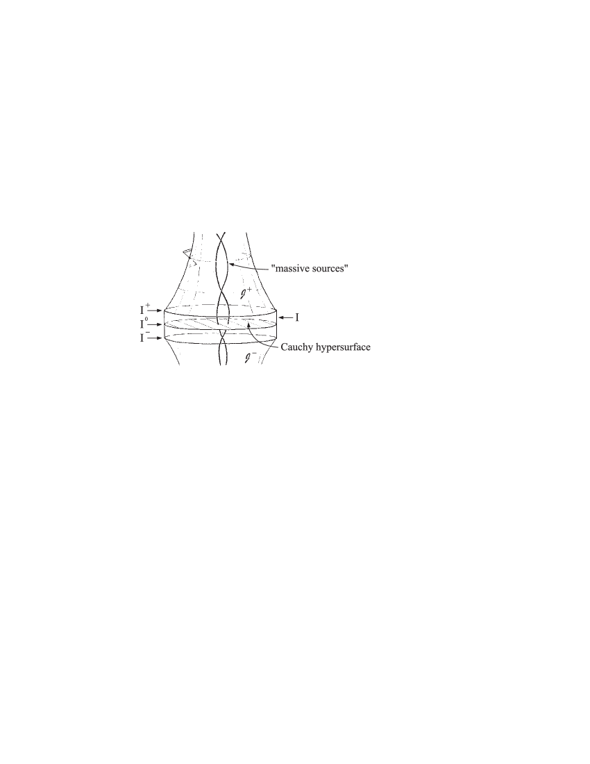
Figure 6: An isolated gravitating system in the new representation.

A detailed comparison of the analysis of space-like infinity outlined in this lecture with other investigations of space-like infinity (cf. [3], [4], [6], [8], [9], [40]) is impossible here. Naturally, all these studies have various aspects in common. The present work differs from the work quoted above in that it combines the following features in one approach. The picture of space-like infinity which is proposed here is based on assumptions on the initial data, the structure of the field equations, and properties of conformal geometry. No a priori assumptions on the time evolution are being made. It is designed as a basis for an existence theorem which should enable us to derive statements about the smoothness of the structure at null infinity. This theorem has still to be worked out. If it will be done, the setting will allow us to analyse the consequences of the field equations near space-like infinity to an arbitrary precision and we shall be able to relate qualitative and quantitative properties of the fields on ${\cal J}$ near space-like infinity to the structure of the initial data. Moreover, the setting has the important practical feature that the evolution of the fields can be studied in a finite picture near space-like and null infinity with the usual concepts of smoothness.

5 Concluding Remarks

The conformal structure proved to be most important in deriving – on the level of differential topology and geometry – statements on the behaviour of space-times in the large. The discussion above shows clearly that it is of structural interest to understand the interaction between conformal geometry and Einstein propagation in depth. Our statements above about the existence and the behaviour of solutions in the large were obtained by results concerning this relation. There is still much more to be learned about it.

Though it has not been emphasized above, certain results about the hyperbolicity of the Einstein equations form an important technical ingredient in our analysis. Since the conformal field equations contain the Bianchi identity as a central part, hyperbolic reductions of the Einstein equations based on equations for the curvature tensor play a vital role in our discussions. Since the Bianchi identity is a tensor equation, the hyperbolicity of the propagation equations derived from it is independent of the gauge conditions imposed on the lower order fields and the formalism used (frame formalism, spin frame formalism, ADM representation of the metric etc.). There is a considerable variety of possibilities to impose gauge conditions such that the coupled system governing the curvature and the lower oder fields is symmetric hyperbolic. These reductions can conveniently be adapted to characteristic initial value problems, Cauchy problems, and initial boundary value problems (cf. [22] and the references given there). Their applicability is not restricted to the vacuum or the conformal vacuum equations, they can be extended to include matter fields. Recently they have been used for the coupled Einstein-Euler equations to combine symmetric hyperbolicity with a Lagrangian representation of the flow field [25].

We have seen how to derive by straightforward calculations on the cylinder at space-like infinity information about the asymptotic behaviour of solutions in the region where null infinity touches space-like infinity. However, the fact that infinite problems for Einstein’s equations can be converted into regular finite problems for the conformal field equations is of even more practical interest. It offers the possibility to calculate numerically entire asymptotically flat space-times together with their conformal boundary on finite grids. The introduction of cut-offs of the field at artificial time-like boundaries is not necessary. By a judicious choice of the space-like slicing in the neighbourhood of the cylinder $I$ it should be possible to perform a smooth transition from the standard Cauchy problem for the conformal field equations to the hyperboloidal Cauchy problem.

Numerical calculations based on the hyperboloidal Cauchy problem have been performed successfully by Hübner [29], [30], [31], [32] and Frauendiener [12], [13]. The full potential of hyperboloidal hypersurfaces, which offer a convenient way to trace radiation in the context of Cauchy problems, can only completely be exhausted in conjuction with the conformal field equations. The radiation extraction is performed directly at null infinity where a well defined concept of a “radiation field” is available [38], [39].

The fact that the requirement of smoothness of the fields near $I^{\pm}$ implies regularity conditions on the data raises new questions about the concept of an “isolated system” in general relativity (cf. also [24] for a discussion of this point). Several authors (cf. [10], [42]) considered asymptotic expansions of the gravitational field near null infinity which admit logarithmic terms. I think that one should not give in so easily. We have seen that the somewhat esoteric desire to get control on the asymptotic smoothness of solutions yields results of immediate practical consequences. Moreover, the idea of an “isolated system” is an idealization which introduces “space-like infinity” as a convenient construct. These notions leave a certain freedom which should be exploited as far as necessary but without introducing irrelevant information. If in the end it should turn out that the requirement of asymptotic simplicity restricts the class of admissible solutions too strongly to model certain situations of physical interest, we will have understood why there is a need to generalize and can start to do so.

Perhaps also Ellis’s critique [11] of the notion of an isolated system considered in this lecture should be mentioned here. It was argued in [11] that one should avoid this idealization, seperate instead the system of interest (star, system of stars etc.) from the rest of the universe by a cut along a time-like hypersurface and study the system so obtained. This introduces an initial boundary value problem into the discussion of the system. Apart from the fact that it is hard to see how we could get useful information on the required boundary data, this problem introduces difficulties of its own [26]. In view of this and the results discussed above it appears to me that at least the technical aspects of the critique in [11] need to be reconsidered in the light of the recent developments.

References

- [1] L. Andersson, P.T. Chruściel, H. Friedrich. On the regularity of solutions to the Yamabe equation and the existence of smooth hyperboloidal initial data for Einstein’s field equations. Commun. Math. Phys., 149 (1992) 587 - 612.
- [2] L. Andersson, P.T. Chruściel. On “Hyperboloidal” Cauchy Data for Vacuum Einstein Equations and Obstruction to the Smoothness of Scri. Commun. Math. Phys., 161 (1994) 533 - 568.
- [3] A. Ashtekar. Asymptotic properties of isolated systems: Recent developments. In: General Relativity and Gravitation B. Bertotti et. al (eds.), Reidel, Dordrecht, 1984.
- [4] A. Ashtekar, J.D. Romano. Spatial infinity as a boundary of space-time. Class. Quantum Grav., 9 (1992) 1069 - 1100.
- [5] R. Beig. Conformal properties of static space-times. Class. Quantum Grav. 8 (1991) 263 - 271.
- [6] R. Beig, B.G. Schmidt. Einstein’s Equations near Spatial Infinity. Commun. Math. Phys., 87 (1982) 65 - 80.
- [7] J. Bičák. Radiative spacetimes: Exact approaches. In: Relativistic Gravitation and Gravitational Radiation J.-A. Marck, J.-P. Lasota (eds.), Cambridge University Press 1997.
- [8] D. Christodoulou, S. Klainerman. The Global Nonlinear Stability of the Minkowski Space. Princeton University Press, Princeton 1993.
- [9] P.T. Chruściel. On the Structure of Spatial Infinity: II. Geodesically Regular Ashtekar-Hansen Structures. J. Math. Phys. 30 (1989) 2094 - 2100.
- [10] P.T. Chruściel, M. A. H. MacCallum, D. B. Singleton. Gravitational Waves in General Relativity. XIV: Bondi Expansions and the “Polyhomogeneity” of . Phil. Trans. Royal Soc, London, A 350 (1995) 113 - 141.
- [11] G. F. R. Ellis. Relativistic Cosmology: Its Nature, Aims, and Problems. In: General Relativity and Gravitation B. Bertotti et. al (eds.), Reidel, Dordrecht, 1984.
- [12] J. Frauendiener. Numerical treatment of the hyperboloidal initial value problem for the vacuum Einstein equations I. The conformal field equations. gr-qc/9712050
- [13] J. Frauendiener. Numerical treatment of the hyperboloidal initial value problem for the vacuum Einstein equations II. The evolution equations. gr-qc/9712052
- [14] H. Friedrich. On the regular and the asymptotic characteristic initial value problem for Einstein’s vacuum field equations. In: Proceedings of the Third Gregynoc Relativity Workshop M. Walker (ed.), Max-Planck Green Report MPI-PAE/Astro 204, (1979), Proc. Roy. Soc., A 375 (1981) 169 - 184.
- [15] H. Friedrich. The asymptotic characteristic initial value problem for Einstein’s vacuum field equations as an initial value problem for a first-order quasilinear symmetric hyperbolic system. Proc. Roy. Soc., A 378 (1981) 401 - 421.
- [16] H. Friedrich. Cauchy Problems for the Conformal Vacuum Field Einstein in General Relativity. Commun. Math. Phys., 91 (1983) 445 - 472.
- [17] H. Friedrich. On the existence of n-geodesically complete or future complete solutions of Einstein’s field equations with smooth asymptotic structure. Commun. Math. Phys., 107 (1986) 587 - 609.
- [18] H. Friedrich. On static and radiative space-times. Commun. Math. Phys., 119 (1988) 51 - 73.
- [19] H. Friedrich. On the global existence and the asymptotic behaviour of solutions to the Einstein-Maxwell-Yang-Mills equations. J. Diff. Geom., 34 (1991) 275 - 345.
- [20] H. Friedrich. Asymptotic Structure of Space-Time. In: Recent Advances in General Relativity A. I. Janis, J. R. Porter (eds.), Birkhäuser, Basel, 1992.
- [21] H. Friedrich. Einstein Equations and Conformal Structure: Existence of Anti-de Sitter-Type Space-Times. J. Geom. Phys., 17 (1995) 125 - 184.
- [22] H. Friedrich. Hyperbolic reductions for Einstein’s equations. Class. Quantum Gravity, 13 (1996) 1451 - 1469.
- [23] H. Friedrich. Gravitational fields near space-like and null infinity. J. Geom. Phys., 24 (1998) 83 - 163.
- [24] H. Friedrich. Einstein Equations and Conformal Structure. In: The Geometric Universe: Science, Geometry and the Work of Roger Penrose S. A. Hugget et al. (eds.), Oxford University Press, Oxford, 1998.
- [25] H. Friedrich. Evolution equations for gravitating ideal fluid bodies in general relativity. Phys. Rev. D, 57 (1998) 2317 - 2322.
- [26] H. Friedrich, G. Nagy. The initial boundary value problem for Einstein’s vacuum field equation. Preprint (1998).
- [27] H. Friedrich, B.G. Schmidt. Conformal geodesics in general relativity. Proc. R. Soc. Lond., A 414 (1987) 171 - 195.
- [28] R. Geroch. Asymptotic Structure of Space-Time. In: Asymptotic Structure of Space-Time B. F. P. Esposito, L. Witten (eds.), Plenum Press, New York, 1977.
- [29] P. Hübner. Numerische und analytische Untersuchungen von (singulären) asymptotisch flachen Raumzeiten mit konformen Techniken. Thesis, Universität München 1993.
- [30] P. Hübner. General relativistic scalar-field models and asymptotic flatness. Class. Quantum Grav. 12 (1995) 791 - 808.
- [31] P. Hübner. Method for calculating the global structure of (singular) spacetimes. Phys. Rev. D 53 (1996) 701.
- [32] P. Hübner. Black hole space-times on grids with trivial boundaries. Preprint
- [33] J. Kánnár. Hyperboloidal initial data for the vacuum Einstein equations with cosmological constant. Class. Quantum Grav. 13 (1996) 3075 - 3084.
- [34] J. Kánnár. Private communication (1997).
- [35] T. Kato. The Cauchy problem for quasi-linear symmetric hyperbolic systems. Arch. Ration. Mech. Anal., 58 (1975) 181 - 205.
- [36] E. T. Newman, R. Penrose. An Approach to Gravitational Radiation by a Method of Spin Coefficients. J. Math. Phys. 3 (1992) 566 - 578.
- [37] E. T. Newman, R. Penrose. New Conservation Laws for Zero-Rest-Mass Fields in Asymptotically Flat Space-Time. Proc. Roy. Soc. A 305 (1968) 175 - 204.
- [38] R. Penrose. Asymptotic properties of fields and space-time. Phys. Rev. Lett., 10 (1963) 66 - 68.
- [39] R. Penrose. Zero rest-mass fields including gravitation: asymptotic behaviour. Proc. Roy. Soc. Lond., A 284 (1965) 159 - 203.
- [40] P. Sommers. The Geometry of the Gravitational Field at Space-Like Infinity. J. Math. Phys. 19 (1978) 549 - 554.
- [41] M. E. Taylor. Partial Differential Equations, Vol. 3. Springer, New York, 1996.
- [42] J. Winicour. Logarithmic asymptotic flatness. Found. of Phys. 15 (1985) 605 - 616.
- [43] K. Yano. Sur le circonférences généralisées dans les espace à connexion conforme. Proc. Imp. Acad. Tokyo, 14 (1938) 329 - 332. Sur la théorie des espaces à connexion conforme. J. Fac. Sci. Univ. Tokyo, Sect. 1, 4 (1939) 1 - 59.