Topological Appearance of Event Horizon
—What Is the Topology of the Event Horizon
That We Can See?—

Abstract

The topology of the event horizon (TOEH) is usually believed to be a sphere. Nevertheless, some numerical simulations of gravitational collapse with a toroidal event horizon or the collision of event horizons are reported. Considering the indifferentiability of the event horizon (EH), we see that such non-trivial TOEHs are caused by the set of endpoints (the crease set) of the EH. The two-dimensional (one-dimensional) crease set is related to the toroidal EH (the coalescence of the EH). Furthermore, examining the stability of the structure of the endpoints, it becomes clear that the spherical TOEH is unstable under linear perturbation. On the other hand, a discussion based on catastrophe theory reveals that the TOEH with handles is stable and generic. Also, the relation between the TOEH and the hoop conjecture is discussed. It is shown that the Kastor-Traschen solution is regarded as a good example of the hoop conjecture by the discussion of its TOEH. We further conjecture that a non-trivial TOEH can be smoothed out by rough observation in its mass scale.

Published in Progress of Theoretical Physics Volume 99, Number 1. pp.1-32 January 1998

I Introduction

The existence of an event horizon is one of the most essential concepts in general relativity. As general relativity is the theory of spacetime dynamics, it informs us about the causal structure of a spacetime; there are several kinds of horizons which are the limits of our communication or influence. In studying the fate of stars, the event horizon (EH) is the most important among them as the surface of a black hole.

To reveal the appearance of a black hole, many authors have been studying the geometrical properties of the EH. In particular, the area theorem of an EH[1] is a noteworthy result, and its importance in relationship to the properties of black hole entropy is being increasingly recognized.

Nevertheless, this is not the whole of the EH. It has both more abstract and more detailed properties. For example, we might be interested in concrete figures of the EH, e.g., the ellipticity of the EH or the multipole moments of its pulsation. Now, what we wish to emphasize is that consideration of the EH from the viewpoint of geometrical concepts is always based upon more abstract concepts. So, we must concentrate on the abstract concept of the geometry of the EH.

The (spatial) topology of an EH is the most fundamental concept when one investigates the various physical properties of the EH, and it is sometimes believed to be trivial. For example, one may assume that the topology of each component of the EH is a sphere for the uniqueness theorem of a black hole. On the other hand, it is natural for the topology of the event horizon (TOEH) to be a sphere, in an astrophysical sense since it is just the surface of a black hole.

So, are the possibilities of a non-spherical TOEH denied? There is a numerical work reporting the existence of an EH with non-spherical topology.[2] After all, attempts to prove the TOEH must be a sphere in general, are far from perfect. In this situation, it might be more interesting to reveal the mechanism of the TOEH than to prove the spherical nature of the TOEH. In the present article we consider this problem.

In a physically realistic gravitational collapse, it is believed that a spacetime is quasi-stationary far in the future. Then, it is natural to assume that the TOEH should be a sphere for a single asymptotic region, in such a quasi-stationary phase.[1][6] Supposing that the TOEH is a sphere far in the future, the problem of the TOEH turns out that of a topology change in a three-dimensional null surface, i.e., from a two-surface with an arbitrary topology to a single sphere. From this viewpoint we adapt the well-known theories of the topology change of a spacetime to this case. Our investigation will show the relation between the TOEH and the endpoints (the crease set) of the EH.

Understanding the mechanism of a non-trivial TOEH, the question as to what topology is probable in general arises. To get a final answer to this we should determine the whole dynamics of spacetimes. Though numerical simulations might be achieve this, we will examine the stability or generality of the TOEH to stress something with regard to this question. In a background of the Oppenheimer-Snyder spacetime, the stability of the TOEH under linear perturbation is studied. Furthermore, we discuss the structural stability of the TOEH in the context of catastrophe theory. Moreover, we obtain some information about the EH of the Kastor-Traschen (KT) solution numerically. Since the KT solution describes the merging of some spherical EHs, we analyze this solution as an example of a topologically changing EH. According to our theories of the TOEH, it is shown that the solution can be regarded as a good example of the hoop conjecture of an EH. We also state a conjecture concerning the scale dependence of the TOEH assuming a “hoop theorem”.

In the next section, we briefly summary previous works done by other authors regarding the TOEH. In §3 the theorems of topology change are prepared, and it is applied to the EH[3] in §4. Section 5 gives discussion of linear perturbation in a spherically symmetric spacetime.[4] In §6, the structural stability of the TOEH is investigated,[4] based on catastrophe theory. We study the relation between an example of the exact solution with the change of the TOEH (the KT solution) and the hoop conjecture, and give a conjecture concerned with it[5] in §7. The final section is devoted to summary and discussion.

II Background

The existence of an EH is the most interesting concept of the causal structure of a spacetime. Many authors have studied the EH. Mathematically, the EH is defined as the boundary of the causal past of the future null infinity.[1] Since the natural asymptotic structure of a spacetime is supposed to be asymptotically flat, where the topology of the future null infinity is $S^{2}\times R$, we naively think that the (spatial) topology of the EH will always be $S^{2}$.

Earlier studies of exact black hole solutions, e.g., the Schwarzschild solution, Kerr solution, etc., found spherical EHs. The first work generally dealing with the TOEH is due to Hawking in 1972.[1] In his work, it is proved in a stationary spacetime that each component of any (smooth) EH must have a spherical topology. Its extension to non-stationary spacetimes was first attempted by Gannon.[7] With the physically reasonable conditions of the asymptotic flatness and the dominant energy condition, it is proved that the topology of a smooth EH must be either a sphere or a torus. In 1993, a new lead to investigate the TOEH, the “topological censorship” theorem, was proven by Friedmann, Schleich and Witt.[8] Assuming asymptotic flatness, global hyperbolicity, and a suitable energy condition, that theorem stipulates that any two causal curves extending from the past to the future null infinity are homotopy equivalent to each other in the sense of a continuous map preserving their causality. This suggests that the region outside black holes is simply connected. From this, Browdy and Galloway concluded that if no new null generators enter the horizon at later times, the topology of an EH must eventually be spherical.[10] This theorem was strengthened by Jacobson and Venkataramani, limiting the time for which a torus EH can persist.

For all these works restricting the possibilities of the TOEH, it is assumed that the EH is differentiable or there is no endpoint of the EH implying the indifferentiability of the EH in a given region. Nevertheless there is no a priori reason for analyticity. Considering the entire structure of an EH, it cannot be differentiable in general. For example, even in the case of a spherically symmetric spacetime (Oppenheimer-Snyder spacetime) the EH is not differentiable where the EH is formed. For stationary black holes, Chruściel and Wald pointed out that the toroidal topology of black holes —as well as all other non-spherical topologies— can be excluded as a simple consequence of the “topological censorship” theorem, when a suitable energy condition is imposed, without assuming the differentiability conditions on the EH implicitly assumed in Ref. [1]. On the other hand, there is no attempt at dealing with indifferentiable dynamical EHs like the above examplified formation of the EH. If the EH is not smooth, we cannot say that such an EH should generally be a sphere.

In fact, the existence of an EH whose topology is not a single $S^{2}$ is reported in the numerical simulations of gravitational collapse. Shapiro, and Teukolsky et al.[2] numerically discovered a toroidal EH in the collapse of toroidal matter, and Seidel et al. numerically showed the coalescence of two spherical EHs.[11] This is because, as it will be shown in the present paper, an EH is not differentiable at the endpoints of the null geodesic generating the EH. In the present paper, we are mainly concerned with such an indifferentiability at the endpoints. We are not concerned with indifferentiability not caused by the endpoints (for example, indifferentiability related to the pathological structure of the null infinity[17]).

III The topology change of a spacetime

Many works have been concerned with the topology change of a spacetime. Some of these are useful to discuss the topology of an EH which is a three-dimensional null surface imbedded into a four-dimensional spacetime. Now we briefly present several theorems concerning the topology change of a spacetime.

A The Poincaré-Hopf theorem

Our investigation is based on a well-known theorem regarding the relation between the topology of a manifold and a vector field on it. The following Poincaré-Hopf theorem (Milnor 1965) is essential for our investigation.

Theorem III.1

Poincaré-Hopf Let $M$ be a compact $n$-dimensional $(n\geq 2)$ $C^{r}(r\geq 1)$ manifold. $X$ is any $C^{r-1}$ vector field with at most a finite number of zeros, satisfying the following two conditions: (a) The zeros of $X$ are contained in $IntM$. (b) $X$ has outward directions at $\partial M$. Then the sum of the indices of $X$ at all its zeros is equal to the Euler number $\chi$ of $M$:

$$\chi(M)=ind(X).$$ (III.1)

The index of the vector field $X$ at a zero $p$ is defined as follows. Let $X_{a}(x)$ be the components of $X$ with respect to local coordinates $\{x^{a}\}$ in a neighborhood about $p$. Set $v_{a}(x)=X_{a}(x)/|X|$. If we evaluate $v$ on a small sphere centered at $x(p)$, we can regard $v_{a}(S^{n-1})$ as a continuous mapping from $S^{n-1}$ into $S^{n-1}$. The mapping degree of this map is called the index of $X$ at the zero $p$. For example, if the map is homeomorphic, the mapping degree of the orientation preserving (reversing) map is $+1$ ($-1$). Figure 1 gives some examples of the zeros in two and three dimensions.

In the present article, we treat a three-dimensional manifold imbedded into a four-dimensional spacetime manifold as an EH. The three-dimensional manifold has two two-dimensional boundaries as an initial boundary and a final boundary (which is assumed to be a sphere in the next section). For such a manifold, we use the following modification of the Poincaré-Hopf theorem. Now we consider an odd-dimensional manifold with two boundaries, $\Sigma_{1}$ and $\Sigma_{2}$.

Theorem III.2

Sorkin 1986 Let $M$ be a compact n-dimensional ($n>2$ is an odd number) $C^{r}(r\geq 1)$ manifold with $\Sigma_{1}\cup\Sigma_{2}=\partial M$ and $\Sigma_{1}\cap\Sigma_{2}=\phi$. $X$ is any $C^{r-1}$ vector field with at most a finite number of zeros, satisfying the following two conditions: (a) The zeros of $X$ are contained in $IntM$. (b) $X$ has inward directions at $\Sigma_{1}$ and outward directions at $\Sigma_{2}$. Then the sum of the indices of $X$ at all its zeros is related to the Euler numbers of $\Sigma_{1}$ and $\Sigma_{2}$:

$$\chi(\Sigma_{2})-\chi(\Sigma_{1})=2ind(X).$$ (III.2)

A proof of this theorem is given in Sorkin’s work.[13]

B Geroch’s theorem

Geroch proved that there is no topology change of a spacetime without a closed timelike curve.[14]

Theorem III.3

Geroch 1967 Let $M$ be a $C^{r}(r\geq 2)$ $n$-dimensional compact spacetime manifold whose boundary is the disjoint union of two compact spacelike $(n-1)$-manifolds, $\Sigma_{1}$ and $\Sigma_{2}$. Suppose $M$ is isochronous and has no closed timelike curve. Then $\Sigma_{1}$ and $\Sigma_{2}$ are $C^{r-1}$-diffeomorphic, and $M$ is topologically $\Sigma_{1}\times[0,1]$.

This theorem is not directly applicable to a null surface $H$, where a chronology is determined by null geodesics generated by a null vector field $K$. In this case, “isochronous” means that there is no zero of $K$ in the interior of $H$. On the other hand, the closed timelike curve does not correspond to a closed null curve in a rigorous sense, since on a null surface an imprisoned null geodesic cannot be distorted, remaining null, so as to become a closed curve as stipulated by Theorem III.3.[14] Then we require a strongly causal condition[12] on a spacetime rather than the condition of no closed causal curve. The following modified version of Geroch’s theorem arises.

Theorem III.4

Let $H$ be a $C^{r}(r\geq 2)$ $n$-dimensional compact null surface whose boundary is the disjoint union of two compact spacelike $(n-1)$-manifolds, $\Sigma_{1}$ and $\Sigma_{2}$. Suppose that there exists a $C^{r-1}$ null vector field $K$ which is nowhere zero in the interior of $H$ and has inward and outward directions at $\Sigma_{1}$ and $\Sigma_{2}$, respectively, and $H$ is imbedded into a strongly causal spacetime $(M,g)$. Then $\Sigma_{1}$ and $\Sigma_{2}$ are $C^{r-1}$-diffeomorphic, and $H$ is topologically $\Sigma_{1}\times[0,1]$.

Proof: Let $\gamma$ be a curve in $H$, beginning on $\Sigma_{1}$, and everywhere tangent to $K$. Suppose first that $\gamma$ has no future endpoint both in the interior of $H$ and its boundary $\Sigma_{2}$. Parametrizing $\gamma$ by a continuous variable $t$ with range zero to infinity, the infinite sequence $P_{i}=\gamma(i),\ i=1,2,3,\cdots$, on the compact set $H$ has a limit point $P$. Then for any positive number $s$, there must be a $t>s$ with $\gamma(t)$ in a sufficiently small open neighborhood ${\cal U}_{P}$ (since $P$ is a limit point of $P_{i}$), and a $t^{\prime}>s$ with $\gamma(t^{\prime})$ not in ${\cal U}_{P}$ (since $\gamma$ has no future endpoint). That is, $\gamma$ must pass into and then out of the neighborhood ${\cal U}_{P}$ an infinite number of times. Since ${\cal U}_{P}$ can be regarded as the open neighborhood of $\gamma(t)\in{\cal U}_{P}$, this possibility is excluded by the hypothesis that $H$ is imbedded into a strongly causal spacetime $(M,g)$. Then such a curve $\gamma$ must have a future endpoint on $\Sigma_{2}$, because there is no zero of $K$ which is the future endpoint of $\gamma$ in the interior of $H$, from the assumption of the theorem. Hence we can draw the curve $\gamma$ through each point $p$ of $H$ from $\Sigma_{1}$ to $\Sigma_{2}$. By defining the appropriate parameter of each $\gamma$, the one parameter family of surfaces from $\Sigma_{1}$ to $\Sigma_{2}$ passing thorough every point of $H$ is given.[14] Furthermore the $C^{r-1}$-congruence $K$ provides a one-one correspondence between any two surfaces of this family. Hence, $\Sigma_{1}$ and $\Sigma_{2}$ are $C^{r-1}$-diffeomorphic and $H\sim\Sigma_{1}\times[0,1]$. $\Box$

IV The topology of event horizon

Now, we apply the topology change theories given in the previous section to EHs. Let $(M,g)$ be a four-dimensional $C^{\infty}$ spacetime whose topology is $R^{4}$. In the remainder of this article, the spacetime $(M,g)$ is assumed to be strongly causal, and also the weak cosmic censorship is assumed. Furthermore, for simplicity, the topology of the EH (TOEH) is assumed to be a smooth $S^{2}$ far in the future and the EH is not an eternal one (in other words, the EH begins somewhere in the spacetime, and it is open to the infinity in the future direction with a smooth $S^{2}$ section). We expect that those assumptions could be valid if we consider only one regular ($\sim R\times S^{2}$) asymptotic region, namely the future null infinity $\hbox{${\cal J}$\kern-6.45004pt{\raise 2.45418pt\hbox{$\scriptscriptstyle(\ $}}}^{+}$, to define the EH, and the formation of a black hole. The following investigation, however, is easily extended to the case of different final TOEHs far in the future.

In our investigation, the most important concept is the existence of the endpoints of null geodesics $\lambda$ which lie completely in the EH and generate it. We call these the endpoints of the EH. To generate the EH the null geodesics $\lambda$ are maximally extended to the future and past as long as they belong to the EH. Then the endpoint is the point where such null geodesics are about to come into the EH (or go out of the EH), though the null geodesic can continue to the outside or the inside of the EH through the endpoint in the sense of the whole spacetime. We consider a null vector field $K$ on the EH which is tangent to the null geodesics $\lambda$. $K$ is not affinely parametrized, but parametrized so as to be continuous even on the endpoint where the caustic of $\lambda$ appears. Then the endpoints of $\lambda$ are the zeros of $K$, which can become only past endpoints, since $\lambda$ must reach to infinity in the future direction. Of course, using an affine parametrization, $K$ becomes ill-defined at a subset of the set of the endpoints. We call such a subset the crease set. To be precise, we define the crease set by the set of the endpoints contained by two or more null generators of the EH. Thus the set of the endpoints consists of the crease set and endpoints contained by one null generator. As stated in Ref. [15], the crease set contains the interior of the set of the endpoints and the closure of the crease set contains the set of the endpoints.

Moreover, the fact that the EH defined by $\dot{J^{-}}(\hbox{${\cal J}$\kern-6.45004pt{\raise 2.45418pt\hbox{$\scriptscriptstyle(\ $}}}^{+})$ (the boundary of the causal past of the future null infinity) is an achronal boundary (the boundary of a future set) tells us that the EH is an imbedded $C^{1-}$ submanifold without a boundary (see Ref. [16]). Introducing the normal coordinates $(x^{1},x^{2},x^{3},x^{4})$ in a neighborhood ${\cal U}_{\alpha}$ about $p$ on the EH, the EH is immersed as $x^{4}=F(x^{1},x^{2},x^{3})$, where $\partial/\partial x^{4}$ is timelike. Since the EH is an achronal boundary, $F$ is a Lipschitz function and one-one map $\psi_{\alpha}:{\cal V}_{\alpha}\rightarrow R^{3},\ \psi_{\alpha}(p)=x^{i}(p)$ is a homeomorphism, where ${\cal V}_{\alpha}$ is the intersection of ${\cal U}_{\alpha}$ and the EH[16]. Then the EH is an imbedded three-dimensional $C^{1-}$ submanifold.

First we study the relation between the crease set and the differentiability of the EH. We see that the EH is not differentiable at the crease set.

Lemma IV.1

Suppose that $H$ is a three-dimensional null surface imbedded into the spacetime $(M,g)$ by a function $F$ as

$$H:x^{4}=F(x^{i},i=1,2,3),$$ (IV.3)

in a coordinate neighborhood $({\cal U}_{\alpha},\phi_{\alpha}),\ \phi_{\alpha}:{\cal U}_{\alpha}\rightarrow R^{4}$, where $\partial/\partial x^{4}$ is timelike. When $H$ is generated by the set of null geodesics whose tangent vector field is $K$, we define the crease set by the set of the endpoints of the null geodesics contained by two or more null generators of $H$. Then, $H$ and the imbedding function $F$ are indifferentiable at the crease set.

Proof: If $H$ is a $C^{r}(r\geq 1)$ null surface around $p$, we can define the tangent space $T_{p}$ of $H$, which is spanned by one null vector and two independent spacelike vectors. On the contrary, the point in the crease set is contained by two or more null generators of $H$. Therefore, there exists two or more null vectors tangent to $H$ at $p$, and there is no unique choice of a null vector defining $T_{p}$. This implies that $H$ and the imbedding function $F$ is not differentiable at the crease set. $\Box$

In the present article, we deal only with this indifferentiability. Then, we assume that the EH is $C^{r}(r\geq 2)$-differentiable (the inequality $r\geq 2$ is necessary for Theorem III.4), except on the crease set of the EH and we assume that the set of the endpoints is compact. Thus we suppose that the EH is indifferentiable only on a compact subset. Incidentally, in the case where the future null infinity possesses pathological structure, the EH could be nowhere differentiable.[17] Nevertheless we have no concrete example of a physically reasonable spacetime with such a non-compact indifferentiability. Similarly there might be the case where an indifferentiable point is not the endpoint of the EH. In spite of this possibility, the reason we consider only the indifferentiability caused by the endpoints is that every EH possesses at least one endpoint, except for eternal EHs. Most of the indifferentiability which we can imagine would be concerned with the endpoint.

Next, we prepare a basic proposition. Suppose there is no past endpoint of a null geodesic generator of an EH between $\Sigma_{1}$ and $\Sigma_{2}$. Then, Geroch’s theorem stresses the topology of the smooth EH does not change.

Proposition IV.2

Let $H$ be a compact subset of the EH of $(M,g)$ whose boundaries are an initial spatial section $\Sigma_{1}$ and a final spatial section $\Sigma_{2}$, $\Sigma_{1}\cap\Sigma_{2}=\emptyset$. $\Sigma_{2}$ is assumed to be a smooth sphere far in the future. Suppose that $H$ is $C^{r}(r\geq 2)$-differentiable. Then the topology of $\Sigma_{1}$ is $S^{2}$.

Proof: As proved in Ref. [15], if there is any endpoint of the null geodesic generator of the EH in the interior of $H$, $H$ cannot be $C^{1}$-differentiable there. Using Theorem III.4, it is concluded that $\Sigma_{1}$ is topologically $S^{2}$, since $H$ is imbedded into a strongly causal spacetime $(M,g)$. $\Box$

Now we discuss the possibilities of non-spherical topologies. From Sorkin’s Theorem there should be at least one zero of $K$ in the interior of $H$ provided that the Euler number of $\Sigma_{1}$ is different from that of $\Sigma_{2}\sim S^{2}$. Such a zero can only be the past endpoint of the EH, since the null geodesic generator of the EH cannot have a future endpoint. With regard to this past endpoint and the crease set of the EH we state the following two propositions.

Proposition IV.3

The crease set (consisting of the past endpoints) of the EH is an acausal set.

Proof: The crease set is obviously an achronal set, as the EH is a null surface (an achronal boundary). Suppose that the crease set includes a null segment $\ell_{p}$ through an event $p$. By Lemma IV.1, the null segment $\ell_{p}$ consists of the indifferentiable points of the EH. The EH, however, is differentiable in the null direction tangent to $\ell_{p}$ at $p$, since $\ell_{p}$ is smoothly imbedded into the smooth spacetime $(M,g)$. Then the section $S_{H}$ of the EH on a spatial hypersurface through $p$ is indifferentiable at $p$, as shown in Fig. 2. Considering a sufficiently small neighborhood ${\cal U}_{p}$ about $p$, the local causal structure of ${\cal U}_{p}$ is similar to that of Minkowski spacetime, since $(M,g)$ is smooth there. Therefore, when $S_{H}$ is convex at $p$, the EH will be $C^{1}$-differentiable at $q_{v}$, which is on a nearby future of the null segment $\ell_{p}$ (see Fig. 2), because the EH is the outer side of the enveloping surface of the light cones standing along $S_{H}$ in the neighborhood ${\cal U}_{p}$ about $p$. Nevertheless, from Lemma IV.1, also $q_{v}\in\ell_{p}$ cannot be smooth in this section. Also, if $S_{H}$ is concave, $q_{c}$ which is on a nearby future of $\ell_{p}$, will invade the inside of the EH and fails to be on the EH (see Fig. 2). Thus the crease set cannot contain either convex and concave null segment. Moreover if two disconnected segments could be connected by a null geodesic, a future endpoint of the null geodesic generator would exist. Hence the crease set is an acausal set. $\Box$

Proposition IV.4

The crease set (consisting of past endpoints) of the EH of $(M,g)$ is arc-wise connected. Moreover, the collared crease set is topologically $D^{3}$.

Proof: Consider all the null geodesics $\lambda_{p_{e}}(\tau)$ emanating from the crease set $\{p_{e}\}$ tangent to the null vector field $K$. Since the crease set is the set of zeros of $K$, $p_{e}$ corresponds to $\lambda_{p_{e}}(-\infty)$. From Proposition IV.3, the spacelike section $\cal S$ of the EH very close to the crease set $\{p_{e}\}$ is determined by a map $\phi^{K}$, with a large negative parameter $\Delta\tau$ of the null geodesic $\lambda_{p_{e}}$:

$$\phi^{K}:\{q\in{\cal S}\} \longrightarrow \{p_{e}\}$$ (IV.4)

$$s.t.\ \lambda_{p_{e}}(-\infty) = p_{e},\ \lambda_{p_{e}}(\Delta\tau)=q.$$ (IV.5)

Here, with a sufficiently large negative $\Delta\tau$ ($\rightarrow-\infty$), $K$ has inward directions to $H$ at $\cal S$, where $H$ is the subset of the EH bounded by $\cal S$ and the final spatial section $\Sigma_{2}$ which is far in the future and is a smooth sphere from the assumption. By this construction, the entire crease set is wrapped by $\cal S$, and $\cal S$ is compact because of the assumption that the set of endpoints is compact. $H$ and the crease set are on the opposite side of $\cal S$. Therefore there is no endpoint in the interior of $H$. Since $H$ is $C^{r}(r\geq 2)$-differentiable except on the crease set and compact from the assumption, Proposition IV.2 implies that $\cal S$ is homeomorphic to $\Sigma_{2}\sim S^{2}$ and $H$ is topologically $S^{2}\times[0,1]$. If there were two or more connected components of the crease set, one would need the same number of spheres to wrap it with $\cal S$ being sufficiently close to the crease set. However, since $\cal S$ is homeomorphic to a single $S^{2}$, the crease set should be arc-wise connected. In other words, the collared crease set is topologically $D^{3}$, because the EH and the crease set are imbedded into $(M,g)$. $\Box$

The set of past endpoints is also arc-wise connected, since the crease set is contained by it, and the closure of the crease set contains it.[15]

Now we give theorems and corollaries regarding the topology of the spatial section of the EH on a timeslicing. First we consider the case where the EH has simple structure.

Theorem IV.5

Let $S_{H}$ be the section of an EH determined by a spacelike hypersurface. If the EH is $C^{r}(r\geq 1)$-differentiable at $S_{H}$, it is topologically $\emptyset$ or $S^{2}$.

Proof: From Lemma IV.1, there is no intersection between $S_{H}$ and the crease set. Since the EH is assumed not to be eternal, there exists at least one endpoint of the EH in the past of $S_{H}$ as long as $S_{H}\neq\emptyset$. Therefore Proposition IV.4 implies there is no endpoint of the EH in the future of $S_{H}$. By the assumption that the EH is $C^{r}(r\geq 2)$-differentiable except on the crease set and Proposition IV.2, it is concluded that $S_{H}$ is topologically $S^{2}$. $\Box$

On the other hand, we obtain the following theorem about the change of the TOEH with the aid of Sorkin’s theorem. Here, we introduce the dimension of the crease set. Considering an open subset of the crease set, if the subset is a $n$-dimensional topological submanifold, we state that the crease set is $n$-dimensional, or the dimension of the crease set is $n$, in the open subset. Since an EH is an imbedded $C^{1-}$ submanifold of a spacetime, the crease set where the EH is indifferentiable has three-dimensional measure zero.[15] The crease set is zero-, one- or two-dimensional.

Theorem IV.6

Consider a smooth timeslicing ${\cal T}={\cal T}(T)$ defined by a smooth function $T(p)$:

$${\cal T}(T)=\{p\in M|T(p)=T=const.,\ \ T\in\left[T_{1},T_{2}\right]\},\ \ g(\partial_{T},\partial_{T})<0.$$ (IV.6)

Let $H$ be the subset of the EH cut by ${\cal T}(T_{1})$ and ${\cal T}(T_{2})$ whose boundaries are the initial spatial section $\Sigma_{1}\subset{\cal T}(T_{1})$ and the final spatial section $\Sigma_{2}\subset{\cal T}(T_{2})$, and let $K$ be the null vector field generating the EH. Suppose that $\Sigma_{2}$ is a sphere. If, in the timeslicing $\cal T$, the TOEH changes ($\Sigma_{1}$ is not homeomorphic to $\Sigma_{2}$) then there is a crease set (the zeros of $K$) in $H$, and when the timeslice touches

• the one-dimensional segment of the crease set, it causes the coalescence of two spherical EHs.

• the two-dimensional segment of the crease set, it causes the change of the TOEH from a torus to a sphere.

Proof: First of all, we regularize $H$ and $K$ so that Theorem III.2 can be applied to this case. Introducing normal coordinates $(x^{1},x^{2},x^{3},x^{4})$ in a neighborhood ${\cal U}_{\alpha}$ about $q\in H$, since the EH is an achronal boundary, $H$ is imbedded by a Lipschitz function $x^{4}=F(x^{i},i=1,2,3)$, where $\partial/\partial x^{4}$ is timelike (see Ref. [16]). Here we set $x^{4}(p)=T(p)-T(q)$ in ${\cal U}_{\alpha}$ about $q$. Since $M$ is a metric space, there is the partition of unit $f_{\alpha}$ for the atlas $\{{\cal U}_{\alpha},\phi_{\alpha}\},\ \phi_{\alpha}:{\cal U}_{\alpha}\rightarrow R^{4}$.[18] Then a smoothed function of the Lipschitz function $T(p\in H)$ (which is restricted on the indifferentiable submanifold $H$ for the smooth function $T(p)$ to become indifferentiable) with a smoothing scale $\epsilon$ is given by

$$\widetilde{T}(p\in H) = \Sigma_{\alpha}\int_{\cal{U}_{\alpha}}f_{\alpha}T(r=\phi_{\alpha}^{-1}(x^{1},x^{2},x^{3},x^{4}))W(p,r)\delta(x^{4}-F(x^{1},x^{2},x^{3}))dx^{1}dx^{2}dx^{3}dx^{4}$$

$$= \Sigma_{\alpha}\int_{\cal{U}_{\alpha}}f_{\alpha}(F(x^{1},x^{2},x^{3})+T(q))W(p,r)\delta(x^{4}-F(x^{1},x^{2},x^{3}))dx^{1}dx^{2}dx^{3}dx^{4}$$

$$W(p,r) = 0,\ \ \ p\notin{\cal U}_{\alpha},$$

$$W(p,r) = w(|p-r|),\ \ \ p\in{\cal U}_{\alpha},$$

$$|p-r| = \sqrt{(x^{1}_{p}-x^{1}_{r})^{2}+(x^{2}_{p}-x^{2}_{r})^{2}+(x^{3}_{p}-x^{3}_{r})^{2}+(x^{4}_{p}-x^{4}_{r})^{2}}\ \ \ in\ \ {\cal U}_{\alpha}\ \ about\ \ q,$$

$$w(x) \leq \infty,\ \ \ w(x\gg\epsilon)\ll 1,\ \ \ \int w(x)=1,$$

where $w$ is an appropriate window function with a smoothing scale $\epsilon$. The support of $W$ is a sphere with radii $\sim\epsilon$ and $w(|x|,\epsilon\rightarrow 0)=\delta^{4}({\bf x})$. Of course, $\epsilon=0$ gives the original function $T(p\in H)=\widetilde{T}(p\in H)$. Taking a sufficiently small non-vanishing $\epsilon$, a new imbedded submanifold $\widetilde{H}$, with $\widetilde{x^{4}}(p\in\widetilde{H})=\widetilde{T}(p)-\widetilde{T}(q)=:\widetilde{F}(x^{1},x^{2},x^{3})$ in ${\cal U}_{\alpha}$ about $q$, can become homeomorphic to $H$ and $C^{r}(r\geq 1)$-differentiable. From this smoothing procedure, we define a smoothing map $\pi$ (homeomorphism) by;

$$\pi:H \longrightarrow \widetilde{H}$$ (IV.7)

$$\phi_{\alpha}^{-1}(x^{1},x^{2},x^{3},x^{4}) \longrightarrow \phi_{\alpha}^{-1}(x^{1},x^{2},x^{3},\widetilde{x^{4}}).$$ (IV.8)

Of course, this map depends on the atlas $\{{\cal U}_{\alpha},\phi_{\alpha}\}$ introduced. This smoothing map induces the correspondences

$$\lambda \longrightarrow \widetilde{\lambda},\ \ \ \Sigma_{1,2}\longrightarrow\widetilde{\Sigma_{1,2}},$$ (IV.9)

$${\cal T} \longrightarrow \widetilde{\cal T},\ \ \ \pi^{*}:K\longrightarrow\widetilde{K},$$ (IV.10)

where $\widetilde{K}$ is the tangent vector field of curves $\widetilde{\lambda}$ generating $\widetilde{H}$. Now $\widetilde{K}$ is not always null. Hereafter we call also the image of the crease set by the smoothing map $\pi$ a crease set for $\widetilde{\lambda}$, though the generators $\widetilde{\lambda}$ are not null.

Furthermore, using the transformed timeslicing $\widetilde{\cal T}$, we should modify $\widetilde{K}$ so that the crease set for $\widetilde{\lambda}$ becomes zero-dimensional, that is, the set of isolated zeros, (where this set will no longer always be arc-wise connected). To make the zeros isolated, a modified vector field $\overline{K}$ should be given on the crease set for $\widetilde{\lambda}$ so as to generate this set. On the crease set for $\widetilde{\lambda}$, $\overline{K}$ should be determined by the timeslice $\widetilde{\cal T}$ so that $\overline{K}$ is tangent to the crease set for $\widetilde{\lambda}$ and directed to the future in the sense of the timeslicing $\widetilde{\cal T}$. In particular, at the boundary of the crease set for $\widetilde{\lambda}$, we should be careful that $\overline{K}$ is tangent also to the non-zero-dimensional boundary of the crease set for $\widetilde{\lambda}$. Here it is noted that the case in which the boundary is tangent to the timeslicing $\widetilde{\cal T}$ is possible and we cannot determine the direction of $\overline{K}$ there. Since such a situation is unstable under the small deformation of the timeslicing, however, we omit this possibility, as mentioned in the remark appearing after this proof. Hence $\overline{K}$ is determined on the crease set for $\widetilde{\lambda}$ (see, for example, Fig. 3) and it is the set of some isolated zeros. At this step, $\overline{K}$ on the crease set for $\widetilde{\lambda}$ and $\widetilde{K}$ (except on the set of the zeros for $\widetilde{K}$) is discontinuous. Then, we modify $\widetilde{K}$ around the crease set for $\widetilde{\lambda}$ along $\overline{K}$, and make the modified $\widetilde{K}$ into $\overline{K}$, except on the crease set for $\widetilde{\lambda}$, without changing the characters of the zeros, so that $\overline{K}$ becomes a continuous vector field on $\widetilde{H}$. One may be afraid that an extra zero of $\overline{K}$ appears as a result of this continuation. Nevertheless it is guaranteed by the existence of the foliation by the timeslice $\cal T$ or $\widetilde{\cal T}$ that there exists the desirable modification of $\widetilde{K}$ around the crease set for $\widetilde{\lambda}$, since both $\widetilde{K}$ and $\overline{K}$ are future directed in the sense of the timeslicing $\widetilde{\cal T}$. Thus we get $\overline{K}$ and its integral curves $\overline{\lambda}$ on the whole of $\widetilde{H}$. From this construction of $\overline{K}$, there are some isolated zeros of $\overline{K}$ only on the crease set for $\widetilde{\lambda}$, and $\overline{K}$ is everywhere future directed in the sense of the timeslicing $\widetilde{\cal T}$ (though they will be spacelike somewhere). Of course, $\overline{\lambda}$ will have both future and past endpoints.

Now we apply Theorem III.2 to $\widetilde{H}$ with the modified vector field $\overline{K}$, whose boundaries are $\widetilde{\Sigma_{1}}$ and $\widetilde{\Sigma_{2}}\sim S^{2}$. Since $\widetilde{\Sigma_{1}}$ and $\widetilde{\Sigma_{2}}$ are on ${\cal T}(T_{1})$ and ${\cal T}(T_{2})$, respectively, $\overline{K}$ has inward directions at $\widetilde{\Sigma_{1}}$ and outward directions at $\widetilde{\Sigma_{2}}$.

From the construction above, we see that the type of the zero of $\overline{K}$ depends on the dimension of the crease set. In particular, for the zero most in the future, the one-dimensional crease set provides the zero of the second type in Fig. 1(b) corresponding to index $=-1$ and the two-dimensional crease set gives that of the third type in Fig. 1(b) with index $=+1$ (see Fig. 3). Following Theorem III.2, the Euler number changes at the zero by an amount $2\times$index. Therefore if there is a one- (two)-dimensional crease set, the timeslicing $\cal T$ gives the topology change of the EH from two spheres (a torus) to a sphere. When $H$ contains the whole of the crease set, it will, according to Theorem III.2, present all changes of the TOEH from the formation of the EH to a sphere far in the future, as shown in Fig. 3. To complete the discussion, we also consider uninteresting cases provided by a certain timeslicing. When the edge of the crease set is hit by the timeslicing from the future, according to the construction above, it gives a zero with its index being zero (Fig. 3(c)), and there is no topological change of the EH. $\Box$

This result is partially suggested in Shapiro, Teukolsky and Winicour.[2]

Remark: One may face special situations. The possibility of branching endpoints should be noted. If the crease set possesses a branching point, a special timeslicing can make the branching point into an isolated zero, though such a timeslicing loses this aspect under the small deformation of the timeslicing. The index of this branching endpoint is hard to be determined in a direct consideration. The situation, however, is regarded as the degeneration of the two distinguished zeros of $\overline{K}$ in $\widetilde{H}$. Some examples are displayed in Fig. 4. Imagine a slightly slanted timeslicing, and it will decompose the branching point into two distinguished zeros(of course, there are the possibilities of the degeneration of three or more zeros). The first case is the branch of the one-dimensional crease set (Fig. 4(a)), where the branching point is the degeneration of two zeros of $\overline{K}$ with their index being $-1$, since they are the results of the one-dimensional crease set. Then the index of the branching point is $-2$ and, for example, three spheres coalesce there. The next case is a one-dimensional branch from the two-dimensional crease set (Fig. 4(b)). This branching point is the degeneration of the zeros of $\overline{K}$ from the one-dimensional crease set (index $=-1$) and the two-dimensional crease set (index $=+1$). This decomposition reveals that, though the index of this point vanishes, the TOEH changes at this point, for example, from a sphere and a torus to a sphere. Of course, the Euler number does not change in this process. Furthermore, these topology changing processes are stable under the small deformation of the timeslicing. Finally, there is the case in which a timeslicing is partially tangent to the crease set or its boundary. For instance, an accidental timeslicing can hit, not a single point in the crease set, but a curve in the crease set from the future, as shown in Fig. 4(c). For such a timeslicing, the contribution of the two-dimensional crease set to the index is not $-1$ but $1$. This situation, however, is unstable under the small deformation of the timeslicing, and we omit such a case in the following.

A certain timeslicing gives the further changes of the Euler number.

Corollary IV.7

An appropriate deformation of a timeslicing turns a process where the TOEH changes from $n$ ($n=1,2,3,\cdots$) spheres to a sphere into a process where the TOEH changes from $m(m\neq n)$ spheres to a sphere. Also an appropriate deformation of a timeslicing turns a process where the TOEH changes from a surface with genus = $n$ ($n=1,2,3,\cdots$) to a sphere into a process where the TOEH changes from a surface with genus = $m(m\neq n)$ to a sphere.

Proof: From Theorem IV.6, when the TOEH changes from $n\times S^{2}$ to a single $S^{2}$ in a timeslicing, there should be a one-dimensional crease set (in which there may be some branches). Since the crease set is an acausal set (Proposition IV.3), there is another appropriate timeslicing hitting the crease set at $m$ different points simultaneously (Fig.5(b)). On this timeslicing, the Euler number changes by $-2\times m$, and $m+1$ spheres coalesce. Using the same logic, the EH of a surface with genus = $n$ can be regarded as the EH of a surface with genus = $m$ by the appropriate change of its timeslicing (see Fig. 5(c)). $\Box$

As shown in Corollary IV.7, the TOEH depends strongly on the timeslicing. Nevertheless, Theorem IV.6 tells us that there is a difference between the coalescence of $n$ spheres, where the Euler number decreases by the one-dimensional crease set, and the EH of a surface with genus = $n$, where the Euler number increases by the two-dimensional crease set.

Finally we see that, in a sense, the TOEH is a transient term.

Corollary IV.8

All the changes of the TOEH are reduced to the trivial creation of an EH which is topologically $S^{2}$.

Proof: We choose a point $p_{c}$ on the boundary of the crease set. Since the collared crease set is topologically $D^{3}$ from Proposition IV.4, by a distance function $l(p)=|p-p_{c}|$ along th crease set, we can slice the crease set by $l(p)=\rm const.$, and sections by this slicing do not intersect each other. Moreover, because the crease set is an acausal set, such a slicing of the crease set can be extended into the spacetime concerned as a timeslicing, so that $p_{c}$ becomes most in the past of the crease set. In this timeslicing, since the crease set is sliced without degeneration, the zeros of $K$ appear only on the boundary of the crease set. Then, $\widetilde{H}$ has only one significant zero $p_{c}$ of $\overline{K}$ (type 1 in Fig. 1(b)), which corresponds to the point where the EH is formed, and meaningless zeros (with the index 0, for example, see Fig. 3(c)) on the edge of the crease set. The index of $p_{c}$ is +1, and a spherical EH is formed there. $\Box$

Thus we see that the change of the TOEH is determined by the topology of the crease set and its timeslicing. For example, we can imagine the graph of the crease set as Fig. 6. To determine the TOEH we must only give the order to each vertex of the graph by a timeslicing. The graph in Fig. 6 may be rather complex. Nevertheless, considering a small scale inhomogeneity, for example the scale of a single particle, the EH may admit such a complex crease set. It will be smoothed out in macroscopic physics.

V The linear perturbation of an event horizon with a spherical topology

The purpose of this section is to investigate the stability of the TOEH which is always a sphere under linear perturbation. From our investigation in the previous section,[3] such an EH has only one zero-dimensional crease set (see Fig. 5(a)). Then, we investigate whether this zero-dimensional crease set is stable under linear perturbation. Now, it should be noted the ‘stability’ does not imply that the perturbation does not blow up but that the TOEH is not changed by the perturbation.

As the background spacetime, a spherically symmetric spacetime is appropriate. If the spherically symmetric spacetime has a non-eternal EH, it has only one endpoint at the origin, and the TOEH is always a sphere. In this case, it is possible to study the linear perturbation in an established. framework[22]

Now we consider the Oppenheimer-Snyder spacetime as a familiar example of the EH with a spherical topology. Its line element is given by

• interior:

  $$ds^{2} = a\left(\eta\right)^{2}\left(-d\eta^{2}+d\chi^{2}+\sin^{2}\chi d\Omega^{2}\right),\ \ \ 0\leq\chi\leq\chi_{0}$$ (V.11)

  $$a(\eta) = \frac{1}{2}a_{m}(1+\cos\eta),$$ (V.12)

• exterior:

  $$ds^{2} = -\left(1-2m/R\right)dt^{2}+{dR^{2}\over 1-2m/R}+R^{2}d\Omega^{2},\ \ \ R_{B}(t)\leq R,$$ (V.13)

  $$= \left({32m^{3}\over R}\right)e^{-R/2m}\left(-dV^{2}+dU^{2}\right)+R^{2}d\Omega^{2},$$ (V.14)

where $V$ and $U$ are Kruskal-Szekeres coordinates. When these geometries are continued at $\chi=\chi_{0}$, the parameters of the exterior region are related to $a_{m}$ and $\chi_{0}$ as

$$m = \frac{1}{2}a_{m}\sin^{3}\chi_{0},$$ (V.15)

$$R_{B} = {a_{m}\sin\chi_{0}\over 2}(1+\cos\eta).$$ (V.16)

In the background spacetime the equations of null geodesics are easily solved and integrated. The background values of an outgoing null geodesic $\gamma$ in the direction $\theta_{0},\phi_{0}$ and from the origin at $\eta=\eta_{0}$ are

$$l_{0}^{a} = \left({\partial\over\partial\eta}\right)^{a}+\left({\partial\over\partial\chi}\right)^{a}$$ (V.17)

$$= \left({\partial\over\partial V}\right)^{a}+\left({\partial\over\partial U}\right)^{a}$$ (V.18)

$$\gamma(\eta_{0},\theta_{0},\phi_{0}) : \ \ \ \cases{\chi=\eta-\eta_{0},\cr U-U_{0}(\chi=\chi_{0},\eta=\chi_{0}+\eta_{0})=V-V_{0}(\chi=\chi_{0},\eta=\chi_{0}+\eta_{0})\cr}$$ (V.19)

$$\theta = \theta_{0},\ \ \ \phi=\phi_{0},$$ (V.20)

$$\eta_{crit} = \pi-3\chi_{0},$$ (V.21)

where $l_{0}$ is an outgoing null vector field and $\eta_{crit}$ is the supremum of the time $\eta$ when a light ray emitted from the origin can reach to the future null infinity $\hbox{${\cal J}$\kern-6.45004pt{\raise 2.45418pt\hbox{$\scriptscriptstyle(\ $}}}^{+}$. The crease set of the EH is a point at the origin with $\eta=\eta_{crit}$.

We treat the freedom of linear perturbation with a spherical harmonics $Y_{LM}$ expansion, and they are decomposed into odd parity $[(-1)^{L+1}]$ modes and even parity $[(-1)^{L}]$ modes. Since they are decoupled in the spherically symmetric background, we discuss the stability of the TOEH under each mode of the perturbation with a parity, $L$, and $M$. First we develop the properties of null geodesics in a perturbed spacetime. The equations of null geodesics are given by

$$0 = g_{ab}l^{a}l^{b}$$ (V.22)

$$= \left(g_{0ab}+h_{ab}\right)\left(l_{0}^{a}+\delta l^{a}\right)\left(l_{0}^{b}+\delta l^{b}\right)$$ (V.23)

$$= h_{ab}l_{0}^{a}l_{0}^{b}+2g_{0ab}\delta l^{a}l_{0}^{b},$$ (V.24)

and

$$l^{a}\nabla_{a}l^{b} = \alpha l^{b}$$ (V.25)

$$l^{a}\partial_{a}l^{b}+\Gamma^{b}_{ac}l^{a}l^{c} = \alpha l^{b}\rightarrow$$ (V.26)

$$l_{0}^{a}\partial_{a}\delta l^{b}+\delta l^{a}\partial_{a}l_{0}^{b}+2\Gamma^{b}_{0ac}l_{0}^{a}\delta l^{c}+\delta\Gamma^{b}_{ac}l_{0}^{a}l_{0}^{c} = \delta\alpha l_{0}^{b}+\alpha_{0}\delta l^{b},$$ (V.27)

where $g_{0},\Gamma_{0}$ is given by (V.11), (V.13) and $l_{0}$ (V.17), (V.18). the quantity $\delta\alpha$ corresponds to the parametrization of $l$, and it is set so that $\delta l^{\eta}+\delta l^{\chi}$ ($\delta l^{V}+\delta l^{U}$) vanishes. The deformation $\delta x^{a}$ of the light path $\gamma$ fixing its end on the same position of the future null infinity $\hbox{${\cal J}$\kern-6.45004pt{\raise 2.45418pt\hbox{$\scriptscriptstyle(\ $}}}^{+}$ is integrated backward along the background light path $\gamma$ from the future null infinity to a point in the interior region as

$$\delta\alpha = \delta\Gamma^{\eta(V)}_{ab}l_{0}^{a}l_{0}^{b}+\delta\Gamma^{\chi(U)}_{ab}l_{0}^{a}l_{0}^{b}$$ (V.28)

$$\delta\eta = -\delta\chi=\int^{\chi}_{\chi=\chi_{0}}d\chi[\gamma]{h_{\eta\eta}+2h_{\eta\chi}+h_{\chi\chi}\over 4a^{2}}+\delta\eta(\chi=\chi_{0}),$$ (V.29)

$$\delta\eta(\chi=\chi_{0}) = {\partial\eta\over\partial V}\delta V_{0}+{\partial\eta\over\partial U}\delta U_{0},$$ (V.30)

$$\delta V_{0}=-\delta U_{0} = \int^{U_{0}}_{U=\infty}dU[\gamma]{(h_{VV}+2h_{VU}+h_{UU})Re^{R/2m}\over 128m^{3}},$$ (V.31)

since $\delta V_{0}=-\delta U_{0}$ implies $\delta\eta(\chi_{0})=-\delta\chi(\chi_{0})$.

A Even parity mode

The metric perturbation of the even parity mode is given by

$$h_{ab}=\bordermatrix{&\eta,V\ \chi,U&\theta\ \ \ \phi\cr&\bar{h}_{AB}Y_{LM}&\bar{h}_{A}Y_{LM,\alpha}\cr&Sym&r^{2}(K\gamma_{\alpha\beta}Y_{LM}+GY_{LM;\alpha\beta})\cr},$$ (V.32)

where $r$ is a circumference radius, and $\gamma_{\alpha\beta}$ is the metric of the unit sphere.[22] For the even parity mode, the angular distribution of the $\delta\eta$ and $\delta\chi$ (V.29) is given by the spherical harmonics $Y_{LM}$. So, it is helpful to discuss the symmetry of each $Y_{LM}$.

Since $Y_{00}$ is a spherically symmetric function it causes no change of the crease set, unless the perturbation is unstable and destroys the entire EH. The even parity modes with $L=1$, $M=\pm 1$, can change into the mode of $Y_{10}$ through a certain rotation, and we only consider $M=0$ for the $L=1$ mode. By a $Y_{10}$ perturbation, the wave front of light around the origin is shifted along the $z$-axis. Then, we only need to determine perturbed light paths starting from the origin and moving toward the north and the south. From Eq. (V.32), we see $\delta\chi(\gamma(\eta=\eta_{0},\theta=0))=-\delta\eta(\gamma(\eta=\eta_{0},\theta=0))=-\delta\chi(\gamma(\eta=\eta_{0},\theta=\pi))=\delta\eta(\gamma(\eta=\eta_{0},\theta=\pi))$. Furthermore, $\delta\theta$ and $\delta\phi$ for these light paths vanish due to axial-symmetry. These imply the intersection of $\gamma(\eta=\eta_{crit},\theta=0)$ and $\gamma(\eta=\eta_{crit},\theta=\pi)$ does not undergo a change of its time $\eta$ but, rather, its position $\chi$ by $2\delta\chi$ along the $z$-axis. Since there is no peak of $Y_{10}$ between $\theta=0$ and $\theta=\pi$, all the other $\gamma(\eta=\eta_{crit},\theta,\phi)$ should also be shifted so as to pass the same position of $2\delta\chi$ on the $z$-axis at $\eta=\eta_{crit}$. Therefore the original zero-dimensional crease set is only shifted in the $z$-direction by $2\delta\chi$. There is no change of the TOEH.

The even parity mode with $L=2$ possesses reflection symmetries about three orthogonal planes. For small perturbation, these modes change the wave front of light from spherical to ellipsoidal. By an appropriate rotation, the principal axes of the ellipsoidal wave front become the $x$-, $y$- and $z$-axis. Then, it is sufficient to determine light paths along these axes. By the symmetry, $\delta\theta$ and $\delta\phi$ vanish for these light paths. Since $\delta\eta=-\delta\chi$ implies that the change of $\eta_{crit}$ is given by $2\delta\eta(\gamma(\eta_{crit}))$, the $\delta\eta_{crit}$ of the light paths on the principal axes by each even parity $Y_{2M}$ mode are given by

$$\delta\eta_{crit}(L=2,M=0) = \sqrt{\frac{5}{\pi}}H,-\frac{1}{2}\sqrt{\frac{5}{\pi}}H,-\frac{1}{2}\sqrt{\frac{5}{\pi}}H,$$

$$\delta\eta_{crit}(L=2,M=1) = \frac{3}{2}\sqrt{\frac{5}{6\pi}}H,0,-\frac{3}{2}\sqrt{\frac{5}{6\pi}}H,$$

$$\delta\eta_{crit}(L=2,M=1) = \frac{3}{2}\sqrt{\frac{5}{6\pi}}H,0,-\frac{3}{2}\sqrt{\frac{5}{6\pi}}H,$$

where $H$ (the factor not depending on $Y_{LM}$) is given by Eq. (V.29). From these results, we see the shape of the crease set around the origin. Light paths from the latest direction (maximal $\delta\eta_{crit}$) form an endpoint at the origin (for example, see Fig. 7). On the other hand, light paths on the other axes cross a light path from another direction not passing through the origin, at a position different from the origin, so that their intersections provide the dimensions of the crease set to their directions. Thus, the case of $L=2,M=\pm 1,2$ provides a two-dimensional crease set. Contrastingly the crease set with $L=2,M=0$ depends on the signature of $H$. If $H$ is negative (positive), the crease set is one (two)-dimensional (see Fig. 7). Since $H$ is generally not equal to zero, the TOEH is not stable under the perturbation with $L=2$.

By the mode with $L>2$, the wave front will experience more complicated deformation. By such a deformation, the crease set will undergo branching and become highly complicated, as stated in the remark of TheoremIV.6. For these modes, $\delta\theta$ and $\delta\phi$ will not be excluded from the discussion. A detailed investigation, however, would show the change of the structure of the crease set occurs even with non-vanishing $\delta\theta$, $\delta\phi$.

B Odd parity mode and higher order contribution

The metric perturbation of the odd parity mode is given by

$$h_{ab}=\bordermatrix{&\eta,V\ \chi,U&\theta\ \ \ \phi\cr&\begin{array}[]{cc}0&0\\ 0&0\end{array}&\bar{h}_{A}S_{\alpha}\cr&Sym&\bar{h}S_{(\alpha;\beta)}\cr},$$ (V.33)

where the $S_{\alpha}$ are the transverse vector harmonics on the unit sphere.[22] From (V.29) and (V.33), it is clear that the odd parity mode does not affect $\delta\eta$, $\delta\chi$ at linear order. On the other hand, though $\delta\theta$ and $\delta\phi$ exist, they do not affect the structure of the crease set, because without $\delta\eta$ and $\delta\chi$, all the perturbed outgoing light paths whose original past endpoint in background is the origin at $\eta=\eta_{0}$ start at the origin at the same time $\eta_{0}$. They still have only one endpoint at the origin with $\eta=\eta_{crit}$.

For the modes not changing the structure of the crease set, it would be necessary to investigate contributions from higher order evaluation. The higher order contributions are contained in the back-reaction of the changes of the light path to the equation of null geodesics. Nevertheless, it is also necessary to include a second order metric-perturbation. It will cause difficulty in further investigations. At second order, there should be mode coupling between different parities of $L$ and $M$. This fact implies generally that the structure of the crease set is unstable at higher order. Even if this is the case, however, there are differences in the sensitivity of the crease set among the modes. The TOEH is insensitive to the odd parity mode and $L=1$ even parity mode.

VI The structural stability of the topology of the event horizon

In the previous section, it was shown that the spherical TOEH is unstable under linear perturbation. Since there is no appropriate example of a spacetime, however, with non-spherical topology, similar analysis is impossible for other TOEHs. In this section we discuss the structural stability of the crease set of the EH in the context of catastrophe theory. As discussed in §2, this corresponds to the stability of the TOEH. First, we investigate this structural stability in a (2+1)-dimensional spacetime.

A In (2+1)-dimensional spacetime

The plan of analysis is following. First, we consider the appropriate wave front of light in a flat spacetime. According to geometrical optics, the wave front produces backward caustics and the endpoints of a null surface related to the wave front. In the context of catastrophe theory, Thom’s Theorem states that the structures of such caustics are classified[23] if they are structurally stable. Thus we analyze the structure of the caustics and judge whether the crease set is classified by Thom’s Theorem. Here, we consider the structural stability as corresponding to stability under the small change of the shape of the wave front and the local geometry around the endpoints. The shape of the wave front reflects the global structure of the spacetime between $\hbox{${\cal J}$\kern-6.45004pt{\raise 2.45418pt\hbox{$\scriptscriptstyle(\ $}}}^{+}$ and the wave front. Furthermore, the stability is that of only the local structure of the caustics. Therefore, to discuss stability in a flat spacetime is valid as long as we deal with the structure of a small neighborhood.

For simplicity, we consider only an elliptical wave front,

$$E_{2}:\ \left({x-x_{0}\over a}\right)^{2}+\left({y\over b}\right)^{2}=1$$ (VI.34)

$$x_{0}=-{a^{2}-b^{2}\over a},\ \ \ a\geq b\ .$$ (VI.35)

Then, the square of the distance between ($x,y$) and ($X,Y$) is given by

$$f_{XY}\left({\bf x}\right) = \left(X-x\right)^{2}+\left(Y-y\right)^{2}$$ (VI.36)

$$= \left(X-\left(a\sqrt{1-\left(y/b\right)^{2}}+{b^{2}-a^{2}\over a}\right)\right)^{2}+\left(Y-y\right)^{2},$$ (VI.37)

where ($X,Y$) is an arbitrary point and $x-x_{0}$ is positive. As known from geometrical optics, in a flat spacetime, a light path through ($X,Y$) is given by the stationary points of $f_{XY}\left(x,y\right)$:

$${\partial f_{XY}\left({\bf x}\right)\over\partial y} = 0\ \ \ \Rightarrow Y=A(y)X+B(y)$$ (VI.38)

$$A(y) = -\left({\partial x(y)\over\partial y}\right)_{E_{2}},\ \ B(y)=x\left({\partial x(y)\over\partial y}\right)_{E_{2}}+y,$$ (VI.39)

where $(\partial/\partial)_{E_{2}}$ represents partial differentiation with the constraint $E_{2}$. The light paths are drawn in Fig. 8. From this figure, we see that they form a caustic at the origin, and the set of endpoints of the null surface concerning the wave front is a one-dimensional set, an interval on the $x$-axis $[2x_{0},0]$.

To see the structure of the caustic, we derive the Taylor series of $f_{XY}\left({\bf x}\right)$ around the origin,

$$\widetilde{f_{XY}}\left({\bf x}\right) = \left({b^{4}\over a^{2}}-{2b^{2}X\over a}+X^{2}+Y^{2}\right)-2Yy+{aXy^{2}\over b^{2}}$$ (VI.40)

$$+ \left({a^{2}\over 4b^{4}}-{1\over 4b^{2}}+{aX\over 4b^{4}}\right)y^{4}+O\left(y^{5}\right).$$ (VI.41)

Hence, the light paths form a cusp (a type $A_{3}$ catastrophe) at $(X,Y)=(0,0)$ because $\widetilde{f}\sim y^{4}$. From Thom’s Theorem, we know it is structurally stable except for at $a=b$. Of course, $a=b$ corresponds the circular wave front and the zero-dimensional crease set.

B In (3+1)-dimensional spacetime

For (3+1)-spacetime, the investigation above can be carried out in a similar manner, though the situation becomes a little complex. In this case, there are three possibilities of the crease set of the EH, even after sufficient simplification. As shown in Fig. 9, the endpoint forms a point, line, or surface. As in the previous subsection, we consider the ellipsoidal wave front,

$$E_{3}:\left({x\over a}\right)^{2}+\left({y\over b}\right)^{2}+\left({z-z_{0}\over c}\right)^{2}=1$$ (VI.42)

$$z_{0}=-{c^{2}-a^{2}\over c},\ \ \ 0<a\leq b\leq c.$$ (VI.43)

For a $z-z_{0}>0$ branch, the square of the distance between $(x,y,z)$ and an arbitrary point $(X,Y,Z)$ is given by

$$f_{XYZ}\left({\bf x}\right) = \left(X-x\right)^{2}+\left(Y-y\right)^{2}+\left(Z-z\right)^{2}$$ (VI.44)

$$= \left(X-x\right)^{2}+\left(Y-y\right)^{2}+\left(Z-(c\sqrt{1-\left(x/a\right)^{2}-\left(y/b\right)^{2}}+z_{0})\right)^{2}.$$ (VI.45)

The light path through $(X,Y,Z)$ is given by

$${\partial f_{XYZ}\left({\bf x}\right)\over\partial x} = 0,\ \ {\partial f_{XYZ}\left({\bf x}\right)\over\partial y}=0$$ (VI.46)

$$\Rightarrow X = A(x,y)Z+B(x,y),\ \ \ and\ \ Y=C(x,y)Z+D(x,y),$$ (VI.47)

$$A = -\left({\partial z(x,y)\over\partial x}\right)_{E_{3}},\ \ B=z\left({\partial z(x,y)\over\partial x}\right)_{E_{3}}+x,\ \$$ (VI.48)

$$C = -\left({\partial z(x,y)\over\partial y}\right)_{E_{3}},\ \ D=z\left({\partial z(x,y)\over\partial y}\right)_{E_{3}}+y.$$ (VI.49)

From Fig. 10, exhibiting the light paths, it is seen that a caustic is formed around the origin. Only when $a$, $b$ and $c$ are equal the crease set becomes zero-dimensional (at the origin). The relations $a=b\neq c$ imply that endpoints form a one-dimensional set which is an interval on the $z$-axis, $[2z_{0},0]$. Otherwise, the crease set is two-dimensional (Fig. 9).

The Taylor series of the potential $f$ at the origin is given by

$$\widetilde{f_{\bf X=0}}\left({\bf x}\right) = {a^{4}\over c^{2}}+{-a^{2}+c^{2}\over 4a^{4}}x^{4}+{-a^{2}+c^{2}\over 8a^{6}}x^{6}+{b^{2}-a^{2}\over b^{2}}y^{2}+{-a^{2}+c^{2}\over 2a^{2}b^{2}}x^{2}y^{2}$$ (VI.50)

$$+ {3\left(-a^{2}+c^{2}\right)\over 8a^{4}b^{2}}x^{4}y^{2}+{-a^{2}+c^{2}\over 4b^{4}}y^{4}+{3\left(-a^{2}+c^{2}\right)\over 8a^{2}b^{4}}x^{2}y^{4}+{-a^{2}+c^{2}\over 8b^{6}}y^{6}$$ (VI.51)

$$+ O\left({\bf x}^{7}\right).$$ (VI.52)

The structure of the caustic is controlled by the leading term of $\widetilde{f}$ about $x,y$. When $a<b\leq c$, $\widetilde{f}\sim\alpha x^{4}+\beta y^{2}+\gamma$ produces a cusp (type $A_{3}$). Then, the two-dimensional crease set is structurally stable. On the other hand, $\widetilde{f}$ becomes $\alpha(y^{4}+2x^{2}y^{2}+x^{4})+\gamma$ with $a=b\neq c$. This case corresponds to the line crease set and it is not structurally stable. Incidentally, if $a<b<c$, there is also another cusp at $(0,0,-(b^{2}-a^{2})/c)$ (as seen by carefully studying Fig. 10). The Taylor expansion of $f$ around this cusp is given by

$$\widetilde{f_{\bf X=X^{\prime}}}\left({\bf x}\right) = {b^{4}\over c^{2}}+{-b^{2}+c^{2}\over 4b^{4}}y^{4}+{-b^{2}+c^{2}\over 8b^{6}}y^{6}+{a^{2}-b^{2}\over a^{2}}x^{2}+{-b^{2}+c^{2}\over 2a^{2}b^{2}}x^{2}y^{2}$$ (VI.53)

$$+ {3\left(-b^{2}+c^{2}\right)\over 8a^{2}b^{4}}x^{2}y^{4}+{-b^{2}+c^{2}\over 4a^{4}}x^{4}+{3\left(-b^{2}+c^{2}\right)\over 8a^{4}b^{2}}x^{4}y^{2}+{-b^{2}+c^{2}\over 8a^{6}}x^{6}$$ (VI.54)

$$+ O\left({\bf x}^{7}\right).$$ (VI.55)

This implies that the cusp is also stable as long as $a\neq b$ and $b\neq c$. With $b\rightarrow a$, this cusp approaches the cusp at the origin, and they degenerate into an unstable structure. Contrastingly, when $b$ is equal to $c$, this cusp disappears at the center of the ellipsoid. The example given in Ref.[2] corresponds to this case. Of course, the zero-dimensional crease set $(a=b=c)$ is not structurally stable.

VII An example and conjecture

Figure 5, and the discussion in the section 4 and 5 suggest that the TOEH is affected by the distortion of the black hole. Then, qualitative discussion is possible in regard to the relation between the TOEH and collapsing matter.

A The hoop conjecture and KT-solution

First, we discuss the hoop conjecture in the sense of the TOEH, analyzing the EH of the Kastor-Traschen (KT) solution.[5] The KT solution is the only known exact solution describing the coalescence of black holes. Since its EH is an eternal one, it does not satisfy the assumption of §4. Nevertheless, it can be stated that the crease set is acausal and connected (not compact) also in the case considered here (which is the coalescence of two black holes with identical mass parameters). This fact leads us to relate the KT solution to the hoop conjecture.

On the grounds of physical considerations, one expects the formation of a black hole to occur when the matter or inhomogeneity of spacetime itself (non-linear gravitational waves) is concentrated into a sufficiently “small” region. This might be the basis of the so-called hoop conjecture (HC) proposed by Thorne[25] which states that black holes with horizons form when and only when a mass $M$ gets compacted into a region whose circumference in every direction is $C\leq 4\pi M$. We point out here, as mentioned in §4 that the coalescence of a black hole can be regarded as the formation of a black hole which is expected to be highly distorted. Hence, if we adopt a timeslicing in which the two stars instantaneously form a single, highly distorted black hole, the length scale of the black hole on this hypersurface is expected to be of the order of the Schwarzschild radius determined by its gravitational mass. Thus, the discussion in this subsection shows that the KT spacetime provides a good example, at the intuitive level, for this conjecture, at least as formulated for event horizons.

Since there is a positive cosmological constant, $\Lambda$, in the KT spacetime, this spacetime is not asymptotically flat but, rather, asymptotically de Sitter. Although the hoop conjecture has been proposed for an asymptotically flat spacetime, if the mass scale of black holes is much smaller than the cosmological horizon scale, $\sqrt{3/\Lambda}$, this conjecture should hold also in an asymptotically de Sitter spacetime. Furthermore it has been suggested that the hoop conjecture holds even for the case of gravitational collapse with a large mass scale in such an asymptotically de Sitter spacetime.[26]

Now, we focus on the KT spacetime of two black holes with identical mass parameters. The line element and the electromagnetic potential one-form in the contracting cosmological chart are given in the form

$$ds^{2} = -U^{-2}d\tau^{2}+U^{2}(dx^{2}+dy^{2}+dz^{2}),$$ (VII.56)

$$A = -U^{-1}d\tau,$$ (VII.57)

where

$$U = -H\tau+\frac{m}{r_{+}}+\frac{m}{r_{-}},$$ (VII.58)

$$r_{\pm} = \sqrt{x^{2}+y^{2}+(z\mp a)^{2}},$$ (VII.59)

and $H$, $m$ and $a$ are constant. The constant $H$ is related to the cosmological constant via $H=\sqrt{\Lambda/3}$. The above line element represents two point sources, each with mass parameter $m$ and charge $|e|=m$, located at ${\bf x}=(0,0,\pm a)$ in the background Euclidean 3-space. The AD mass, $M_{tot}$, of this system is given by $2m$, which must be less than the critical value $M_{crit}=1/4H$, so that the spacetime describes the merging of two black holes. Then its EH is located in the range $\tau<0$. With regard to the region of the spacetime which is covered by the above cosmological chart, see Refs.[27] and [28].

We numerically integrated equations for the null geodesics backward in time from a sufficiently late time $\tau=-\epsilon$, where $\epsilon$ is a sufficiently small positive parameter. In the contracting cosmological chart (VII.57), the marginally trapped surface enclosing both black holes goes to infinity, $r\equiv\sqrt{x^{2}+y^{2}+z^{2}}\rightarrow+\infty$, in the limit $\epsilon\rightarrow 0$.[28] Hence, at $\tau=-\epsilon$, the marginally trapped surface enclosing both holes is sufficiently spherical, since the higher multipole moments are much smaller than the monopole term in the line element (VII.57) in the limit $r\rightarrow+\infty$. The vicinity of the marginally trapped surface is well approximated by the one-black-hole solution, i.e., the Reisner-Nordström-de Sitter (RNdS) spacetime. Moreover, for this reason, the EH is very close to the marginally trapped surface enclosing both holes at $\tau=-\epsilon$. Therefore we integrate the equations for the past directed ingoing null geodesics normal to the marginally trapped sphere at $\tau=-\epsilon$, which is easily derived as

$$r=\frac{(1-\sqrt{1-8Hm})/2H-2m}{H\epsilon}.$$ (VII.60)

Here the ingoing direction is determined in the usual sense with respect to the radial coordinate $r$. The above expression agrees with the location of the event horizon in the RNdS solution with mass parameter $2m$.[29] If we choose sufficiently small $\epsilon$, the deviation of the spacelike two-sphere defined by Eq.(VII.60) from the EH should be smaller than the error due to the numerical integration.

Figure 11 depicts the time evolution of the EH in the contracting cosmological chart (VII.57), which shows the usual picture of a two-black-hole collision. Adopting the normalization $H=1$, Fig. 11 corresponds to the case with parameters $m=0.1$ and $a=0.1$. Then the AD mass of this system is $M_{tot}=0.8M_{crit}$. As can be seen from this figure, the crease set of the EH is a curve. In order to investigate whether or not the crease set is acausal, we have calculated the quantity

$$N\equiv g_{\mu\nu}m^{\mu}m^{\nu},$$ (VII.61)

where $g_{\mu\nu}$ is the metric tensor which gives the line element (VII.57) and $m^{\mu}$ is the tangent vector of the crease set. With this analysis it is confirmed that the crease set is a spacelike one-dimensional curve.

In Fig. 12 we give the numerical result for the proper length of the crease set, which is related to a spindle EH, as a function of $\tau$. This figure shows that the length of the crease set converges on $\pi M_{tot}$ from below, while the crease set is non-compact. This implies that there exists a distorted hoop surrounding the crease set whose circumference never exceeds $4\pi M_{tot}$.

Although the KT solution considered here describes an eternal black hole spacetime, we regard this spacetime as the far future of two stars composed of charged fluid. In the “past” of this picture, the physical distance on the cosmological chart (VII.57) between each star is sufficiently large. Thus these stars should collapse and be enclosed by their marginally trapped surfaces, which do not enclose both stars but, rather, only one of the two. Let us consider such a case. Since the crease set is a spacelike curve, we can always adopt a timeslicing which includes a spacelike hypersurface, as shown in Fig. 13; the shape of a section of the event horizon for this spacelike hypersurface is dumbbell-like. Our result that the length of the crease set of the KT solution converges on $2\pi M_{tot}$ suggests that there should not be the case in which the circumference of the EH produced from two massive charged stars is longer than order $4\pi M_{tot}$ by such an appropriate choice of the timeslicing, even if the initial separation in the usual picture is much larger than order $M_{tot}$. We should note that there exist marginally trapped surfaces which enclose each hole (star) and will be apparent horizons, inside that EH.[28] This implies that the circumference of a black hole with (apparent) horizons is just bound by $4\pi M_{tot}$ in general. In this sense, the hoop conjecture seems to hold even in such a spacetime including a cosmological constant. Here it should be noted that the result presented here is only a tentative one. More detailed and confirmed results will appear in our forthcoming paper.[5]

B Speculation: Scale conjecture of the TOEH

One may expect to give some restriction on the TOEH introducing certain conditions on the matter field. The present results in the section 4,5,6 imply, however, that this is probably hopeless. It seems that the symmetry of the spacetime affects the structure of the crease set of the EH and the TOEH, and it is easily disturbed by perturbation. If one is not concerned with the scale of the topological structure of the EH, the TOEH can generally become complicated. On the other hand, the discussion is the previous subsection is based on the expected relation between the scale of the TOEH and the deformation of the black hole, where the scale dependent structure of the topology would be defined in a certain manner, for example Ref. [30]. Here, taking the standpoint that we believe the existence of something like a “hoop theorem” in a wide class of gravitational collapses, we also conjecture that the TOEH cannot be non-spherical in the sense of a smoothed topology (if it can be well defined) in its mass scale without a naked singularity because, if we observe the non-spherical TOEH with a determination in its mass scale, the size of the crease set should be larger than the mass scale. The hoop theorem, however, will not admit such a deformed collapse that the crease set has the length of the mass scale, without the naked singularity.

Conjecture VII.1

(The hoop theorem of the TOEH) Smoothing the topological structure of an EH by its mass scale, the EH whose (spatial) topology is not a single sphere cannot be formed without a naked singularity.

Here, we must note that there is the possibility of a wide crease set without the corresponding configuration of matter, since the structure of the EH can also be determined by the asymptotic structure of a spacetime. Such a possibility would have to be eliminated by a certain asymptotic condition. Assuming the hoop theorem,[32][31] it might not be so difficult to construct the theorem conjectured here.

VIII Summary and discussion

We have studied the topology of the EH (TOEH), partially considering the indifferentiability of the EH. We have found that the coalescence of EHs is related to the one-dimensional crease set and a torus EH is related to the two-dimensional crease set. In a sense, this is a generalization of the result of Shapiro, Teukolsky, and Winicour.[2] Furthermore these changes of the TOEH can be removed by an appropriate timeslicing, since the crease set of an EH is a connected acausal set. We see that the TOEH depends strongly on the timeslicing. The dimension of the crease set, however, plays an important role for the TOEH and, of course, is invariant under the change of the timeslicing. Then, a question arises, which dimension is generally possible for the crease set.

Following these results, we have investigated the stability of the topology of the EH (TOEH). First the stability of a spherical topology was investigated under linear perturbation in a spherically symmetric background. To linear order, the $L=2$ even parity mode changes the structure of the crease set and the TOEH, and the odd parity mode and $L=1$ mode do not. At higher order, however, mode coupling between the modes with different $L$ or parity cause the instability of the TOEH even for these modes not changing the TOEH at the linear order. For $L>2$ even parity modes, more detailed investigation is required. In any case, we have seen that the trivial TOEH is generally unstable under linear perturbation.

In this discussion of the linear perturbation, we consider the Oppenheimer-Snyder spacetime as an example of an always spherical EH. Nevertheless, the result would be same for other non-eternal EHs with spherical symmetry, since we have never used a concrete geometry of the spacetime, other than the spherical symmetry.

How can we interpret the fact that the TOEH is insensitive to some modes of the perturbation? In a sense, when we give an odd parity or $L=1$ perturbation to the spherical EH, the change of the TOEH at higher order would not be detectable (though it is not trivial how one can observe it). This follows from the face that, while a local geometry around an observer is perturbed with the same strength as the given perturbation, the TOEH is not so perturbed. The change of the TOEH at higher order would be prevented from being observed.

Next, using simple analysis from catastrophe theory, the structural stability of the crease set was studied in a more general situation. Assuming an ellipsoidal wave front, the stability of zero-, one-, and two-dimensional crease sets were investigated. We see that the two-dimensional crease set is stable, and the one- and zero-dimensional crease sets are not. Therefore, TOEHs with handles (torus, double torus, …) are generic.

Though in the present article we find only the crease set with a cusp catastrophe, as discussed in Ref. [24], there is the possibility of additional types, the ‘swallowtail’, the ‘pyramid’, and so on. They should form other structurally stable crease sets. The TOEH in these cases them will be studied in a forthcoming work.

As an example of such a change of the TOEH, the KT solution is examined in its causal structure. Determining the EH of the KT solution describing the collision of two black holes with identical mass numerically, we see that the length of its crease set converges on a finite value $\pi M_{tot}$ from below, while the crease set is non-compact. As mentioned in the §4, the crease set is a connected acausal set, and we can relate it to the hoop conjecture, because, since such an EH can be regarded as the formation of a distorted black hole in a certain timeslicing. Then the crease set with its length being $2\pi M_{tot}$ implies the existence of a hoop whose circumference is $4\pi M_{tot}$. In this sense, the bounds for the length of the crease set in the KT solution support the hoop conjecture.

Finally a conjecture about the scale of the TOEH was given. Assuming the “hoop theorem” we expect that only topological structure (e.g. handles) smaller than its mass scale is admitted without naked singularity. After the definition of a scale-dependent topological structure, this conjecture could be proved in the situation where a restricted hoop theorem holds.

Incidentally, some of the statements in this article may be equivalent to results of previous works.[1]$\sim$[10] Nevertheless the condition required here is quite different from that appearing in their works (for example, energy conditions have never been assumed here). The present results may be considered as the extension of those in the previous works.

Finally we are reminded of an essential question. How can we see the topology of the EH? Some of the previous works, for example “topological censorship”,[8] stresses that it is impossible. On the contrary, we expect phenomena depending strongly on the existence of the EH as the boundary condition of fields, for instance the quasi-normal mode of gravitational waves[20] or Hawking radiation,[21] reflects the TOEH. For example, with regard to Hawking radiation, we would like to construct a toy model for the change of the TOEH, something like the Rindler spacetime for the Schwarzschild spacetime. This is our future problem.

Acknowledgements

I would like to thank Professor H. Kodama, Professor J. Yokoyama, Dr. K. Nakao, Dr. S. Hayward, Dr. T. Chiba, Dr. A. Ishibashi and Dr. D. Ida for helpful discussions. I am grateful to Professor H. Sato and Professor N. Sugiyama for their continuous encouragement. I thank the Japan Society for the Promotion of Science for financial support. This work was supported in part by the Japanese Grant-in-Aid for Scientific Research Fund from the Ministry of Education, Science, Culture and Sports.

FIG. 1.: (a) Two-dimensional zeros and a vector field around them. Five types of zeros are shown in this figure. (b) Three-dimensional zeros and a vector field around them. Only the zeros with $|\rm index|=1$ are shown. Other cases can easily be understood by analogy to (a).

FIG. 2.: The neighborhood of $p$ is sliced by two spatial hypersurfaces $\cal T$ and $\cal T^{\prime}$. $S_{H}$ is on the lower hypersurface $\cal T$. $\ell_{p}$ passes through $p$. In the convex (concave) case, the EH is given by the enveloping surface $S_{v}$ ($S_{c}$). $q_{v}$ ($q_{c}$) is a point on $\ell_{p}$ at the future of $p$. $S_{v}$ is $C^{1}$-differentiable at $q_{v}$. $q_{c}$ is inside $S_{c}$.

FIG. 3.: (a) and (b) are the one-dimensional and two-dimensional crease set, respectively. In (b), we draw the entire of the EH separately. (c) is the case in which the edge of the crease set is hit from the future. By these vector fields $\overline{K}$, the crease sets are generated. The zeros of $\overline{K}$ and their indices are indicated.

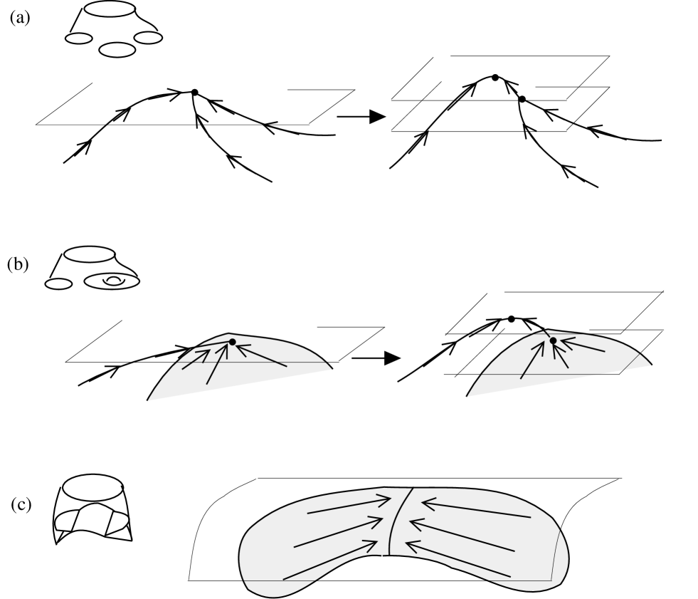
FIG. 4.: (a) and (b) are the examples of the branching crease set in an accidental timeslicing. They are understood by a small deformation of the timeslicing. On the other hand, (c) is the case in which the timeslicing is partially tangent to the crease set. The two-dimensional crease set behaves as a one-dimensional crease set.

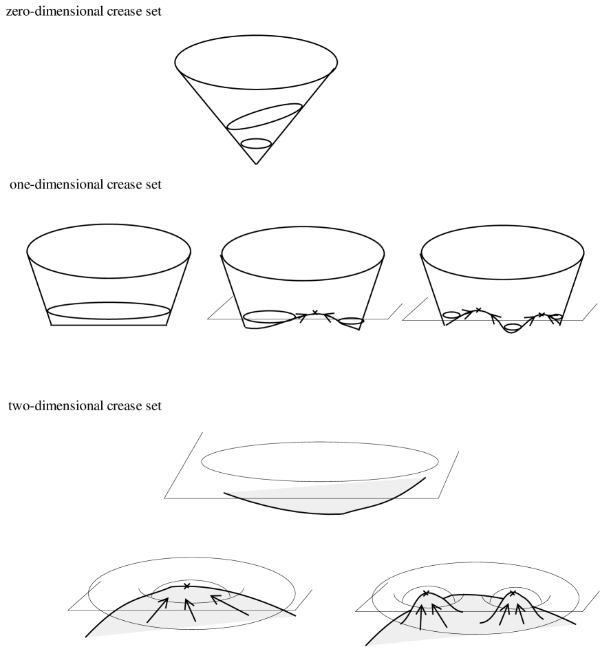
FIG. 5.: EHs with the zero-, one- and two-dimensional crease sets are shown. We see that the one-dimensional crease set becomes a coalescence of an arbitrary number of spherical EHs. For the two-dimensional crease set, only sections of the EH and the crease set are drawn. It can become an EH with an arbitrary number of handles. It is also possible to change the EH into a trivial creation of a spherical EH.

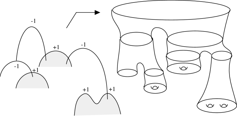
FIG. 6.: An example of the graph of the crease set is drawn. Determining the order of the vertices, we see the TOEH from the index of each zero.

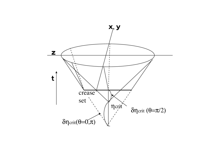
FIG. 7.: The latest light paths with maximal $\delta\eta_{crit}$ ($x,y$ direction in this figure) form an endpoint at the origin with $\eta=\eta_{crit}+\delta\eta_{crit}(\theta=\pi/2)$. On the other hand, a light path on the other axis ($z$-axis in this figure) crosses light paths from other directions and forms an endpoint there. Thus the crease set comes to possess a dimension in this ($z$-)direction.

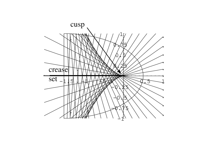
FIG. 8.: The light paths for the elliptic wave front with $a=2,b=1$. There are crossing points of the light paths which are the endpoints of a null surface corresponding to the wave front, on the $x$-axis, $[2x_{0},0]$. A cusp is formed at the origin.

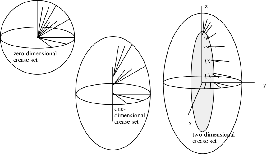
FIG. 9.: The crease set becomes zero-dimensional for the spherical wave front. In the prolate-spheroidal wave front, a one-dimensional crease set appears. Otherwise, the ellipsoidal wave front produces a two-dimensional crease set.

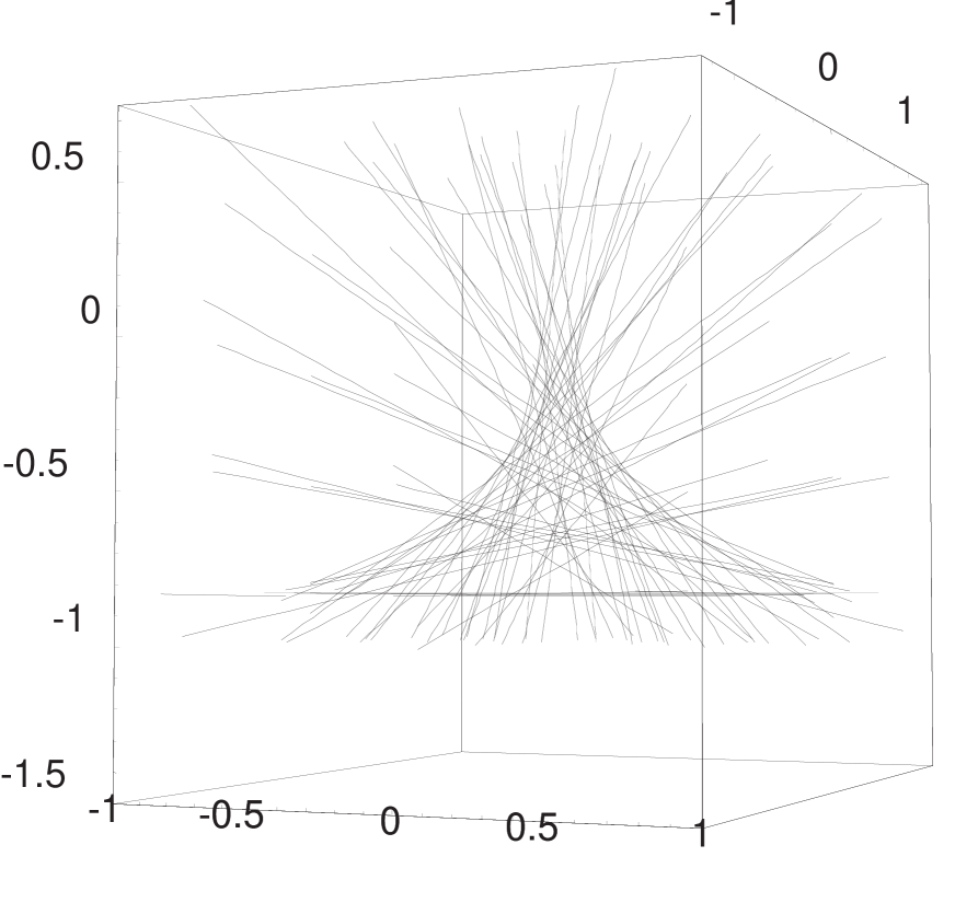
FIG. 10.: The light paths for the ellipsoidal wave front with $a=1,\ b=1.3,\ c=1.5$. A cusp is formed at the origin. Studying this figure carefully, one sees that another cusp exists at $(0,0,(b^{2}-a^{2})/c)$.

FIG. 11.: The EH of the KT solution. It can be seen that the two EHs prior to their coalescence are not smooth at the crease set of the EH.

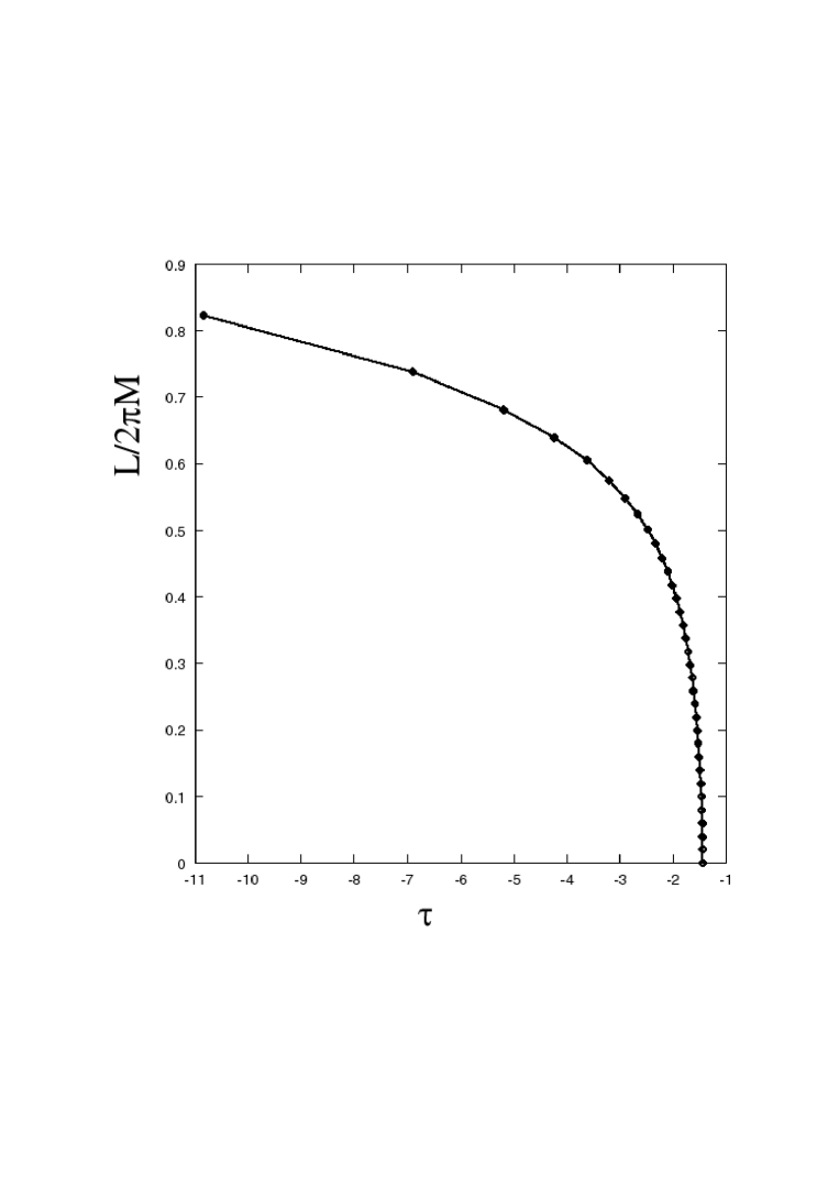
FIG. 12.: The time $\tau$ dependence of the length of the crease set curve later than the time $\tau$. It seems that the length converges to $2\pi M$ as $\tau$ goes to $-\infty$.

FIG. 13.: The EH of the KT solution and a timeslicing. With this timeslicing the EH is regarded as one highly distorted black hole. It is surrounded by a hoop (drawn by a bold curve) whose circumference is $4\pi M$.

REFERENCES

- [1] S. W. Hawking, Commun. Math. Phys. 25 (1972)152.
- [2] S. A. Hughes, C. R. Keeton, P. Walker, K. Walsh, S. L. Shapiro and S. A. Teukolsky, Phys. Rev. D49 (1994)4004, A. M. Abrahams, G. B. Cook, S. L. Shapiro and S. A. Teukolsky Phys. Rev. D49 (1994)5153, S. L. Shapiro, S. A. Teukolsky and J. Winicour Phys. Rev. D52 (1995)6982.
- [3] M. Siino, gr-qc/9701003
- [4] M. Siino, gr-qc/9709015
- [5] D. Ida, K. Nakao, M. Siino and S. Hayward, in preparation.
- [6] P. T. Chrusciel and R. M. Wald, Class. Quant. Grav. 11(1994)L147.
- [7] D. Gannon,Gen. Relativ. Gravit. 7 (1976)219.
- [8] J. L. Friedmann, K. Schleich and D. M. Witt, Phys. Rev. Lett. 71 (1993)1486.
- [9] T. Jacobson and S. Venkataramani, Class. Quantum Grav. 12 (1995)1055.
- [10] S. Browdy and G. J. Galloway, J. Math. Phys. 36 (1995)4952.
- [11] P. Anninos, D. Bernstein, S, Brandt, J. Libson, J. Massó, E. Seidel, L. Smarr, W. Suen, and P. WalkerPhys. Rev. Lett. 74 (1995)630.
- [12] R. M. Wald, General Relativity University of Chicago Press, Chicago, 1984.
- [13] R. D. Sorkin, Phys. Rev. D33 (1985)978.
- [14] R. P. Geroch, J. Math. Phys. 8 (1967)782.
- [15] J. Beem and A. Królak, gr-qc/9709046.
- [16] S. W. Hawking and G. F. R. Ellice, The large scale structure of space-time Cambridge University Press, New York, 1973.
- [17] P. T. Chruściel and G. J. Galloway, gr-qc/9611032.
- [18] I. M. Singer and J. A. Thorpe, Lecture Notes on Elementary Topology and Geometry Springer Verlag, 1976.
- [19] K.S.Thorne, in Magic Without Magic; John Archibald Wheeler, Edited by J.Klauder (Freeman, San Francisco, 1972).
- [20] S. Chandrasekhar, The mathematical theory of black holes, Oxford University Press Inc., New York, 1983.
- [21] S. W. Hawking,Comm. Math. Phys. 43 (1975)199.
- [22] U.H. Gerlach and U. K. Sengupta, Phys. Rev. D19 (1979)2268.
- [23] T. Poston and I. Stewart, Catastrophe theory and its applications, Pitman Publishing Limited, 1978.
- [24] V. I. Arnold, Catastrophe theory, Springer Verlag, 1986.
- [25] K. S. Thorne, in Magic Without Magic; John Archibald Wheeler, Edited by J.Klauder (Freeman, San Francisco, 1972), p.231.
- [26] T. Chiba and K. Maeda, Phys. Rev. D50, 4903 (1994).
- [27] D. R. Brill, G. T. Horowitz, D. Kastor and J. Traschen, Phys.Rev.D49, 840 (1994).
- [28] K. Nakao, T. Shiromizu, and S. A. Hayward, Phys. Rev.D52, 796 (1995).
- [29] D.R.Brill and S.A.Hayward, Class. Quantum Grav.11, 359 (1994).
- [30] M. Seriu, Phys. Lett. B319 (1993)74.
- [31] E.Flanagan, Phys. Rev. D44, 2409 (1991).
- [32] R. Schoen and S. T. Yau,it Commun. Math. Phys. 90 (1983) 575.