Does loop quantum gravity imply $\Lambda=0$?

Abstract

We suggest that in a recently proposed framework for quantum gravity, where Vassiliev invariants span the the space of states, the latter is dramatically reduced if one has a non-vanishing cosmological constant. This naturally suggests that the initial state of the universe should have been one with $\Lambda=0$.

For a long time the problem of the value of the cosmological constant has been viewed as an important open issue in cosmology. The observed value of the constant is quite low (smaller than $10^{-120}$ in Planck units), and most field-theoretic mechanisms for generation of a cosmological constant predict a much higher value. Although one can set the constant to zero by hand, this amounts to a highly artificial fine-tuning. It has therefore been viewed as desirable to find a fundamental mechanism that could set its value to either zero or a very small value. Quantum gravity has been suggested in the past as a possible mechanism. The original proposal is due to Coleman [1], and a recent attractive revision of this proposal was introduced by Carlip [2]. In both proposals the discussion was made at the level of the path integral formulation of quantum gravity. There have also been proposals for “screening” of the cosmological constant in perturbative approaches to quantum gravity [3]. Here we would like to suggest that similar conclusions can be reached when constructing the canonical quantum theory of general relativity.

Canonical quantum gravity was considered for a long time as an intellectual wasteland. The complexity of the constraint equations barred the implementation of even the earlier steps of a canonical quantization program. This made the status whole canonical approach look quite naive, since it could not even begin to grasp with the physics of quantum gravity. The general situation of the canonical approach to quantum gravity started to get better with the introduction of the Ashtekar new variables [4]; but still important difficulties remain before a canonical quantization can be completed. More specifically, the issues of observables and the “problem of time” are still important obstacles to the completion of the canonical quantization program. In spite of this, it has become recently clear that one is in fact able to make use of the formalism to come up with interesting physical predictions, in spite of it being incomplete. This is perhaps better displayed by the recent calculations of black hole entropy [5, 6, 7, 8], which yield physical predictions in spite of not addressing the issues mentioned above. The intention of this note is to show that one can, within the canonical approach, reach certain conclusions about the value of the cosmological constant, again without having a complete formalism. Contrary to the arguments about black hole entropy, those that involve the cosmological constant require, as we will see, a somewhat detailed use of the dynamics of the theory, namely the Hamiltonian constraint. Unfortunately, although progress towards a consistent and physically meaningful definition of the quantum Hamiltonian constraint exists, the issue is not still settled. Our calculations can therefore only be considered as preliminary. We will make use of a recently introduced formulation of the Hamiltonian constraint, that although appealing, has not yet been proved to be completely consistent, especially at the level of the constraint algebra.

Since the early days of the Ashtekar formulation, it became apparent that the Hamiltonian constraint could be written in terms of a differential operator in loop space called the loop derivative [9, 10]. Writing the constraint in this way allowed to operate explicitly on functions of loops and several solutions related to knot invariants were found [13, 11, 12, 14] at a formal level. This early work suffered from several drawbacks. On one hand, it was difficult to consider functions of loops that were compatible with the complicated Mandelstam identities [15] in loop space. Moreover, the loop derivative was not really well defined if the wavefunctions were invariant under diffeomorphisms, which is the case of interest in quantum gravity. Finally, the Hamiltonian was regularized using a background metric, which complicated reproducing the classical Poisson algebra of constraints [16]. A recent series of results have improved the situation regarding some of these issues. By working in the language of spin networks, one is able to do away with the problem of the Mandelstam identities [17]. Moreover, a well defined prescription for the action of the loop derivative can be found [18], and the knot polynomials that were formal solutions can be constructed [19] generalizing earlier work of Witten and Martin [20], and actually found to be solutions of the constraints [18]. More precisely, it was found [18, 21], that the knot invariants that are loop differentiable are Vassiliev invariants, and in particular that the Vassiliev invariants that arise from Chern–Simons theory are a natural “arena” for the discussion of quantum gravity. An intuitive way of understanding this is the fact that this set of invariants is conjectured to separate all knots, and therefore is a natural basis in the space of diffeomorphism invariant functions of loops.

We want here to discuss the construction of solutions with a cosmological constant. We will assume our solutions to be of the form,

$$\Psi(\Gamma)=\sum_{n=p}^{\infty}v_{n}(\Gamma)\Lambda^{n-p},\qquad p>0$$ (1)

where $\Gamma$ is a spin network, $v$’s are Vassiliev invariants. We have assumed here that solutions do not have essential singularities in terms of $\Lambda$ (they could have negative powers of $\Lambda$ and one could reach the above expression by multiplying the wavefunction times the appropriate powers of $\Lambda$). It can be straightforwardly seen that $v_{n}(\Gamma)$ is actually a Vassiliev invariant of order $n$. To see this, one should note that we are interested in finding states that are annihilated by the Hamiltonian constraint,

$$H_{\Lambda}=H_{0}+\Lambda{\rm det}g$$ (2)

where $H_{0}$ is the vacuum (no cosmological constant) Hamiltonian and the other term is proportional to the determinant of the three metric. The quantum action of these operators [18] is such that $\hat{H}_{0}$ acting on a Vassiliev invariant of order $n$ produces one of order $n-1$ and $\widehat{{\rm det}g}$ does not change the order of the invariant it acts upon. Therefore the only chance of cancellations to occur is if $v_{n}$ is an invariant of definite order, $n$.

It is straightforward to see from the above construction, taking the limit $\Lambda\rightarrow 0$, that the leading term in each of the expansions (1), $v_{p}$, has to be a solution to the Hamiltonian constraint without cosmological constant, $\hat{H}_{0}$. In particular, this reinforces the previous point. We know that solutions of the Hamiltonian without cosmological constant are Vassiliev invariants of a given order [18]. We therefore have that per each solution without cosmological constant, we could construct one solution with cosmological constant via the above procedure, i.e. constructing a recurrence relation,

$$\hat{H}_{0}v_{n}=\widehat{{\rm det}g}v_{n-1}.$$ (3)

Up to here, therefore, it appears there are no less states with cosmological constant than without, in fact, the number appears to be the same. However, we have omitted an important requirement of these quantum states, namely that they be diffeomorphism invariants. Vassiliev invariants are diffeomorphism invariant functions of loops, with the exception of the first order invariant $v_{1}$, which is framing-dependent (it is closely related to the self-linking number of a loop). That is, it is an invariant that changes its values when one eliminates a twist from the loop, very much as if it were an invariant of a ribbon rather than of a loop. In the above construction, when $\hat{H}_{0}$ acts on a $v_{n}$ it will generically produce as a result an invariant of order $n-1$ that involves sums of products of primitive Vassiliev invariants of all lower orders, including $v_{1}$ (for reasons of brevity, we omit the detailed calculations here, we refer the reader to [18] for details). Therefore the result is not diffeomorphism invariant. We actually know of examples of solutions like these, constructed by considering the loop transform of the Chern–Simons state. One example of such solutions is the Kauffman bracket knot polynomial, which is of the form (1), but involves $v_{1}$ and powers of it at all orders in the expansion in $\Lambda$.

Therefore, if we wish to require that the resulting wavefunction be diffeomorphism invariant, this will place restrictions on our constructing procedure. This is illustrated in figure 1. The figure represents pictorially by a horizontal line the set of all Vassiliev invariants of a given order. The solid line represents those that are constructed not involving $v_{1}$ and the dashed line those that do. The figure is roughly up to scale, the fraction of invariants that does not depend on $v_{1}$ depends on the number of new primitive Vassiliev invariants that appear at each order. This number is not known precisely, but it is conjectured to grow exponentially. One can then make an estimate of the fraction of invariants dependent on $v_{1}$ to be at least $1/3$ of all invariants. Consider the lower $n$ examples,

$$V_{1}: \qquad v_{1}$$ (4)

$$V_{2}: \qquad v_{1}^{2},v_{2}$$ (5)

$$V_{3}: \qquad v_{1}^{3},v_{2}v_{1},v_{3}$$ (6)

$$V_{4}: \qquad v^{(1)}_{4},v^{(2)}_{4},v_{3}v_{1},v_{2}v_{1}^{2},v_{2}^{2},v_{1}^{4},$$ (7)

the superscripts on $v_{4}$ denote that there are more than one primitive Vassiliev invariants of order four.

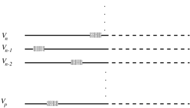
FIG. 1.: The restrictions that occur at each order of recurrence when one requires diffeomorphism invariance.

Now, when the Hamiltonian acts on elements of level $V_{n}$ that do not contain $v_{1}$, it will generically produce an invariant of $V_{n-1}$ that contains $v_{1}$. In this case the original element should be discarded as a potential candidate to generate a diffeomorphism invariant state. The same argument repeats itself at each level. The end result is that in order for the recursion relation to yield framing independent invariants at all orders, one is requiring a very stringent condition on the initial invariant of the series $v_{p}$. That invariant had, to begin with, to be a solution of the vacuum Hamiltonian $H_{0}$. In addition to that, its has to belong in the diffeo-invariant image of the diffeo-invariant portion of $V_{1}$ through the action of $H_{0}$, and so on for each order. The recursion relation has to “thread the hoops” determined by the shaded areas of figure 1. At the very least this implies that there are less solutions of the Hamiltonian constraint starting at a given order $v_{p}$ with cosmological constant than without, if one imposes diffeomorphism invariance. In fact, it appears there could be significantly less. The solutions of the type (1) cannot be constructed with finite series (it would require $\widehat{\rm detg}$ to vanish on the higher order invariant for all spin networks). Therefore one is imposing an infinite number of additional conditions to be satisfied. One cannot make more precise these arguments, since one is dealing with infinite dimensional spaces, but it appears that the requirement is very stringent. It is a fact that we do not know a single solution satisfying this requirement up to now.

We have therefore shown that it is plausible that the canonical theory of quantum general relativity with cosmological constant includes a significantly smaller number of states than vacuum general relativity. In particular, it could be that there are no solutions with cosmological constant. In the latter case, it clearly would prevent us from having a cosmological constant in nature. Even if some solutions with cosmological constant do exist, the fact that gravity with cosmological constant would represent a smaller portion of “phase space” than vacuum general relativity, would make $\Lambda=0$ a more statistically preferred possibility. This could be relevant in settings in which the cosmological constant is allowed to vary primordially, be it through couplings to matter or via “natural selection” mechanisms like proposed in [22].

It is appropriate to finish by pointing out the weak points of the argument. To begin with, the setting in which we are discussing quantum gravity is not completely established. The Hamiltonian constraint we are considering is the “doubly densitized” constraint, that cannot be easily promoted to a regularization-independent quantum operator. This will inevitably bring problems when one wants to check its quantum Poisson algebra. Although we know a few solutions of this Hamiltonian constraint, there is still a lot to be learnt about its space of solutions, especially in the context of spin networks. To be fair, it is also true that we are not using an enormous amount of detail about the action of the constraint, we basically only need that the action on a Vassiliev invariant of order $n$ give as result invariants of order up to $n-1$ in order to construct the argument. Many candidates for Hamiltonians are expected to exhibit this generic property. For our argument to be turned into a rigorous one, one would need a much better control of the space of solutions in order to introduce some sort of measure to determine “how small” is the space of solutions with cosmological constant. The main purpose of this note was not to provide a rigorous argument, but to suggest that in the context of canonical quantization issues like that of the value of the cosmological constant can be addressed. And that with the better control we are gaining on the theory at this level, might be settled rigorously in the near future.

We wish to thank Laurent Freidel, Jorge Griego and Charles Torre for discussions. This work was supported in part by grants NSF-INT-9406269, NSF-PHY-9423950, research funds of the Pennsylvania State University, the Eberly Family research fund at PSU and PSU’s Office for Minority Faculty development. JP acknowledges support of the Alfred P. Sloan foundation through a fellowship. We acknowledge support of Conicyt (project 49) and PEDECIBA (Uruguay).

REFERENCES

- [1] S. Coleman, Nucl. Phys. 310, 643 (1988).
- [2] S. Carlip, Phys. Rev. Lett. 79, 4071 (1997).
- [3] See R. Abramo, N. Tsamis, R. Woodard astro-ph/9803172 and references therein.
- [4] A. Ashtekar, Phys. Rev. Lett. 57, 2244 (1986); Phys. Rev. D36, 1587 (1987).
- [5] L. Smolin, “The Bekenstein Bound, Topological Quantum Field Theory and Pluralistic Quantum Field Theory”, gr-qc/9508064.
- [6] K. Krasnov, Phys. Rev. D55, 3505 (1997).
- [7] C. Rovelli, Phys. Rev. Lett. 77, 3288 (1996).
- [8] A. Ashtekar, J. Baez, A. Corichi, K. Krasnov, Phys. Rev. Lett. 80, 904 (1998).
- [9] R. Gambini, Phys. Lett. B255, 180 (1991).
- [10] B. Brügmann, J. Pullin, Nucl. Phys. 390, 399 (1993).
- [11] B. Brügmann, R. Gambini, J. Pullin, Nucl. Phys. B385, 587 (1992).
- [12] B. Brügmann, R. Gambini, J. Pullin, Gen. Rel. Grav. 25, 1 (1993).
- [13] B. Brügmann, R. Gambini, J. Pullin, Phys. Rev. Lett. 68, 431 (1992).
- [14] R. Gambini, J. Pullin, in “Knots and quantum gravity”, editor J. Baez, Oxford University Press, Oxford (1993).
- [15] R. Gambini, J. Pullin, “Loops, knots, gauge theories and quantum gravity”, Cambridge University Press (1996).
- [16] R. Gambini, A. Garat, J. Pullin, Int. J. Mod. Phys. D4, 589 (1995).
- [17] C. Rovelli, L. Smolin, Nucl. Phys. B442, 593 (1995).
- [18] R. Gambini, J. Griego, J. Pullin, q-alg/9711014, to appear in Phys. Lett. B.
- [19] R. Gambini, J. Griego, J. Pullin, Phys. Lett. B413, 260 (1997).
- [20] E. Witten, Nuc. Phys. B322, 629 (1989); S. Martin, Nuc. Phys. B338, 244 (1990).
- [21] L. Freidel, R. Gambini, J. Pullin, in preparation.
- [22] L. Smolin, “The life of the cosmos”, Oxford University Press, (1987).