Relativistic Hydrodynamics around Black Holes and Horizon Adapted Coordinate Systems

Abstract

Despite the fact that the Schwarzschild and Kerr solutions for the Einstein equations, when written in standard Schwarzschild and Boyer-Lindquist coordinates, present coordinate singularities, all numerical studies of accretion flows onto collapsed objects have been widely using them over the years. This approach introduces conceptual and practical complications in places where a smooth solution should be guaranteed, i.e., at the gravitational radius. In the present paper, we propose an alternative way of solving the general relativistic hydrodynamic equations in background (fixed) black hole spacetimes. We identify classes of coordinates in which the (possibly rotating) black hole metric is free of coordinate singularities at the horizon, independent of time, and admits a spacelike decomposition. In the spherically symmetric, non-rotating case, we re-derive exact solutions for dust and perfect fluid accretion in Eddington-Finkelstein coordinates, and compare with numerical hydrodynamic integrations. We perform representative axisymmetric computations. These demonstrations suggest that the use of those coordinate systems carries significant improvements over the standard approach, especially for higher dimensional studies.

I Introduction

It is well known that the black hole solutions of the field equations of general relativity, with the Schwarzschild and Kerr solutions being astrophysically the most relevant, exhibit coordinate singularities when written in coordinates adapted to the exterior region. The very notion of a black hole was greatly clarified with the discovery, in the early sixties, of coordinate systems that remove those singularities, and indeed cover the whole spacetime [1] (for a general overview see [2],[3]). The (rotating) black hole solution for the metric tensor, expressed in standard Boyer-Lindquist coordinates $(t,r,\theta,\phi)$ is singular at the roots of the equation $\Delta=r^{2}-2Mr+a^{2}=0$ (where $M$ is the mass and $a$ the angular momentum aspect of the hole [4]). In the spherically symmetric Schwarzschild case, the singularity at $r=2M$ is removable with the use of appropriate transformations of the radial and time coordinates. Slightly more complicated transformations, involving also the azimuthal coordinate, can remove the singularities at $r=r_{\pm}=M\pm(M^{2}-a^{2})^{1/2}$ of a rotating black hole.

The location of the coordinate singularity coincides with the event horizon of the black hole. Asymptotic observers lose causal contact with events near the black hole at precisely this location. Hence, despite the singular appearance of the metric, in simulations of matter flows in the background gravitational field of a black hole, one is in principle allowed to consider the open interval extending from the event horizon to some “far zone” at a large, but finite, distance from the hole. This approach has been widely used over the years in the numerical simulations of flows around black holes [5] -[12].

The blow-up of the metric components at the horizon has implications on the behavior of hydrodynamical quantities. The coordinate flow velocity becomes ultra-relativistic and reaches the speed of light at the horizon. As a consequence, the Lorentz factor becomes infinite causing any numerical code to crash. Placing the inner boundary close to the horizon, required for capturing the effects of the relativistic potential, introduces large gradients in all hydrodynamical variables. The steep radial behavior makes the task of numerical evolution with a reasonable degree of accuracy challenging.

Besides practical considerations, the approach of evolving only the exterior domain lacks of a well defined location for the inner boundary: the computation cannot include the horizon surface, but must commence at a location “sufficiently close” to it. Physically, the influence of the horizon region on the solution will progressively red-shift away the closer one gets to the horizon. The validity of a certain choice though, must be continuously reasserted, as new flows or effects are being investigated, with careful tests of convergence, as the inner boundary is progressively moved inwards. Such tests are complicated by the fact that, as mentioned in the previous paragraph, the solutions appear singular at the horizon and hence demand increasingly more resolution.

Ameliorating those problems has motivated the use of a logarithmic radial coordinate (the so-called tortoise coordinate [13]). This technique relegates the event horizon to a infinite, negative, coordinate distance. An equidistant grid in the tortoise $r_{*}$ coordinate maps into an increasingly dense grid in the Schwarzschild $r$ coordinate, with infinite density at the horizon. This approach has proven successful in the extensive semi-analytic studies of black hole perturbation theory, and recently also for the axisymmetric integration of curvature perturbations as an initial value problem [14]. In wave systems, the ambiguity of the location of the inner boundary is addressed by the simple limiting form of the governing equations near the horizon. This is the well known fact that black holes act as finite potential barriers to electromagnetic and gravitational perturbations [15].

The use of a tortoise coordinate does not bring similarly extensive benefits to the study of the hydrodynamical equations. The issue of the inner boundary location is less transparent for those equations. The steepness of the solution and the “artificially” high coordinate velocities persist, although they are now more treatable due to the substantial increase in resolution. In three dimensional simulations using Cartesian coordinates, the tortoise technique is not possible at all. It has been shown recently [16] that adaptive mesh refinement can indeed provide, even for 3D systems, the required resolution close to the event horizon. However, as alluded to above, these undesired pathologies can be eliminated in the case of fixed given black hole backgrounds with rather simple coordinate transformations. This reserves the power of adaptive mesh refinement for the more physically interesting features of the solution.

There is considerable freedom in choosing coordinates regular at the horizon, which can be productively reduced by imposing criteria that can enhance their suitability for numerical applications. The obvious first criterion is of course the regularity of the metric, in particular at the horizon. A second condition is that the constant time surfaces are everywhere spacelike, as this is, currently, a pre-requisite for the implementation of modern numerical methods for relativistic hydrodynamic flows. An important third criterion is the time-independence of the metric components. This leads to constant in time coefficients in the equations and simplifies disentangling the true hydrodynamical evolution from coordinate effects in the black hole background. Interestingly, we will see that those conditions still do not fix the coordinate system uniquely. We show that the number of available choices greatly reduces, but is still infinite, in the rotating black hole case. We give several examples of such systems, which we collectively call horizon adapted coordinate systems.

Such coordinate systems address the issues raised above in a straight-forward way: any radius inside the horizon is equally appropriate (in the idealized continuum limit) for the imposition of a boundary condition, as the domain is causally disconnected from the exterior. Importantly, the irrelevance of the inner boundary location will persist even after the inclusion of other possible local physical processes that may be considered in conjuction with the hydrodynamical flow, e.g., radiative processes. The coordinate velocities of the flow will be bounded at the horizon, as they represent projections of the (finite) fluid four velocity onto a regular coordinate system. Hence the hydrodynamical nature of the flow becomes considerably less demanding on the integration algorithm. Gradients in the solution for scalar variables such as pressure and enthalpy will of course persist. Those are physical and due to the curvature of the black hole, which requires a significant dynamic range for its resolution.

The organization of this paper is as follows. In section II we introduce a class of horizon adapted coordinate systems for a non-rotating black hole. The rotating black hole and the more restricted class of coordinates available in that case are discussed in the Appendix. We outline the numerical hydrodynamical framework of our computations in section III. Exact solutions for spherical (Bondi) accretion are presented in section IV for both dust and perfect fluids. Section V describes the numerical results. In our numerical simulations we focus mainly on the spherically symmetric case, which captures the essential nature of the problem. Some axisymmetric computations are also briefly considered. The coordinate system on which we base our computations is the celebrated Eddington-Finkelstein coordinate system [17],[18].

Our main aim in this report is to show the functionality of this class of coordinate systems as frameworks for the integration of the equations of relativistic hydrodynamics in black hole spacetimes. In three-dimensions (and rotating holes) computations of accretion onto black holes are likely to benefit significantly by the adoption of a horizon adapted coordinate system.

II Horizon adapted coordinate systems

A transformation of the Schwarzschild time $t$ coordinate to a new “generic” coordinate $\hat{t}$ according to

$$d\hat{t}=dt\pm\frac{1}{A(r)}\left(1-G(r)A(r)\right)^{1/2}dr,$$ (1)

where $A(r)=1-2M/r$, and $G(r)$ an arbitrary function, brings the Schwarzschild metric into the form

$$ds^{2}=-A(r)d\hat{t}^{2}\pm 2\left(1-G(r)A(r)\right)^{1/2}d\hat{t}dr+G(r)dr^{2}+r^{2}(d\theta^{2}+\sin^{2}\theta d\phi^{2}).$$ (2)

The four-dimensional metric is next split following the $\{3+1\}$ framework, as

$$ds^{2}=-(\alpha d\hat{t})^{2}+\gamma_{ij}(dx^{i}+\beta^{i}d\hat{t})(dx^{j}+\beta^{j}d\hat{t})$$ (3)

and hence into the lapse function $\alpha=G(r)^{-1/2}$, the shift vector $\beta_{i}=(\pm\left(1-G(r)A(r)\right)^{1/2},0,0)$ or $\beta^{i}=\gamma^{ij}\beta_{j}$, and the intrinsic spatial metric of the constant $\hat{t}$ hypersurfaces $\gamma_{ij}=\mbox{diag}(G(r),r^{2},r^{2}\sin^{2}\theta)$.

We proceed to establish the features we stated above as defining the horizon adapted coordinate systems. The spacelike nature of the foliation is evident for any positive definite function $G(r)$, the normal to the hypersurface given by $n^{\mu}=(G(r)^{1/2},\mp G(r)^{-1/2}(1-G(r)A(r))^{1/2},0,0)$. The independence of all metric functions from the time coordinate $\hat{t}$ is also manifest. The regularity of the metric is also guaranteed if $G(r)$ is bounded from above (we allow exceptions at the true curvature singularities). Hence a large class of horizon adapted coordinates is parametrized by the positive bounded functions $G(r)$. The essential action of the coordinate transformation (1) is to introduce a non-diagonal $g_{tr}$ term (a radial shift vector). The shift covector will always have $\beta_{r}=\pm 1$ at the horizon and the time flow vector ($t^{\mu}=\alpha n^{\mu}+\beta^{\mu}$) will be lightlike there.

The choice of sign in the above formulae affects whether it is the past (-) or future (+) component of the event horizon that is regularized with the coordinate transformations. Some obvious choices for $G(r)$ are $G(r)=1$, $G(r)=(1+2M/r)$, $G(r)=(1+2M/r)(1+(2M/r)^{2})$, etc. The second choice leads to the well known Eddington-Finkelstein (EF) coordinates which we will adopt for the numerical work in this paper. The coordinate transformation (1) and the relevant discussion of regularity is easily generalized for a rotating black hole. As shown in the Appendix, in that case additional conditions of regularity on an off-diagonal spatial metric component considerably reduce the class of horizon adapted coordinates. Further discussion of special cases is given there. Simulations of accretion flows onto rotating black holes in horizon adapted coordinates, more specifically in the Kerr-Schild coordinate system, will be presented elsewhere [19]. We concentrate now on the EF form of the metric, regularizing the future component of the event horizon, which we will use for our hydrodynamical evolutions. With $G(r)=(1+2M/r)$ the metric reads

$$ds^{2}=-\left(1-\frac{2M}{r}\right)d\hat{t}^{2}+\frac{4M}{r}d\hat{t}dr+\left(1+\frac{2M}{r}\right)dr^{2}+r^{2}(d\theta^{2}+\sin^{2}\theta d\phi^{2}),$$ (4)

and correspondingly $\alpha=(\frac{r}{r+2M})^{1/2}$, $\beta_{r}=\left(2M/r\right)$ and $\gamma_{ij}=\mbox{diag}(1+2M/r,r^{2},r^{2}\sin^{2}\theta)$.

The EF form of the metric represents an analytic extension of the Schwarzschild solution from the region $2M<r<\infty$ to $0<r<\infty$. It is among the algebraically simplest choices and generalizes to the case of a rotating black hole. In three dimensions it is naturally expressed in pseudo-Cartesian coordinates (Kerr-Shild form). An important coordinate property of the EF system is its adaptation to the null cone structure of the black hole: the ingoing radial null geodesics are described in a particularly simple way.

Recent work clearly indicates that coordinate systems regular at the horizon, adapted to the local light cone structure, carry considerable advantages for the evolution of generic black holes. More specifically, the EF system and its generalization for dynamic spherically symmetric spacetimes has been used, for the integration of a self gravitating scalar field in interaction with a black hole [20]. In three dimensional integrations of the Einstein equations, the stable evolution of an isolated black hole has been an important target in the field of numerical relativity. The EF coordinates have been identified [21] as a point of departure for such integrations of the Cauchy problem. Recently, the Binary Black Hole Grand Challenge Alliance project demonstrated [22] the first advection of a black hole in a three-dimensional computational grid using the EF framework in boosted form. More remarkably, “eternal” evolutions have been achieved [23] using a formulation of the Einstein equations based on ingoing characteristic foliations.

Those features of the EF family of coordinate systems do not appear particularly relevant for hydrodynamical computations, since generic fluid flows are not tied to the spacetime null-cone structure in any essential way. It is apparent though, that in simulations accounting for the bidirectional coupling of matter to the spacetime geometry, computations of black hole interactions with matter would benefit significantly from this framework. This motivation breaks the degeneracy among coordinate systems for our purposes.

III Relativistic hydrodynamics and Numerical method

To demonstrate the feasibility of the procedure for numerical studies, we compute the hydrodynamic accretion of fluid flows onto black holes in the EF coordinate system. To do this, we solve the general relativistic hydrodynamic equations in these particular coordinates. Recently, Banyuls et al. [11] have written these equations as an explicit hyperbolic system of conservation laws (with sources) for a general metric written in $\{3+1\}$ form. Here, we have to specialize those general expressions to the metric given by Eq. (4). The evolved quantities are the relativistic densities of particle number, $D$, momentum (in the $i$ direction), $S_{i}$ and energy, $\tau$. These quantities are defined in terms of a set of primitive variables $(\rho,v_{i},\epsilon)$ as $D=\rho W$, $S_{i}=\rho hW^{2}v_{i}$ and $\tau=\rho hW^{2}-p-D$. Here, $\rho$ is the rest-mass density, $p$ is the pressure, $v_{i}$ is the 3-velocity of the fluid and $h$ is the specific enthalpy, defined as $h=1+\epsilon+p/\rho$, with $\epsilon$ being the specific internal energy.

The contravariant components of the 3-velocity are defined as

$$v^{i}=\frac{u^{i}}{\alpha u^{t}}+\frac{\beta^{i}}{\alpha},$$ (5)

where $u^{\mu}$ is the fluid 4-velocity, $\alpha$ is the lapse function ($\alpha^{2}=-1/g^{tt}$). Indices for spatial vectors (the shift vector and the 3-velocity) are raised and lowered using the spatial part of the metric, $\gamma_{ij}$. The quantity $\alpha u^{t}$ is the Lorentz factor, $W$, which satisfies $W=(1-v^{2})^{-1/2}$ with $v^{2}=\gamma_{ij}v^{i}v^{j}$.

We have written a numerical code to solve the general relativistic hydrodynamic equations in the background spacetime of a non-rotating hole, using the EF coordinates. For this purpose we have taken advantage of the fact that the equations form a hyperbolic system and are explicitely written in conservation form [11]. This allows for the use of advanced numerical methods based on approximate (linearized) Riemann solvers whose improved ability to handle relativistic (and ultrarelativistic) flows, high Mach number flows and discontinuous solutions (shock waves), have been recently investigated (see, e.g, [11],[12], [24] and references therein). The Riemann solver used (either Roe [25] or Marquina [26], [27]) relies on the spectral decomposition of the Jacobian matrices of the multidimensional system of relativistic equations. The spatial accuracy of the code is improved by means of a monotonic piecewise-linear reconstruction [28] of proper rest-mass density, flow velocity and internal energy. Integration in time is done using a total-variation-diminishing Runge-Kutta scheme of high-order, developed by Shu and Osher [29] We refer the interested reader to [11] and [30] for further details on the system of equations and the numerical code.

IV Exact solutions

The feasibility of the procedure is shown with a comparison of the numerical integration with exact solutions for spherically symmetric accretion of dust and perfect fluid. Here, we re-derive those exact solutions in the EF coordinate system.

Following Michel [31] we integrate the steady-state hydrodynamic equations to obtain

$$\sqrt{-g}\rho u^{r}=C_{1},$$ (6)

$$\sqrt{-g}\rho u^{r}u_{t}=C_{2},$$ (7)

where $C_{1}$ and $C_{2}$ are integration constants and $g$ stands for the determinant of the four-metric, $\sqrt{-g}=\alpha\sqrt{\gamma}$, with $\gamma=\det{(\gamma_{ij})}$. Hence, $u_{t}=C_{2}/C_{1}=C_{3}$. The coordinate velocity $v^{r}$ is determined by $C_{3}$ and $u_{r}$ through the condition $g_{\mu\nu}u^{\mu}u^{\nu}=-1$.

For the dust case, the final expressions are simple algebraic functions. Fixing $u_{t}=C_{3}=-1$ (the marginally bound case) the solution reads

$$\rho(r)=\frac{-C_{1}}{r^{2}\sqrt{\frac{2M}{r}}},$$ (8)

$$v^{r}(r)=-\frac{1}{\sqrt{1+\frac{r}{2M}}(1+\sqrt{\frac{2M}{r}}+\frac{2M}{r})},$$ (9)

which is valid in the domain $0<r<\infty$, i.e., also inside the horizon. The radial dependence of the rest of the hydrodynamical quantities can be directly computed from these two equations.

Let us turn now to the perfect fluid case. Monotonic steady-state infall of perfect fluid onto a black hole must pass through the critical point of the so-called “wind” equation, obtained by differentiation of the integrated steady state equations (Eqs. (6) and (7)) with respect to $\rho$, $u^{r}$ and $r$, and elimination of the $d\rho$ differential,

$$\frac{du^{r}}{u^{r}}\left[V^{2}-\frac{(u^{r})^{2}}{u_{t}^{2}}\right]+\frac{dr}{r}\left[2V^{2}-\frac{M}{ru_{t}^{2}}\right]=0,$$ (10)

where $V^{2}\equiv\frac{d\ln(\rho h)}{d\ln\rho}-1$ and $u_{t}^{2}=(u^{r})^{2}-g_{tt}$. Using the critical condition, that is, the assumption that both brackets in Eq. (10) vanish simultaneously, the relation $(u^{r}_{c})^{2}=M/2r_{c}$ determines $u^{r}_{c}$ and $(u_{t})_{c}$, after the selection of the critical point radius $r_{c}$. From $u^{r}$ we get $u_{t}$ and hence we obtain $V^{2}$ at the critical radius, $V_{c}^{2}=(u^{r}_{c}/u_{t_{c}})^{2}$. On the other hand, considering a polytropic equation of state $P=K\rho^{\Gamma}$, with adiabatic index $\Gamma$ and a critical density $\rho_{c}$, we can infer the value of $V_{c}^{2}$, which, in conjuction with $V_{c}^{2}=(u^{r}_{c}/u_{t_{c}})^{2}$ determines the polytropic index $K$. This complete determination of the fluid parameters at the critical point, combined with the steady-state conditions, fixes the integration constants $C_{1}$ and $C_{2}$, and hence uniquely identifies the extension of the solution away from the critical point. Contrary to the dust case, the solution does not have a closed form, as one must solve a non-linear algebraic equation for $u^{r}(r)$, from which one can get the rest of the variables. This is done using a Newton-Raphson iteration.

V Results

We now use the exact solutions derived in the previous section to check the accuracy of our numerical evolutions and to demonstrate the feasibility of our approach. For the numerical investigation we consider homogeneous initial data across the domain of integration. The initial data evolve in time, until a final steady-state solution is reached. We focus mainly on the spherically symmetric case, to which the exact solutions apply. At the end of the section we describe some axisymmetric computations.

In spherical symmetry, the numerical domain extends from any given non-zero radius inside the horizon, $r_{min}$, to some $r_{max}$ located in the physical universe (outside the horizon). In Figs. 1 and 2 we plot a comparison of the exact and numerical solutions for the dust and perfect fluid cases, respectively. We show the final steady-state for the spherical accretion problem. The solid lines represent the exact solution and the circles indicate the numerical one. In the particular computations considered here we have chosen $r_{min}=0.5M$ and $r_{max}=50M$. We have used a non-uniform numerical grid of 200 zones (logarithmic spacing). In both the dust and perfect fluid integrations we have only assumed the exact solution in the outermost zone. The integration has been performed until the final steady-state solution has been achieved in the whole domain. The perfect fluid equation of state is given by $p=(\Gamma-1)\rho\epsilon$, with $\Gamma$ being the (constant) adiabatic exponent of the gas. We have chosen $\Gamma=4/3$.

The solutions are seen to be regular well inside the horizon at $r=2M$. Nothing special happens at the horizon where all quantities are smooth. The steepness of the hydrodynamic quantities dominates the solution only near the real singularity. It is worth to stress the behavior of the velocity in this new coordinate system, which differs considerably from the Schwarzschild case. Now the total velocity does not approach the speed of light as it reaches the horizon, and although the maximum fluid speed is still at $r=2M$, it is now considerably smaller, $v=\sqrt{\gamma_{rr}}v^{r}=1/\sqrt{3}$, in the dust case. For the perfect fluid case this value is even smaller, due to the pressure support of the gas. This is a most attractive numerical behavior, as it eliminates the divergence in the Lorentz factor at the horizon which would cause any relativistic fluid dynamics code to crash. As can be deduced from both figures we have found very good agreement with the exact solution. In Fig. (3) we display the relative errors for density, pressure and total velocity in the case of perfect fluid accretion.

The resolution benefits from the use of horizon adapted coordinates appear to be considerable, hence we attempt a rough quantitative assessment. We perform a sequence of comparison integrations in Schwarzschild and EF coordinates. We focus on the case of spherical dust accretion. We use a grid of 100 zones and evolve the stationary solution up to a final time of $100M$. The outer boundary of the domain is fixed at $50M$. The inner boundary of the EF domain is fixed at $1.5M$. For the Schwarzschild computation we use a tortoise radial coordinate which provides very high resolution near the horizon. We have found that the solution in Schwarzschild coordinates is maintained stationary, provided $r_{min}\geq 2.1M$. For $r_{min}=2.05M$ and a maximum resolution of $10^{-3}M$, the accretion departs from the exact initial solution at the zones closer to the horizon. For $r_{min}=2.01$ and same resolution, the code crashes. In this case, a grid of 200 points does not preserve the initial solution either (even with a resolution of $10^{-4}M$). At least 400 zones are required (with a maximum $\Delta r\approx 10^{-5}$) to achieve the correct accretion pattern. On the other hand, using EF coordinates, we can resolve the problem with an (unequally spaced) grid of 50 zones. This gives, broadly speaking, a factor of 8 benefit in resolution when using horizon adapted coordinate systems. Computations that may require small values of $r_{min}$ will further increase this number, the same being true for perfect fluid computations. In this latter case the computation in standard coordinates is more challenging, as the pressure (or the internal energy) can easily become unstable near the horizon and even become negative. Finally, three dimensional Cartesian computations do not allow the use of tortoise coordinate based grids. Hence a conservative estimate introduces an $8^{3}$ gain factor in the size of tractable problems in three dimensional integrations.

We now briefly describe axisymmetric computations. We study the so-called Bondi-Hoyle accretion, that is, hydrodynamic accretion onto a moving black hole, in the EF coordinate system (for a general overview of such flows see, e.g., [12] and references therein). The asymptotic values of fluid velocity, $v_{\infty}$, sound speed, $c_{s_{\infty}}$ and adiabatic exponent, $\Gamma$, together with the assumption of an initially homogeneous distribution suffice to define the initial values of all hydrodynamical quantities. As in the spherical case, these data evolve towards a final steady-state solution. We use a grid of $200\times 100$ zones in $r$ and $\theta$, respectively, with $r_{min}=1.5M$, $r_{max}=100M$ and $0\leq\theta\leq\pi$. The radial grid is logarithmically spaced. We evolve a model with $c_{s_{\infty}}=0.1$, and $v_{\infty}=0.5$. Hence, it is a supersonic model with Mach number $5$. We plot in Fig. 3 the stationary solution for $\Gamma=4/3$ (top), $5/3$ (middle) and $2$ (bottom). We plot iso-contours of the logarithm of the density. The most prominent feature of the solution is the stationary conical shock. The inner circle indicates the position of the horizon. Again, as in the spherical case, the solution smoothly straddles the horizon at $2M$. Compared to the evolutions presented in [12] in Schwarzschild coordinates, we now use less resolution to get to the same final solution. Highly supersonic models with large values of $\Gamma$, in particular $\Gamma=5/3$, were very hard to evolve with Schwarzschild coordinates and the $\Gamma=2$ case was impossible to evolve. Its computation is now straightforward.

VI Conclusions

We have presented a family of horizon adapted coordinate systems for the numerical study of accretion flows around black holes. In the rotating case we identify a discrete but infinite family, of which the first simple members are well known stationary coordinate systems. In the non-rotating case the freedom in building the regular stationary foliation is quantified by (at least) the space of bounded positive functions of one variable. We have shown how these systems allow for a better numerical treatment of accretion scenarios. Existing numerical studies of accretion flows onto black holes have been performed in the original, singular systems, i.e., Schwarzschild coordinates for the Schwarzschild solution and Boyer-Lindquist coordinates for the rotating (Kerr) solution. Although it is possible to solve the problem in these pathological coordinates, one is introducing artificial complexity, being forced to use very high resolution to deal with the unphysically large gradients that develop in the vicinity of the horizon. This may prevent the accurate solution of three dimensional problems. At the same time, the ambiguity regarding the position of the inner boundary of the domain (which should be the horizon) introduces a convergence criterion that must be enforced at all times if the solutions are to be trusted.

We have focussed on the particular case of the Eddington-Finkelstein form of the Schwarzschild metric. The general relativistic hydrodynamic equations are now regular at the horizon, which permits an accurate description of accretion flows. We have demonstrated the feasibility of this approach with the numerical study of the spherical accretion (Bondi accretion) of dust and perfect fluid, and the comparison with the exact solutions which we re-derived in this coordinate system. We have also shown the functionality of the new coordinates in axisymmetric computations of relativistic Bondi-Hoyle accretion flows.

In a forthcoming paper we plan to extend this approach to the rotating case, considering horizon adapted coordinate systems to study accretion flows in stationary Kerr spacetimes. Three dimensional accretion flows onto black holes are interesting both from an astrophysical and geometrical point of view, as they are thought to correspond to observable electromagnetic emission, and hence may help map the relativistic rotating black hole potential. The framework proposed here will help detailed numerical studies of such systems in the near future.

In this appendix we present stationary coordinate systems for the Kerr spacetime that are regular at and outside the horizon $r_{+}$, i.e., the larger of the roots of the equation $\Delta\equiv r^{2}-2Mr+a^{2}=0$. In the Boyer-Lindquist form for the metric tensor the $\gamma_{rr}$ component is singular at $r_{+}$,

$$ds^{2} = -\frac{\Delta}{\rho^{2}}\left[dt-a\sin^{2}\theta d\phi\right]^{2}+\frac{\sin^{2}\theta}{\rho^{2}}\left[(r^{2}+a^{2})d\phi-adt\right]^{2}$$ (12)

$$+\frac{\rho^{2}}{\Delta}dr^{2}+\rho^{2}d\theta^{2},$$

with $\rho^{2}\equiv r^{2}+a^{2}\cos^{2}\theta$. We now introduce a coordinate transformation defined by

$$d\hat{\phi} = d\phi-\frac{a}{\Delta}\epsilon(r,\theta)dr,$$ (13)

$$d\hat{t} = dt-\epsilon(r,\theta)\left[\frac{r^{2}+a^{2}}{\Delta}-\frac{\rho^{2}}{\rho^{2}-2Mr}\left(1-\sqrt{1-\left(1-\frac{2Mr}{\rho^{2}}\right)G(r,\theta)}\right)\right]dr,$$ (14)

where $\epsilon$ and $G$ are, at present, arbitrary functions. This form of the transformation is chosen in order to isolate the singular behavior of the spatial metric. With the above ansatz, the metric becomes, in the new coordinates $(\hat{t},r,\theta,\hat{\phi})$,

$$ds^{2} = -\left(1-\frac{2Mr}{\rho^{2}}\right)d\hat{t}^{2}-\frac{4Mar}{\rho^{2}}\sin^{2}\theta d\hat{t}d\hat{\phi}$$ (18)

$$-2\epsilon\sqrt{1-\left(1-\frac{2Mr}{\rho^{2}}\right)G}d\hat{t}dr+\left[\frac{1-\epsilon^{2}}{\Delta}\rho^{2}+G\right]dr^{2}$$

$$+2\epsilon\frac{a\sin^{2}\theta\rho^{2}}{\rho^{2}-2Mr}\left[1-\frac{2Mr}{\rho^{2}}\sqrt{1-\left(1-\frac{2Mr}{\rho^{2}}\right)G}\right]d\hat{\phi}dr$$

$$+\rho^{2}d\theta^{2}+\sin^{2}\theta\left[\rho^{2}+a^{2}\sin^{2}\theta\left(1+\frac{2Mr}{\rho^{2}}\right)\right]d\hat{\phi}^{2}.$$

By inspection of the spatial metric components we see that the condition of regularity at the $\Delta=0$ surface demands that $\epsilon^{2}=1$. This fixes the function $\epsilon$ up to a sign. We proceed to further examine the regularity of the metric element. All components of the metric, except $\gamma_{r\hat{\phi}}$, are regular, except at the points $\rho^{2}=0$, which belong to the true singularity. The component $\gamma_{r\hat{\phi}}$ is singular at the ergosphere ($\rho^{2}-2Mr=0$) which is outside the $r_{+}$ horizon, and coincides with it at the poles $\theta=0,\pi$.

Before we ameliorate this pathology we note that in the case of no rotation $(a=0)$, the off-diagonal term drops, hence as we have already seen in section (II) there is no restriction on the choice of the function $G$. This special behavior of the Schwarzschild black hole allows selecting $G$ with the target of simplifying the spatial 3-metric. An interesting coordinate system, is obtained with the simple choice $G(r)=1$, which brings the metric into the form

$$ds^{2}=-\left(1-\frac{2M}{r}\right)d\hat{t}^{2}+2\sqrt{\frac{2M}{r}}d\hat{t}dr+dr^{2}+r^{2}(d\theta^{2}+\sin^{2}\theta d\phi^{2}),$$ (19)

and correspondingly $\alpha=1$, $\beta_{r}=\left(2M/r\right)^{1/2}$ and $\gamma_{ij}=\mbox{diag}(1,r^{2},r^{2}\sin^{2}\theta)$. This is the Lemaitre coordinate form of the Schwarzschild solution [32]. The trivial form of the lapse and the three-metric imply that all of the curvature information of the black-hole spacetime is encoded in the way the $r,\theta,\phi$ coordinates must propagate from time slice to time slice (choice of shift vector), in order to preserve a flat 3-space, and a constant rate of clock ticking. It is quite remarkable that such a shift vector is a simple, time-independent, function of radius, which, incidentally, is equal to the Newtonian free fall velocity as measured locally by static observers. This form of the metric element was the starting point for a program of constructing black hole initial data [33]. Unfortunately, this simple state of affairs does not appear generalizable to the rotating case.

Returning to the general case, by further exercising the freedom in choosing the function $G(r,\theta)$ we can ensure that the off-diagonal metric component is regular.

Substituting for $G$ via

$$1-\left(1-\frac{2Mr}{\rho^{2}}\right)G=Z^{2},$$ (20)

we see that the class of regular systems is parametrized by the functions

$$Z_{k}=\left(\frac{2Mr}{\rho^{2}}\right)^{k},$$ (21)

where $k$ is a non-negative integer. The general admissible form for the function $G(r,\theta)$ is

$$G_{k}=1+\frac{2Mr}{\rho^{2}}+\ldots+\left(\frac{2Mr}{\rho^{2}}\right)^{2k-1},$$ (22)

for non-zero $k$, and

$$G_{0}=0.$$ (23)

With those substitutions the metric becomes

$$ds^{2} = -\left(1-\frac{2Mr}{\rho^{2}}\right)d\hat{t}^{2}-\frac{4Mar}{\rho^{2}}\sin^{2}\theta d\hat{t}d\hat{\phi}$$ (26)

$$+\rho^{2}d\theta^{2}+\sin^{2}\theta\left[\rho^{2}+a^{2}\sin^{2}\theta\left(1+\frac{2Mr}{\rho^{2}}\right)\right]d\hat{\phi}^{2}$$

$$-2\epsilon Z_{k}d\hat{t}dr+G_{k}dr^{2}+2\epsilon a\sin^{2}\theta W_{k}d\hat{\phi}dr,$$

where

$$W_{k}=1+\frac{2Mr}{\rho^{2}}+\ldots+\left(\frac{2Mr}{\rho^{2}}\right)^{k},$$ (27)

and all terms are regular except at the true curvature singularity.

The case $k=0$ corresponds to the ingoing and outgoing Eddington-Finkelstein coordinates ($\epsilon=-1$ and $\epsilon=1$ respectively). In this case the coefficient of the $\gamma_{rr}$ vanishes. Despite a common misconception, the foliation is still spacelike [34] for non-zero $a$. The null character of the foliation in the limit $a=0$, though, implies that this coordinate system is not appropriate for $3+1$ based studies.

The case $k=1$ generates the Kerr-Schild coordinate system, expressed in spherical coordinates via the relations [3]

$$x+iy = (r+ia)\sin\theta e^{i\hat{\phi}},$$ (28)

$$z = r\cos\theta.$$ (29)

It is the algebraically simplest member of the family and reduces to the EF system in the $a=0$ case.

The case $k=2$ introduces a time coordinate that satisfies a harmonic condition [35], i.e., $\Box\hat{t}=0$. Some recent hyperbolic formulations of the Einstein equations are based on harmonic slicings, hence the black hole metric expressed in such coordinate systems can be used effectively as a numerical code test-bed [36].

The higher order members of the family, i.e., $k=3,4,\ldots$ may also have interesting geometrical or differential properties.

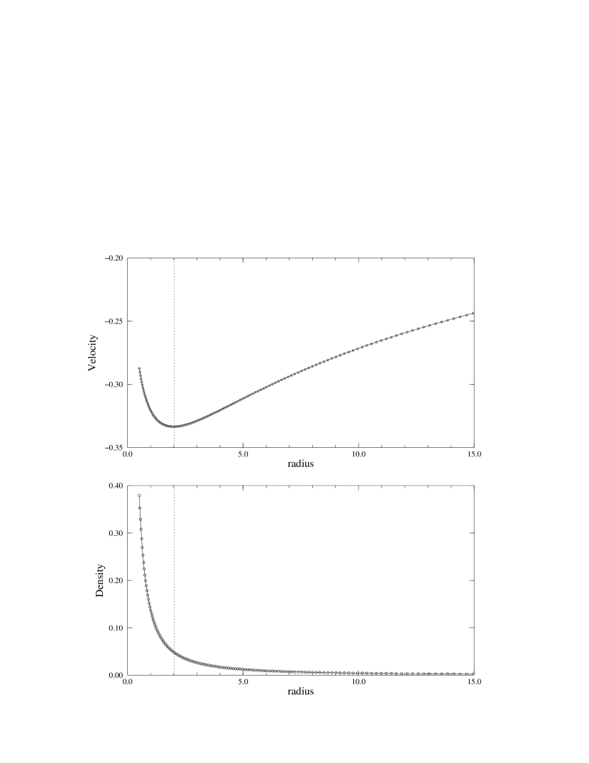
FIG. 1.: Exact (solid line) versus numerical (circles) solution for spherical accretion of dust, after reaching the steady-state. The top curve shows the total velocity and the bottom one shows the rest-mass density, as a function of the radial coordinate. The total domain extends to $50M$. We focus on the first $15M$. The value of $C_{1}$ in Eq. $(\ref{dens})$ was chosen to be $-0.195$. The numerical solution agrees well with the exact one. The dotted line marks the position of the horizon.

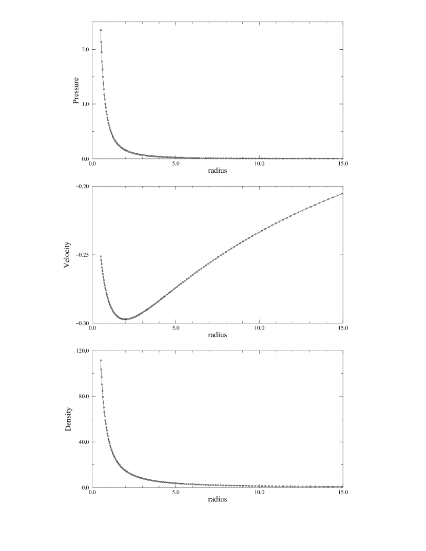
FIG. 2.: Exact (solid line) versus numerical (circles) solution for spherical accretion of a perfect fluid, after reaching the steady-state. The top curve shows the pressure, the middle one shows the total velocity and the bottom one shows the rest-mass density, as a function of the radial coordinate. As in Fig. 1, the total domain extends to $50M$ and we only plot the first $15M$. The numerical and exact solutions also match very well. The dotted line marks the position of the horizon. The critical point values used to construct this particular exact solution are $r_{c}=400M$ and $\rho_{c}=10^{-2}$.

FIG. 3.: Relative errors for density, pressure and total velocity in the case of perfect fluid accretion, as a function of the radial coordinate $r$. The result is for 200 grid points between 0.5 and $50M$. Only the first $15M$ are shown. The overall good accuracy is apparent, the especially small error in total velocity being most striking.

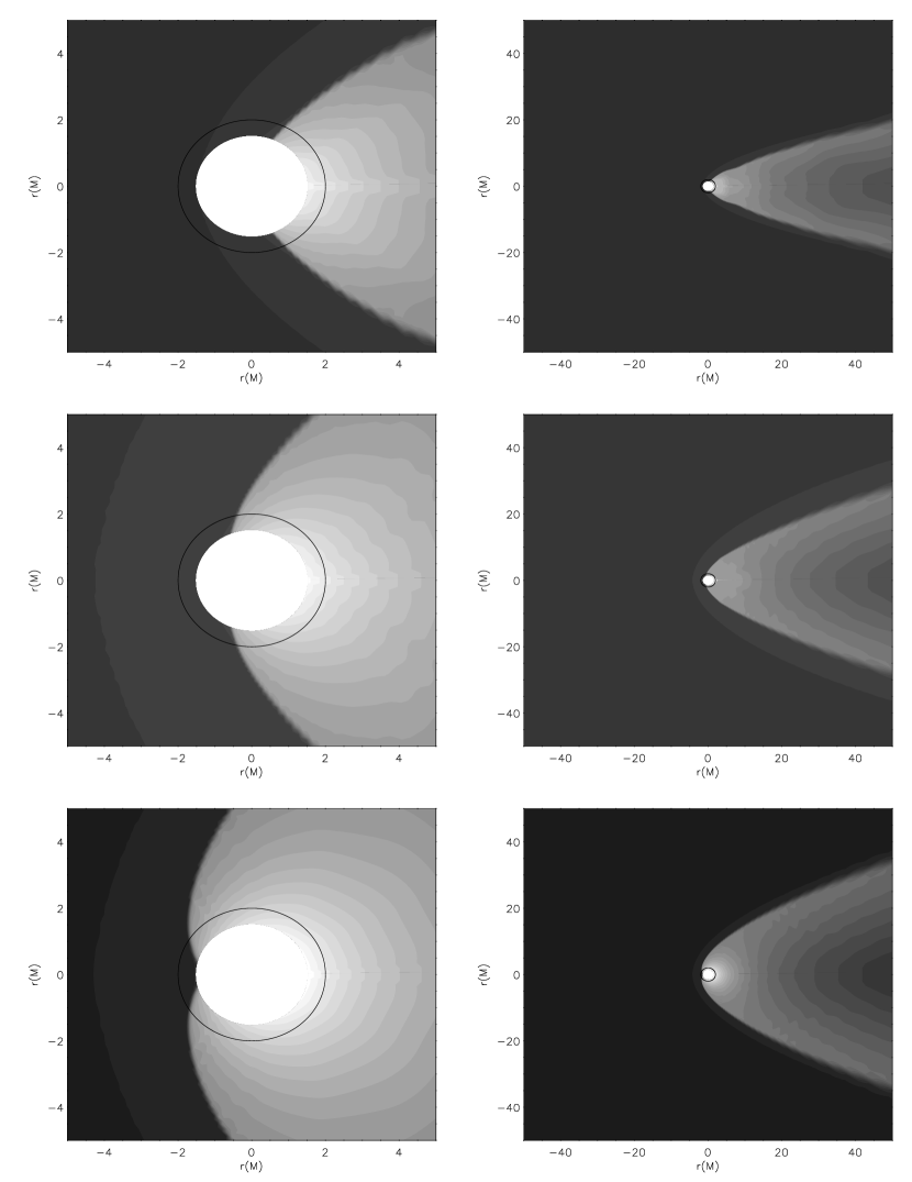
FIG. 4.: Grey-scale iso-contour plots of the logarithm of the rest-mass density for the axisymmetric relativistic Bondi-Hoyle accretion problem. The final stationary solution is plotted. From top to bottom we display the solution for $\Gamma=4/3$, $5/3$ and $2$, respectively. The left column shows a close-up view of the central region, which is enlarged in the right column. The inner circle shows the location of the horizon. The shock cone is well resolved even at large distances from the hole. Its innermost location differs in the three cases. For larger values of $\Gamma$ it moves to the front part of the hole, due to the higher pressure values at its rear part.

REFERENCES

- [1] M.D. Kruskal, Phys. Rev. 119, 1743-1745 (1960).
- [2] C.W. Misner, K.S. Thorne and J.A. Wheeler, Gravitation, W.H. Freeman and Co. (1973)
- [3] S.W. Hawking, and G.F.R. Ellis, The large scale structure of spacetime, Cambridge University Press (1973).
- [4] Geometrized units are used throughout the paper.
- [5] J. R. Wilson, ApJ 173, 431 (1972).
- [6] J.F. Hawley, L.L. Smarr, and J.R. Wilson, ApJ 277, 296 (1984).
- [7] J.F. Hawley, L.L. Smarr, and J.R. Wilson, ApJSS 55, 211 (1984).
- [8] L.I. Petrich, S.L. Shapiro, R.F. Stark, and S.A. Teukolsky, ApJ 336, 313 (1989).
- [9] A.M. Abrahams, and S.L. Shapiro, Phys. Rev. D 41, (2) 327-341 (1990).
- [10] F. Eulderink and G. Mellema, A&ASS 110, 587 (1995).
- [11] F. Banyuls, J.A. Font, J.M. Ibáñez, J.M. Martí, and J.A. Miralles, ApJ 476, 221 (1997).
- [12] J.A. Font and J.M. Ibáñez, ApJ 494, 297 (1998).
- [13] T. Regge and J.A. Wheeler, Phys. Rev. 108, 1063 (1957).
- [14] W. Krivan, P. Laguna, P. Papadopoulos, and N. Andersson, Phys. Rev. D 56, 3395 (1997).
- [15] S. Chandrasekhar, The Mathematical Theory of Black Holes, Oxford University Press (1983).
- [16] P. Papadopoulos, E. Seidel, and L.A. Wild, Phys.Rev.D. (submitted)
- [17] A.S. Eddington, Nature 113, 192 (1924).
- [18] D. Finkelstein, Phys. Rev. 110, 965-967 (1958).
- [19] J.A. Font, J.M Ibáñez, and P. Papadopoulos. (in preparation)
- [20] M. Marsa and Choptuik, Phys.Rev. D 54, 4929 (1996).
- [21] G. Allen et al., in Proceedings of the Seventh Marcel Grossmann Meeting on General Relativity, edited by R.T.Jantzen and G.M.Keiser, (World Scientific, Singapore, 1996), pp.615-618.
- [22] G. Cook et al., Phys. Rev. Lett. (submitted)
- [23] R. Gomez et al., Phys. Rev. Lett. (submitted)
- [24] J.M. Martí, E. Müller, J.A. Font, J.M Ibáñez, and A. Marquina, ApJ 479, 151 (1997).
- [25] P. Roe, J. Comput. Phys. 43, 357 (1981).
- [26] R. Donat,and A. Marquina, J. Comput. Phys. 125, 42 (1996).
- [27] R. Donat, J.A. Font, Ibáñez, J.M. and Marquina, A., J. Comput. Phys. (in press).
- [28] B. van Leer, J. Comput. Phys. 32, 101 (1979).
- [29] C. Shu, and S. Osher, J. Comput. Phys. 77, 439 (1988).
- [30] J.A. Font, J.M. Ibáñez, A. Marquina,and J.M. Martí, A&A 282, 304 (1994).
- [31] F.C. Michel, Ap. Space Sci. 15, 153 (1972).
- [32] G. Lemaitre, Compt. Rend. Acad. Sci. (Paris), 196, 903 (1933).
- [33] D.M. Eardley, in Dynamical Spacetimes and Numerical Relativity, edited by J.M. Centrella (Cambridge University Press, 1985).
- [34] F. Pretorius and W. Israel, (gr-qc/9803080).
- [35] C. Bona and J. Masso, Phys. Rev. D. 38, 2419 (1988).
- [36] G.B. Cook and M.A. Sheel, (BBHGC report).