Neutron star in presence of torsion-dilaton field

Abstract

We develop the general theory of stars in Saa’s model of gravity with propagating torsion and study the basic stationary state of neutron star. Our numerical results show that the torsion force decreases the role of the gravity in the star configuration leading to significant changes in the neutron star masses depending on the equation of state of star matter. The inconsistency of the Saa’s model with Roll-Krotkov-Dicke and Braginsky-Panov experiments is discussed.

PACS number(s): 04.40.Dg,04.40.-b,04.50.+h

1 Introduction

In recent years the interest in scalar-tensor theories of gravity has been renewed. One reason for this is the important role which these theories play in the understanding of inflantionary epoch. On the other hand the scalar-tensor gravitation (the so called ”dilaton gravity”) arises naturally from the low-energy limit of the super-string theory [1], [2].

The predictions of scalar-tensor theories may differ drastically from these of general relativity. For example such a phenomenon – ”spontaneous scalarization” was recently discovered by Damour and Esposito-Farese as a non-perturbative strong field effect in a massive neutron star [3]. Other interesting phenomenon is ”gravitational memory” of black holes proposed in [4]. The ”gravitational memory” in the case of boson stars was investigated in [5] (see also [6]).Their stability through cosmic history using catastrophe theory was investigated in [7].

Many theories of gravity with propagating torsion involving a scalar field have been proposed in the last decades, too [8], [9], [10]. In such theories contrary to the usual Einstein-Cartan gravity [11]-[13], there are long-range torsion mediated interactions. Carrol and Field [14] have examined some observational consequences of propagating torsion in a wide class of models involving a scalar field. They conclude that for reasonable models the torsion could be detected experimentally.

Recently a new interesting model with propagating torsion was proposed by Saa [15]-[19]. This model involves a non-minimally coupled scalar field as a potential of the torsion of space-time. As one can see Saa’s model is very close to the dilaton gravity.

In the present article we investigate both analytically and numerically a neutron star in the Saa’s model and compare obtained results with these in the general relativity. We also discuss new predictions of the theory under consideration.

The paper is organized as follows. In section 2 we consider briefly Saa’s model. In section 3 we give the necessary information for the vacuum solutions of the field equations. The equations determining static equilibrium solutions for a neutron star are discussed in section 4. Numerical results for the neutron star are discussed in section 5. The stability of the neutron star is discussed via catastrophe theory in section 6. The inconsistency of the Saa’s model with Roll-Krotkov-Dicke and Braginsky-Panov experiments is discussed in section 7.

2 The model with torsion-dilaton field

Here we give a brief description of Saa’s model. For more details one can see [15]-[17], [20].

Consider four-dimensional Einstein-Cartan manifold ${\cal M}^{(1,3)}$, i.e. four-dimensional manifold equipped with metric   $g_{\alpha\beta}$ and affine connection   $\Gamma_{\alpha\beta}{}^{\gamma}$   with torsion tensor   ${\cal S}_{\alpha\beta}{}^{\gamma}$.

The main idea of articles [15]–[17] is to make the volume form  $d^{4}Vol$  compatible with the affine connection on the Einstein-Cartan manifold   ${\cal M}^{(1,3)}$   via the compatibility condition:

$$\pounds_{v}\left(d^{4}V\!ol\right)=(\nabla_{\mu}v^{\mu})d^{4}V\!ol,$$ (1)

where $\pounds_{v}$ is the Lie derivative along an arbitrary vector field $v$ and $\nabla_{\mu}$ is the covariant derivative with respect to the affine connection. It turns out that compatibility condition (1) is fulfilled if and only if the torsion vector

$${\cal S}_{\alpha}={{\,\,\hbox{${\frac{2}{3}}$}}}{{\cal S}_{\alpha\mu}}^{\mu}$$

is potential, i.e. if there exists a potential $\Theta$, such that

$$S_{\alpha}=\nabla_{\alpha}\Theta\equiv\partial_{\alpha}\Theta.$$ (2)

In this case Saa’s condition (1) implies the form

$$d^{4}V\!ol=f(x)d^{4}x=e^{-3\Theta}\sqrt{|g|}d^{4}x$$ (3)

of the volume element in Einstein-Cartan manifold. As it was pointed out in [20] compatibility condition (1) leads to covariantly constant scalar density $f=e^{-3\theta}\sqrt{|g|}$ with respect to the transposed connection ${(\Gamma^{T})_{\alpha\beta}}^{\gamma}=\Gamma_{\beta\alpha}{}^{\gamma}$, not with respect to the usual connection $\Gamma_{\alpha\beta}{}^{\gamma}$. Therefore the Einstein-Cartan manifold for which compatibility condition (1) is fulfilled was called transposed-equi-affine and the corresponding theory of gravity – transposed-equi-affine theory of gravity.

The most important mathematical consequence of the condition (1) which leads to new equations of gravity is the generalized Gauss’ formula:

$$\int_{\cal M}d^{4}V\!ol\left(\nabla_{\mu}v^{\mu}\right)=\int_{\partial{\cal M}}d^{3}\Sigma_{\mu}v^{\mu}.$$ (4)

The natural choice of the lagrangian density for gravity is:

$${\cal L}_{G}=-{{\,\,\hbox{${\frac{c}{2\kappa}}$}}}R=-{{\,\,\hbox{${\frac{c}{2\kappa}}$}}}\left(\stackrel{{\scriptstyle\{\}}}{{R}}+6\nabla_{\mu}S^{\mu}+12S_{\mu}S^{\mu}-{\tilde{K}}_{\mu\nu\lambda}{\tilde{K}}^{\mu\nu\lambda}\right),$$ (5)

$c$ being the velocity of light, $\kappa=8\pi c^{-2}G$ being the Einstein constant, $G$ being the Newton constant. Here $R=g^{\alpha\beta}R_{\alpha\beta}$ is the scalar curvature with respect to the affine connection, ${\tilde{K}}_{\mu\nu\lambda}=K_{\mu\nu\lambda}+2g_{\mu[\nu}S_{\lambda]}$ is the traceless part of the contorsion: ${\tilde{K}}^{\mu}{}_{\mu\nu}={\tilde{K}}^{\mu}{}_{\nu\mu}\equiv 0$, and $\stackrel{{\scriptstyle\{\}}}{{R}}$ is the scalar curvature with respect to the Levi-Civita connection.

The traceless part of the torsion doesn’t vanish only if spin-non-zero matter presents. In the present article we consider only spinless matter (as we know from Einstein-Cartan theory of gravity, the effects due to the spin become essential at density over $10^{57}g/cm^{3}$ [11] which is too far from the physics in the stars). Therefore we put ${\tilde{K}}_{\alpha\beta\gamma}\equiv 0$ and obtain a semi-symmetric affine connection:

$${S_{\alpha\beta}}^{\gamma}=S_{[\alpha}\delta_{\beta]}^{\gamma}.$$ (6)

In this case we have:

$${\cal L}_{G}=-{{\,\,\hbox{${\frac{c}{2\kappa}}$}}}R=-{{\,\,\hbox{${\frac{c}{2\kappa}}$}}}\left(\stackrel{{\scriptstyle\{\}}}{{R}}+6\nabla_{\mu}S^{\mu}+12S_{\mu}S^{\mu}\right).$$ (7)

Denoting the lagrangian density for the matter by ${\cal L}_{M}$ and using the volume element (3) we write down the action of gravity and matter in the form:

$${\cal A}={\cal A}_{G}+{\cal A}_{M}=-{{\,\,\hbox{${\frac{c}{2\kappa}}$}}}\int\!d^{4}V\!\!ol\,R+{{\,\,\hbox{${\frac{1}{2c}}$}}}\int\!d^{4}V\!\!ol{{\cal L}_{M}}.$$ (8)

Due to the new Gauss’ formula (4) the term $6\nabla_{\mu}S^{\mu}$ in the lagrangian (7) gives a surface term in the action integral (8) and doesn’t contribute to the equations of motion. Hence, these equations may be derived from the modified action:

$$\tilde{\cal A}=-{{\,\,\hbox{${\frac{c}{2\kappa}}$}}}\int\!d^{4}V\!\!ol\,\left(\stackrel{{\scriptstyle\{\}}}{{R}}+12{S^{\mu}}S_{\mu}\right)+{{\,\,\hbox{${\frac{1}{2c}}$}}}\int\!d^{4}V\!\!ol\,{\cal L}_{M}.$$ (9)

This action is very close to the one of the dilatonic gravity arising from low-energy limit of the superstring theory. Two essential differences between our case and the dilatonic one are: 1) the matter action includes the dilaton-like term $e^{-3\theta}$ which arises in a natural way, as a part of the volume element of space-time, and 2) the sign before the term $12S^{\mu}S_{\mu}$. Following the above described reasons we call the field $\Theta$, which originates from the space-time torsion and plays the role of the dilaton field in Saa’s model, ”a torsion-dilaton field”.

Taking variations with respect to the metric $g_{\alpha\beta}$ and torsion-dilaton field $\Theta$, and using the generalized Gauss’ formula, we obtain the following equations of motion for the geometrical fields $g$ and $\theta$:

$$G_{\mu\nu}+\nabla_{\mu}\nabla_{\nu}\Theta-g_{\mu\nu}\Box\Theta={{\,\,\hbox{${\frac{\kappa}{c^{2}}}$}}}T_{\mu\nu},$$

$$\Box\Theta={{\,\,\hbox{${\frac{\kappa}{c^{2}}}$}}}\left({\cal L}_{M}-{{\,\,\hbox{${\frac{1}{3}}$}}}{\delta{\cal L}_{M}\over\delta\Theta}\right)-{{\,\,\hbox{${\frac{1}{2}}$}}}R.$$ (10)

Here $G_{\mu\nu}=R_{\mu\nu}-{{\,\,\hbox{${\frac{1}{2}}$}}}g_{\mu\nu}$ is the Einstein tensor for the affine connection, its trace is $G=g^{\mu\nu}G_{\mu\nu}=-R$; $T_{\mu\nu}={{\delta{\cal L}_{M}}/{\delta g^{\mu\nu}}}$ is the symmetric energy-momentum tensor of the matter ; its trace is $T=g^{\mu\nu}T_{\mu\nu}$ and $\nabla_{\sigma}S^{\sigma}=g^{\mu\nu}\nabla_{\mu}\nabla_{\nu}\Theta=\Box\Theta$. From the first equation of the system (10) it follows that:

$$R=-3\Box\Theta-{\kappa\over c^{2}}T$$ (11)

Then combining this result with the second equation of the system (10) we obtain:

$$\nabla_{\sigma}S^{\sigma}=\Box\Theta=-{{\,\,\hbox{${\frac{2\kappa}{c^{2}}}$}}}\left({\cal L}_{M}-{{\,\,\hbox{${\frac{1}{3}}$}}}{\delta{\cal L}_{M}\over\delta\Theta}+{{\,\,\hbox{${\frac{1}{2}}$}}}T\right).$$ (12)

The equation (12) shows that under proper boundary conditions, and in the presence only of spinless matter, the torsion-dilaton field $\Theta$ is completely determined by the matter distribution. Further on, as a basic system we will use the system:

$$G_{\mu\nu}+\nabla_{\mu}\nabla_{\nu}\Theta-g_{\mu\nu}\Box\Theta={{\,\,\hbox{${\frac{\kappa}{c^{2}}}$}}}T_{\mu\nu},$$

$$\nabla_{\sigma}S^{\sigma}=\Box\Theta=-{{\,\,\hbox{${\frac{2\kappa}{c^{2}}}$}}}\left({\cal L}_{M}-{{\,\,\hbox{${\frac{1}{3}}$}}}{\delta{\cal L}_{M}\over\delta\Theta}+{{\,\,\hbox{${\frac{1}{2}}$}}}T\right).$$ (13)

From this system one can derive (using Bianchi identity) the differential consequence:

$$\nabla_{\sigma}T_{\alpha}^{\sigma}+T^{\sigma}_{\alpha}S_{\sigma}={{\,\,\hbox{${\frac{c^{2}}{2\kappa}}$}}}RS_{\alpha}$$ (14)

which is a generalization of the well-known conservation law ${\stackrel{{\scriptstyle\{\}}}{{\nabla}}}{}_{\sigma}T_{\alpha}^{\sigma}=0$ in general relativity.

To have a complete set of dynamical equations one has to add to the above relations the equations of motion of the very matter. For the purpose of the present article we need to consider only a perfect fluid. Its theory was recently described in [20]. Here we give the basic results.

The continuity condition describing the conservation of the fluid matter can be written in the form:

$$\int_{\partial\Delta^{(1,3)}}d^{3}\Sigma_{\alpha}\,n(x)u^{\alpha}(x)=0,$$ (15)

where $u^{\alpha}(x)$ is the fluid four-velocity, normalized by the relation $g_{\alpha\beta}u^{\alpha}u^{\beta}=1$, ${n}(x)$ is properly defined a fluid density, $d^{3}\Sigma_{\alpha}$ is a proper three dimensional surface element depending on the choice of the volume element via the Gauss’ formula, and $\Delta^{(1,3)}$ is an arbitrary domain.

Considering the volume element (3) as an universal one we must use it in the continuity condition, too. Therefore according to the generalized Gauss’ formula we can rewrite relation (15) in the form of a continuity equation of autoparallel type:

$$\nabla_{\alpha}\left(n(x)u^{\alpha}(x)\right)=0.$$ (16)

We take the lagrangian of the fluid with internal pressure $p$ in the usual form:

$${\cal L}_{\mu}=-\varepsilon=-nc^{2}-n\Pi,$$ (17)

where $\Pi$ is the elastic potential energy of the fluid ; $\,\,{\bar{}\!\!d}\!\,\hskip 0.5pt\Pi=-pd({\frac{1}{n}})$ and the symbol ” $\,\,{\bar{}\!\!d}\!\,\hskip 0.5pt$ ” means that the corresponding differential form isn’t exact. Taking into account the relation ${\cal L}_{\mu}-{{\,\,\hbox{${\frac{1}{3}}$}}}{\delta{\cal L}_{\mu}\over\delta\Theta}=p$ it’s not difficult to obtain the equations of motion for geometrical fields $g_{\alpha\beta}$ and $\Theta$ in presence of perfect fluid:

$$G_{\mu\nu}+(\nabla_{\mu}\nabla_{\nu}-g_{\mu\nu}\Box)\Theta = {{\,\,\hbox{${\frac{\kappa}{c^{2}}}$}}}\biggl{(}(\varepsilon+p)u^{\mu}u^{\nu}-p\,g^{\mu\nu}\biggr{)},$$

$$\Box\Theta = -{{\,\,\hbox{${\frac{\kappa}{c^{2}}}$}}}(\varepsilon-p);$$ (18)

In addition one can show that:

$$\nabla_{\sigma}T_{\alpha}^{\sigma} = (\varepsilon+p)\left(\delta^{\sigma}_{\alpha}-u^{\sigma}u_{\alpha}\right)S_{\sigma},\,\,\,\,\,\,\,\,\,\,\,\,\hbox{or}$$

$${\stackrel{{\scriptstyle\{\}}}{{\nabla}}}{}_{\sigma}T_{\alpha}^{\sigma} = 3(\varepsilon+p)\,u^{\sigma}u_{\alpha}S_{\sigma}.$$ (19)

Making use of (19) and of the continuity condition (16) one can obtain the equations of motion of the perfect fluid (just as in general relativity):

$$(\varepsilon+p)u^{\beta}{\stackrel{{\scriptstyle{\{\}}}}{{\nabla}}}_{\beta}u_{\alpha}=\left(\delta^{\beta}_{\alpha}-u_{\alpha}u^{\beta}\right){\stackrel{{\scriptstyle{\{\}}}}{{\nabla}}}_{\beta}p.$$ (20)

The equations (19) are equations of a geodesic type. In particular, considering dust matter ($p\equiv 0$) we have:

$$u^{\beta}{\stackrel{{\scriptstyle{\{\}}}}{{\nabla}}}_{\beta}u_{\alpha}=0,$$ (21)

i.e. we can conclude (just as in general relativity) that a test particle in the theory under consideration will move on a geodesic line. We will need this conclusion in the next sections. For more details concerning the relativistic perfect fluid in the theory under consideration we refer to [20].

3 Spherically symmetric vacuum solution

The asymptotic flat, static and spherically symmetric general solutions of the vacuum geometrical field equations (10) are known [21], [22]. In Schwarzschild’s coordinates they are described as a two parameter – $\{K,a\}$ family of solutions:

$$g_{00}=e^{\nu},$$

$$r={{\,\,\hbox{${\frac{1}{2}}$}}}ae^{(3K-1)\nu\over 2}\sinh^{-1}\left({\,\,\hbox{${\frac{\rho\nu}{2}}$}}\right),$$

$$g_{11}=e^{\lambda}=\left({{\,\,\hbox{${\frac{1+\delta}{2}}$}}}e^{-\rho\nu\over 2}+{{\,\,\hbox{${\frac{1-\delta}{2}}$}}}e^{\rho\nu\over 2}\right)^{-2},$$

$$\rho=\sqrt{3\left(K-{{\,\,\hbox{${\frac{1}{2}}$}}}\right)^{2}+{{\,\,\hbox{${\frac{1}{4}}$}}}},$$

$$\delta={{\,\,\hbox{${\frac{3K-1}{\rho}}$}}}$$

$$\xi={{\,\,\hbox{${\frac{1}{2}}$}}}\nu\,^{\prime}={{\,\,\hbox{${\frac{1}{2}}$}}}\,{{\,\,\hbox{${\frac{a}{\rho}}$}}}\,{{\,\,\hbox{${\frac{1}{r^{2}}}$}}}\,e^{(3K-1)\nu\over 2}\,e^{\lambda\over 2}$$

$$S_{r}=\Theta^{\prime}=K\xi.$$ (22)

Here and further on the prime denotes a differentiation with respect to the variable $r$. All quantities in formulae (22) are represented as functions of the variable $\nu$. This is the most convenient form of the vacuum solutions.

The parameter $K$ presents the ratio of the torsion force (as defined in [20]) and the gravitational one: $K={{S_{r}}/({{\,\,\hbox{${\frac{1}{2}}$}}}\nu\,^{\prime})}$. In the case when $K=0$ we have the usual torsionless Schwarzschild’s solution and $a\equiv r_{g}$ is the standard gravitational radius $r_{g}$.

In the model under consideration the value of the fundamental parameter of the theory $K$ (which is constant in vacuum) is not an independent integration constant. Instead, we shall show that it is determined by the total mass of the star, or by its radius and depends on the matter distribution, on the equation of state of the star’s matter, and so on via the solution of the full system of equation of the star’s state.

The parameter $a$ is positive ($a>0$), and may take arbitrary values. It is related to the total mass of the star, too.

The asymptotic behaviour of the solution is:

$$g_{00}\sim 1-{2M_{{}_{Kepler}}G\over c^{2}r},$$ (23)

$$g_{11}\sim 1+{2G(M_{{}_{Kepler}}-M_{\theta})\over c^{2}r},$$ (24)

where $M_{{}_{Kepler}}={1\over 2}{c^{2}\over G}{a\over\rho}$ describes the asymptotic dependence of $g_{00}$ on the variable $r$, and the mass $M_{\theta}=3{c^{2}\over G}\lim_{r\to\infty}r^{2}S_{r}$ describes the asymptotic dependence of the torsion-dilaton potential $\Theta$ on $r$ (or the asymptotic of $S_{r}$). The mass $M_{\theta}$ may be considered as a source of torsion-dilaton force and is analogous to the ”scalar mass” introduced in [23]. As one can see the scalar mass $M_{\theta}$ depends on $K$.

In the model under consideration, a test particle moves along geodesic lines. Therefore, the keplerian mass measured by a test particle in the asymptotic region of space-time will be the mass $M_{{}_{Kepler}}={c^{2}\over G}\lim_{r\to\infty}{1\over 2}r^{2}\nu\,^{\prime}e^{\nu}$. As we will see in the next section, the mass $M_{{}_{Kepler}}$ is positively defined. The appearance of two masses in the asymptotic solution is related to the violation of the strong equivalence principle (the weak equivalence principle for test particles is not violated). In our case the ratio $M_{\theta}$ to $M_{{}_{Kepler}}$ is just $3K$ and depends on the ratio $K$ of the torsion-dilaton force to gravitational one in vacuum. As in Brans-Dicke theory one can define so called tensor mass $M_{T}$, which is the mass measured by a test particle in Einstein frame, i.e. a test particle moving along a geodesic in space-time with metric $\tilde{g}_{\mu\nu}=e^{-3\Theta}g_{\mu\nu}$. It’s not difficult to see that $M_{T}$ and $M_{{}_{Kepler}}$ are related by the formula:

$$M_{T}=\left(1-{3\over 2}K\right)M_{{}_{Kepler}}.$$ (25)

In the next section we show that the tensor mass $M_{T}$ is also positively defined. The existence of two positively defined masses $M_{Kepler}$ and $M_{T}$ makes the question about the energy of the geometric-field complex ${g,\Theta}$ subtle - which of them is the true measure of the energy of the star?

It turns out that one has to choose the tensor mass $M_{T}$. The reasons for this we will comment shortly in the next section. For detailed consideration of the question of the star mass definition in presence of a scalar field we refer the reader to [24].

4 The Basic equations for a star

4.1 General considerations

Here we will discuss some general properties of the system of equations of the star without specifying the matter’s equation of state.

The system of the equation (18 ) for geometrical fields $g$ and $\Theta$ can be rewritten in the form:

$${\stackrel{{\scriptstyle\{\}}}{{G}}}{}^{\nu}_{\mu}+3{\Sigma}^{\nu}_{\mu}={{\,\,\hbox{${\frac{\kappa}{c^{2}}}$}}}T^{\nu}_{\mu},$$

$${\stackrel{{\scriptstyle\{\}}}{{\nabla}}}_{\sigma}S^{\sigma}-3S_{\sigma}S^{\sigma}=-{{\,\,\hbox{${\frac{\kappa}{c^{2}}}$}}}(\epsilon-p),$$

$$T^{\nu}_{\mu}=(\epsilon+p)u^{\nu}u_{\mu}-pg^{\nu}_{\mu},$$ (26)

where $\stackrel{{\scriptstyle\{\}}}{{\nabla}}$ is the covariant derivative with respect to the Levi-Civita connection, ${\stackrel{{\scriptstyle\{\}}}{{G}}}{}^{\nu}_{\mu}$ is the corresponding Einstein’s tensor and

$${\Sigma}^{\nu}_{\mu}={\stackrel{{\scriptstyle\{\}}}{{\nabla}}}_{\mu}S^{\nu}+S_{\mu}S^{\nu}-g^{\nu}_{\mu}{\stackrel{{\scriptstyle\{\}}}{{\nabla}}}_{\sigma}S^{\sigma}+g^{\nu}_{\mu}S_{\sigma}S^{\sigma}.$$ (27)

In this paper we restrict ourselves with consideration of the static and spherically symmetric case. Hence, the metric has the form

$$ds^{2}=e^{{\nu}(r)}(c\,dt)^{2}-e^{{\lambda}(r)}dr^{2}-r^{2}(d{\theta}^{2}+\sin^{2}(\theta)d{\varphi}^{2})$$ (28)

in which the functions $\nu={\nu}(r)$, $\lambda={\lambda}(r)$ depend only on the Schwarzschild’s radial coordinate $r$ and the torsion-dilaton field $\Theta$ depends only on $r$, too.

In this case we obtain the following equations for the functions $\nu,\lambda,\Theta$, and $p$:

$$-e^{-\lambda}\left({{\,\,\hbox{${\frac{1}{r^{2}}}$}}}-{{\,\,\hbox{${\frac{\lambda^{\prime}}{r}}$}}}\right)+{{\,\,\hbox{${\frac{1}{r^{2}}}$}}}={{\,\,\hbox{${\frac{\kappa}{c^{2}}}$}}}\varepsilon-3{\Sigma}^{0}_{0},$$

$$-e^{-\lambda}\left({{\,\,\hbox{${\frac{\nu\,^{\prime}}{r}}$}}}+{{\,\,\hbox{${\frac{1}{r^{2}}}$}}}\right)+{{\,\,\hbox{${\frac{1}{r^{2}}}$}}}=-{{\,\,\hbox{${\frac{\kappa}{c^{2}}}$}}}p-3{\Sigma}^{1}_{1},$$

$$-{{\,\,\hbox{${\frac{1}{2}}$}}}e^{-\lambda}\left({\nu\,^{\prime\prime}}+{{\,\,\hbox{${\frac{1}{2}}$}}}{{\nu\,^{\prime}}}^{2}+{{\,\,\hbox{${\frac{\nu\,^{\prime}-\lambda^{\prime}}{r}}$}}}-{{\,\,\hbox{${\frac{\nu\,^{\prime}\lambda^{\prime}}{2}}$}}}\right)=-{{\,\,\hbox{${\frac{\kappa}{c^{2}}}$}}}p-3{\Sigma}^{2}_{2},$$

$$e^{-\lambda}\left({S_{r}^{\prime}}+\left({{\,\,\hbox{${\frac{\nu\,^{\prime}-\lambda^{\prime}}{2}}$}}}+{{\,\,\hbox{${\frac{2}{r}}$}}}\right)S_{r}-3{S_{r}}^{2}\right)={{\,\,\hbox{${\frac{\kappa}{c^{2}}}$}}}(\varepsilon-p),$$

$${p^{\prime}}=-{{\,\,\hbox{${\frac{1}{2}}$}}}(\varepsilon+p){\nu\,^{\prime}},$$

$$p=p(\varepsilon).$$ (29)

Here $p=p(\varepsilon)$ is the matter’s equation of state and correspondingly:

$${\Sigma}^{0}_{0}=\left({S_{r}^{\prime}}-{{\,\,\hbox{${\frac{1}{2}}$}}}{\lambda^{\prime}}S_{r}+{{\,\,\hbox{${\frac{2}{r}}$}}}S_{r}-{S_{r}}^{2}\right)e^{-\lambda},$$

$${\Sigma}^{1}_{1}=\left({{\,\,\hbox{${\frac{1}{2}}$}}}{\nu\,^{\prime}}S_{r}+{{\,\,\hbox{${\frac{2}{r}}$}}}S_{r}-2{S_{r}}^{2}\right)e^{-\lambda},$$

$${\Sigma}^{2}_{2}=\left({S_{r}^{\prime}}+{{\,\,\hbox{${\frac{1}{2}}$}}}{\nu\,^{\prime}}S_{r}-{{\,\,\hbox{${\frac{1}{2}}$}}}{\lambda^{\prime}}S_{r}+{{\,\,\hbox{${\frac{1}{r}}$}}}S_{r}-{S_{r}}^{2}\right)e^{-\lambda}.$$ (30)

The second equation of the system (29) (i.e. $\stackrel{{\scriptstyle\{\}}}{{G^{1}}}_{1}+3{\Sigma}^{1}_{1}={\kappa\over c^{2}}T^{1}_{1}$ ) may be considered as a constraint creating a relation between $S_{r},{\nu\,^{\prime}}$ and $e^{\lambda}$, namely:

$$e^{\lambda}={{1+r{\nu\,^{\prime}}-6rS_{r}-{3\over 2}r^{2}{\nu\,^{\prime}}S_{r}+6r^{2}{S_{r}}^{2}}\over{1+{{\,\,\hbox{${\frac{\kappa}{c^{2}}}$}}}pr^{2}}}.$$ (31)

Using this relation we can put our system (29) in a normal form:

$${\nu\,^{\prime}}=2\xi,$$

$${\Theta^{\prime}}=S_{r},$$

$${\xi^{\prime}}=-{{\,\,\hbox{${\frac{\xi}{r}}$}}}+\left({{\,\,\hbox{${\frac{2\kappa}{c^{2}}}$}}}\varepsilon-{{\,\,\hbox{${\frac{\xi}{r}}$}}}-{{\,\,\hbox{${\frac{\kappa}{c^{2}}}$}}}(\varepsilon-p){r\xi}\right)e^{\lambda},$$

$${S_{r}^{\prime}}=-{{\,\,\hbox{${\frac{S_{r}}{r}}$}}}+\left({{\,\,\hbox{${\frac{\kappa}{c^{2}}}$}}}(\varepsilon-p)-{{\,\,\hbox{${\frac{S_{r}}{r}}$}}}-{{\,\,\hbox{${\frac{\kappa}{c^{2}}}$}}}(\varepsilon-p){rS_{r}}\right)e^{\lambda},$$

$$p^{\prime}=-(\varepsilon+p)\xi,$$

$$p=p(\varepsilon),$$

$$e^{\lambda}={{1+2r{\xi}-6rS_{r}-3r^{2}{\xi}S_{r}+6r^{2}{S_{r}}^{2}}\over{1+{{\,\,\hbox{${\frac{\kappa}{c^{2}}}$}}}pr^{2}}}.$$ (32)

It’s seen that the first two equations are separated, and the rest generate a subsystem independent of them.

The equations (32) must be solved with proper initial and boundary conditions. From a physical point of view the solutions regular at the center are the most interesting. The regularity means that there exists a local lorentzian system in neighborhood of the center, i.e. $e^{\lambda(0)}=1$ and the pressure is finite at $r=0$. Hence, we have $lim_{r\to 0}\,\,r\xi(r)=0$, otherwise, as it may be seen from equation for $p$, the pressure will have at least logarithmic singularity at the center. On the other hand the condition $e^{\lambda(0)}=1$ requires that $lim_{r\to 0}\,\,rS_{r}(r)=0$, too. The expansion of the equations for $\xi$ and $S_{r}$ around the center is:

$${\xi^{\prime}}=-{2\xi\over r},$$

$${S_{r}^{\prime}}=-{2S_{r}\over r}.$$ (33)

Hence, the behaviour of $\xi$ and $S_{r}$ around $r=0$ is ${constant\over r^{2}}$. To fulfill the above restrictions at $r\to 0$ we must put $constant=0$. Hence, we obtain $\xi(0)=0$, $S_{r}(0)=0$. As a final result these considerations imply the following initial conditions:

$${\xi}(0)=0,\,\,\,\,{S_{r}}(0)=0,\,\,\,\,p(0)=p_{c},\,\,\,\,({\varepsilon}(0)={\varepsilon}_{c}).$$ (34)

At the star surface $r=R$ we have to match interior solution with the exterior (vacuum) solution. We will consider the model of the star without surface tension, hence $p(R)=0$. Then the matter distribution must be continuous at the surface of the star and one can show that $\xi$ and $S_{r}$ must be continuous at $r=R$. Obviously $\nu$ and $\Theta$ must be continuous at the star surface, too. Using matching conditions:

$$\xi(R)={\xi}^{ext}(R),$$

$$S_{r}(R)={S_{r}}^{ext}(R),$$ (35)

we can obtain the vacuum solutions parameters $K$ and $a$ as functions of $\varepsilon_{c}$, i.e.

$$K=K(\varepsilon_{c}),\,\,\,\,a=a(\varepsilon_{c}).$$ (36)

For arbitrary values $\nu_{c}=\nu{(0})$ and $\Theta_{c}=\Theta{(0)}$, $\nu$ and $\Theta$ will not fulfill the matching conditions:

$$\nu(R)={\nu}^{ext}(R),$$

$$\Theta(R)={\Theta}^{ext}(R).$$ (37)

Therefore, the separated equations ${\nu\,^{\prime}}=2\xi$ and ${\Theta^{\prime}}=S_{r}$ must be solved under proper initial conditions in the following form:

$$\nu_{c}={\nu}^{ext}(R)-\int_{0}^{R}2\xi(r)\,dr,$$

$$\Theta_{c}={\Theta}^{ext}(R)-\int_{0}^{R}\Theta(r)\,dr.$$ (38)

As a result we obtain all parameters $K$, $a$, $\nu_{c}$, $\Theta_{c}$, $R$ as functions only of the central density $\varepsilon_{c}$. Hence, the whole geometry of the space-time in vacuum and in the star is completely determined by the matter which carries only the same properties described by mass, matter density, pressure, equation of state and so on which are familiar from the general relativity. A very important feature of the model under consideration is that we are not forced to assign to the matter new properties, charges, or something else. Nevertheless we have a new geometric field (the torsion-dilaton field $\Theta$) the physical problem is well defined by the usual physical properties of the matter.

Let’s go back to the subsystem:

$${\xi^{\prime}}=-{{\,\,\hbox{${\frac{\xi}{r}}$}}}+\left({{\,\,\hbox{${\frac{2\kappa}{c^{2}}}$}}}\varepsilon-{{\,\,\hbox{${\frac{\xi}{r}}$}}}-{{\,\,\hbox{${\frac{\kappa}{c^{2}}}$}}}(\varepsilon-p)r\xi\right)e^{\lambda},$$

$${S_{r}^{\prime}}=-{{\,\,\hbox{${\frac{S_{r}}{r}}$}}}+\left({{\,\,\hbox{${\frac{\kappa}{c^{2}}}$}}}(\varepsilon-p)-{{\,\,\hbox{${\frac{S_{r}}{r}}$}}}-{{\,\,\hbox{${\frac{\kappa}{c^{2}}}$}}}(\varepsilon-p)rS_{r}\right)e^{\lambda},$$

$$p^{\prime}=-(\varepsilon+p)\xi,$$

$$p=p(\varepsilon),$$

$$e^{\lambda}={{1+2r{\xi}-6rS_{r}-3r^{2}{\xi}S_{r}+6r^{2}{S_{r}}^{2}}\over{1+{\kappa\over{c^{2}}}pr^{2}}}.$$ (39)

We can’t define a local gravitational mass in the form $\,\,m_{GR}(r)={c^{2}\over 2G}r(1-e^{-\lambda})\,\,$, as in general relativity because in our case $\,\,m_{GR}(r)\,\,$ is in general not positively defined (see for example the vacuum solution). In the theory under consideration we define the local mass as $\,\,m_{\nu}(r)={c^{2}\over G}r^{2}\xi(r)\,\,$. This local mass is connected with local Keplerian mass $m_{{}_{Kepler}}(r)$ (the mass measured by a non-self gravitating test particle in a circular geodesic orbit with radius $r$ [24]) by the relation

$$m_{{}_{Kepler}}(r)=m_{\nu}(r)e^{\nu}.$$

Similarly, we can define a local scalar mass $\,\,m_{\theta}(r)=3{c^{2}\over G}r^{2}S_{r}(r)\,\,$. We can introduce also a local tensor mass $m_{T}(r)$ [24] as

$$m_{T}(r)={\left(m_{\nu}(r)-{1\over 2}m_{\Theta}\right)e^{\nu}\over\left(1-{Gm_{\Theta}\over c^{2}r}\right)}.$$

The initial conditions imply $m_{\nu}(0)=m_{{}_{Kepler}}(0)=m_{\theta}(0)=m_{T}(0)=0$.

Now the system (39) can be rewritten in terms of the masses $m_{\nu}(r)$ and $m_{\theta}(r)$:

$$m_{\nu}^{\prime}=\left(1-\left(1+{{\,\,\hbox{${\frac{\kappa}{c^{2}}}$}}}(\varepsilon-p)r^{2}\right)e^{\lambda}\right){{\,\,\hbox{${\frac{m_{\nu}}{r}}$}}}+{{\,\,\hbox{${\frac{16\pi}{c^{2}}}$}}}r^{2}\varepsilon e^{\lambda},$$

$$m^{\prime}_{\theta}=\left(1-\left(1+{{\,\,\hbox{${\frac{\kappa}{c^{2}}}$}}}(\varepsilon-p)r^{2}\right)e^{\lambda}\right){{\,\,\hbox{${\frac{m_{\theta}}{r}}$}}}+{{\,\,\hbox{${\frac{24\pi}{c^{2}}}$}}}r^{2}(\varepsilon-p)e^{\lambda},$$

$$p^{\prime}=-{{\,\,\hbox{${\frac{G}{c^{2}}}$}}}(\varepsilon+p){{\,\,\hbox{${\frac{m_{\nu}(r)}{r^{2}}}$}}}$$

$$p=p(\varepsilon),$$

$$e^{\lambda}={{1+{2G\over c^{2}r}(m_{\nu}-m_{\theta})-{{G^{2}}\over c^{4}r^{2}}m_{\theta}(m_{\nu}-{2\over 3}m_{\theta})}\over{1+{\kappa\over c^{2}}pr^{2}}}.$$ (40)

This system is a generalization of Tolman-Oppenheimer-Volkoff’s one for a star in general relativity [25]. Using the first and the second equation, it’s not difficult to show that $m_{\nu}(r)$ and $m_{\theta}(r)$ are positively defined. Indeed, taking into account regularity at the center we obtain:

$$m_{\nu}=e^{A(r)}\int_{0}^{r}e^{-A(r)}{{\,\,\hbox{${\frac{16\pi}{c^{2}}}$}}}\varepsilon r^{2}dr,$$

$$m_{\theta}=e^{A(r)}\int_{0}^{r}e^{-A(r)}{{\,\,\hbox{${\frac{24\pi}{c^{2}}}$}}}(\varepsilon-p)r^{2}dr,$$ (41)

where

$$A(r)=\int_{0}^{r}{{\,\,\hbox{${\frac{1-\left(1+{\kappa\over c^{2}}(\varepsilon-p)r^{2}\right)e^{\lambda}}{r}}$}}}dr.$$

In the same way from the above equations we have:

$$(m_{\nu}-m_{\theta})^{\prime}=\left(1-\left(1+{{\,\,\hbox{${\frac{\kappa}{c^{2}}}$}}}(\varepsilon-p)r^{2}\right)e^{\lambda}\right){{\,\,\hbox{${\frac{m_{\nu}-m_{\theta}}{r}}$}}}-{{\,\,\hbox{${\frac{8\pi}{c^{2}}}$}}}r^{2}(\varepsilon-3p)e^{\lambda}.$$ (42)

Solving this equation with an initial condition $(m_{\nu}-m_{\theta})(0)=0$ we obtain :

$$m_{\nu}-m_{\theta}=-e^{A(r)}\int_{0}^{r}e^{-A(r)}(\varepsilon-3p)dr.$$ (43)

Hence, it’s seen that ${m_{\nu}-m_{\theta}}\leq 0$ inside and outside the matter if ${\varepsilon-3p}\geq 0$. In other words we obtain for $k(r)={1\over 3}{m_{\theta}(r)\over m_{\nu}(r)}$ that $k\geq{1\over 3}$ and $k$ takes a value ${1\over 3}$ when the matter is ultrarelativistic ($\varepsilon=3p$). The parameter $k$ takes its maximum value ${1\over 2}$ in the case of nonrelativistic matter ($\varepsilon\gg p$). If we assume following Zel’dovich [29], [30] that $\varepsilon<3p$ may happen, then in general the vacuum value of k which is just $K=k(R)$ may change its sign passing through the zero at $\varepsilon=p$. For realistic equations of state we obtain $K\in[{1\over 3},{1\over 2}]$. Therefore we have $M_{T}\in[{{\,\,\hbox{${\frac{1}{4}}$}}}{M_{{}_{Kepler}}},{{\,\,\hbox{${\frac{1}{2}}$}}}{M_{{}_{Kepler}}}]$ (see (25)).

For completeness we will give an expression which is a generalization of the well-known Tolman’s formula [32]. From equations (26) we have

$${\stackrel{{\scriptstyle\{\}}}{{R}}}{}^{0}_{0}+3\stackrel{{\scriptstyle\{\}}}{{\nabla}}_{0}S^{0}={{\,\,\hbox{${\frac{\kappa}{c^{2}}}$}}}\left(T^{0}_{0}-{{\,\,\hbox{${\frac{1}{2}}$}}}T\right)-{{\,\,\hbox{${\frac{3}{2}}$}}}\Box\Theta.$$ (44)

In the static and spherically symmetric case, one may show that the following relation is fulfilled:

$${\stackrel{{\scriptstyle\{\}}}{{R}}}{}^{0}_{0}+3\stackrel{{\scriptstyle\{\}}}{{\nabla}}_{0}S^{0}={1\over e^{-3\Theta}\sqrt{|g|}}{\partial}_{\alpha}\left(\sqrt{|g|}e^{-3\Theta}g^{0\beta}{\stackrel{{\scriptstyle\{\}}}{{\Gamma}}}_{0\beta}{}^{\alpha}\right),$$ (45)

where ${\stackrel{{\scriptstyle\{\}}}{{\Gamma}}}_{\alpha\beta}{}^{\gamma}={\gamma\brace\alpha\beta}$ are Christoffel symbols. Hence, we obtain

$$\int_{\cal M}\left({\stackrel{{\scriptstyle\{\}}}{{R}}}{}^{0}_{0}+3\stackrel{{\scriptstyle\{\}}}{{\nabla}}_{0}S^{0}\right)e^{-3\Theta}\sqrt{|g|}d^{3}x=\oint_{{\Sigma}_{\infty}}g^{0\beta}{\stackrel{{\scriptstyle\{\}}}{{\Gamma}}}_{0\beta}{}^{\alpha}e^{-3\Theta}\sqrt{|g|}d\Sigma_{\alpha}=4\pi{{\,\,\hbox{${\frac{M_{{}_{Kepler}}G}{c^{2}}}$}}}.$$ (46)

Therefore for Keplerian mass we can write down

$$M_{{}_{Kepler}}={{\,\,\hbox{${\frac{c^{2}}{4\pi G}}$}}}\int_{\cal M}\left({\stackrel{{\scriptstyle\{\}}}{{R}}}{}^{0}_{0}+3\stackrel{{\scriptstyle\{\}}}{{\nabla}}_{0}S^{0}\right)e^{-3\Theta}\sqrt{|g|}d^{3}x=$$

$${{\,\,\hbox{${\frac{1}{c^{2}}}$}}}\int_{\cal M}(2T^{0}_{0}-T)e^{-3\Theta}\sqrt{|g|}d^{3}x-{{\,\,\hbox{${\frac{c^{2}}{4\pi G}}$}}}{{\,\,\hbox{${\frac{3}{2}}$}}}\int_{\cal M}\Box\Theta e^{-3\Theta}\sqrt{|g|}d^{3}x.$$ (47)

Taking into account that

$$\int_{\cal M}\Box\Theta e^{-3\Theta}\sqrt{|g|}d^{3}x=-{{\,\,\hbox{${\frac{4\pi}{3}}$}}}{{\,\,\hbox{${\frac{M_{\theta}G}{c^{2}}}$}}}$$

and $2T^{0}_{0}-T=\varepsilon+3p$ we obtain:

$$M_{{}_{Kepler}}={{\,\,\hbox{${\frac{1}{c^{2}}}$}}}\int_{\cal M}(\varepsilon+3p)e^{-3\Theta}\sqrt{|g|}d^{3}x+{{\,\,\hbox{${\frac{1}{2}}$}}}M_{\theta}.$$ (48)

On the other hand, taking into account that

$$M_{\theta}=3KM_{{}_{Kepler}}={{\,\,\hbox{${\frac{6}{c^{2}}}$}}}\int_{\cal M}(\varepsilon~{}-~{}p)e^{-3\Theta}\sqrt{|g|}d^{3}x$$

one can rewrite the above formula in the form

$$M_{{}_{Kepler}}={{\,\,\hbox{${\frac{1}{1-{3\over 2}K}}$}}}{{\,\,\hbox{${\frac{1}{c^{2}}}$}}}\int_{\cal M}(\varepsilon+3p)e^{-3\Theta}\sqrt{|g|}d^{3}x$$

$$={{\,\,\hbox{${\frac{4}{c^{2}}}$}}}\int_{\cal M}\varepsilon e^{-3\Theta}\sqrt{|g|}d^{3}x={{\,\,\hbox{${\frac{16\pi}{c^{2}}}$}}}\int_{0}^{R}\varepsilon e^{{(\lambda+\nu)\over 2}-3\Theta}r^{2}dr.$$ (49)

Comparing this formula with (25) we immediately obtain the following expression for the tensor mass

$$M_{T}={1\over c^{2}}\int_{\cal M}(\varepsilon+3p)e^{-3\Theta}\sqrt{|g|}d^{3}x={4\pi\over c^{2}}\int_{0}^{R}(\varepsilon+3p)e^{{(\lambda+\nu)\over 2}-3\Theta}r^{2}dr.$$ (50)

From the explicit expressions for the masses we have

$$0\leq M_{T}\leq M_{{}_{Kepler}}\leq M_{\Theta}$$ (51)

when matter satisfies the condition $\varepsilon-3p\geq 0$.
The number of the particles in the theory under consideration is given by

$$N=4\pi\int_{0}^{R}n(r)e^{{\lambda\over 2}-3\Theta}r^{2}dr$$ (52)

where $n(r)$ is the particle density. We note that we consider cold matter and we have $\varepsilon=\varepsilon(n)$ , $p=p(n)$. Therefore for the rest mass $M_{R}$ we have

$$M_{R}=m_{N}N=4\pi m_{N}\int_{0}^{R}n(r)e^{{\lambda\over 2}-3\Theta}r^{2}dr$$ (53)

where $m_{N}$ is the nucleon mass.

The binding energy of the star $E_{B}$ depends on the choice of the star mass. As it is shown in [24] the right choice must satisfies the following physically reasonable conditions in the spherically symmetric case:

1) to be non-negative;

2) to be identically zero in Minkowski space-time;

3) to be non-decreasing function of $r$;

4) the maximum of the mass to coincide with the maximum of the rest mass( the number of the particles).

As it is seen from numerical calculations both Keplerian and tensor mass satisfy the first three conditions but only the tensor mass satisfies the fourth. Therefore binding energy must be calculated with respect to the tensor mass:

$$E_{B}=M_{T}-M_{R}.$$ (54)

4.2 Neutron star model

First we consider non-interacting neutron gas at zero temperature [28], [33]. The energy density, the pressure and the particle number density in a proper normalization are given by:

$$\varepsilon={m_{N}^{4}c^{5}\over{3{\pi}^{2}{h}^{3}}}g(\mu),$$

$$p={m_{N}^{4}c^{5}\over{3{\pi}^{2}{h}^{3}}}f(\mu),$$

$$n={m_{N}^{3}c^{3}\over 3{\pi}^{2}h^{3}}{\mu}^{3\over 2}$$ (55)

where

$$g(\mu)={{\,\,\hbox{${\frac{1}{8}}$}}}\left(8\mu\sqrt{\mu+{\mu}^{2}}-\sqrt{\mu+{\mu}^{2}}(2\mu-3)-3ln(\sqrt{\mu}+\sqrt{1+\mu})\right),$$

$$f(\mu)={{\,\,\hbox{${\frac{1}{8}}$}}}\left(\sqrt{\mu+{\mu}^{2}}(2\mu-3)+3ln(\sqrt{\mu}+\sqrt{1+\mu})\right),$$ (56)

$\mu=({q_{Fermi}\over{m_{N}c}})^{2}$, $q_{Fermi}$ being the Fermi’s momentum, $m_{N}$ being the neutron mass.

We are interested in the difference between the predictions of the theory under consideration and of the general relativity. For this purpose the equation of state for a non-interacting neutron gas is sufficient.

As a more realistic equation of state we consider the analytical approximation (according to Zel’dovich and Novikov [30]) of Tsuruta-Cameron’s equation of state [31]. In this case the interaction between the nucleons is taken into account in a simple approximation and the pressure is given by:

$$p=\varepsilon+{{\rho_{0}c^{2}}\over 2}-{{\rho_{0}c^{2}}\over 2}\left(1+{{4\varepsilon}\over{\rho_{0}c^{2}}}\right)^{1/2}$$ (57)

where $\rho_{0}=5*10^{15}g/{cm}^{3}$ as the relation between the particle number density and the energy density is

$$\varepsilon=m_{N}c^{2}\left(n+m_{N}{n^{2}\over\rho_{0}}\right)$$ (58)

It turns out that these two examples present typical results which qualitatively agree with the results for the other equations of state of star’s matter.

5 Numerical results and discussions

We have solved the system of equations (32) coupled with the state equations (56) and (57) numerically using the method due to Runge-Kutta-Merson with automatic error control. The results are shown in the corresponding figures.
Hereafter all masses are measured in units $M_{\bigodot}$.

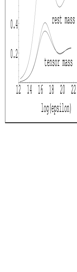
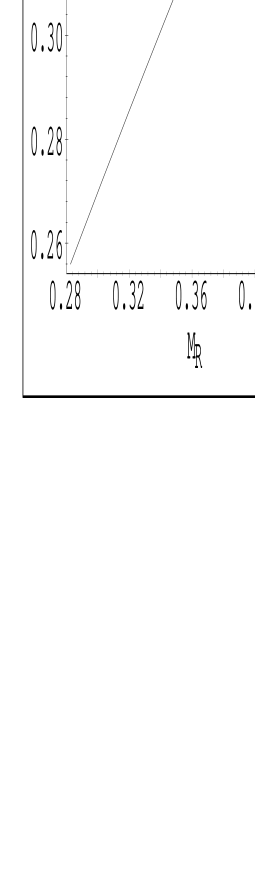
Figure 1: a) $M-log(\varepsilon_{c})$ dependence.                 b) $M_{T}-M_{R}$ dependence.      

First we concentrate our attention on the case of non-interacting neutron gas. In Fig. 1a) the dependence of the three masses $M_{T}$,$M_{K}$,$M_{R}$ on the central density $\varepsilon_{c}$ is shown. The appearance of a cusp in Fig. 1b) , where the dependence of the tensor mass $M_{T}$ on the rest mass $M_{R}$ is presented, shows that their maxima lie at the same point. Although, the maxima of the rest mass $M_{R}$ and Keplerian mass $M_{K}$ are too close in Fig. 1a) they don’t lie at the same point, as it may be seen from Fig. 2a) which shows the dependence of $M_{K}$ on $M_{R}$. We see also that Keplerian mass is considerably greater than the tensor one – about three times.

In Fig. 3a) the $M_{T}-R$ dependence is represented. It’s seen that the $M_{T}-R$ curve in our case is fairly similar to the one of general relativity, but there are significant differences, too. The maximum mass ${M_{T}}_{max}$ in our case is $\approx 0.35M_{\bigodot}$, while in general relativity the Oppenheimer-Volkoff’s mass is $M_{OV}=0.7M_{\bigodot}$. The radius corresponding to the mass $M_{\bigodot}$ is $R=4.2km$, while in the case of general relativity $R=9.6km$. If we look at Fig. 2b) where the dependence of $M_{T}$ on the central density ${\varepsilon}_{c}$ is shown, we note that ${M_{T}}_{max}$ lies at ${\varepsilon}_{c}\approx 4.5*10^{16}g/{cm}^{3}$, while $M_{OV}$ lies at ${\varepsilon}_{c}\approx 5*10^{15}g/{cm}^{3}$ in general relativity. The average density in our case is about $4$ times greater than the one in general relativity. Hence, in the model under consideration the neutron star is more compact and has a mass about $1/2$ - times smaller than $M_{OV}$. In Fig. 3b) the dependence of Keplerian mass on the star radius is presented. It’s seen that the Keplerian mass is about $1.5$ times greater than $M_{OV}$.

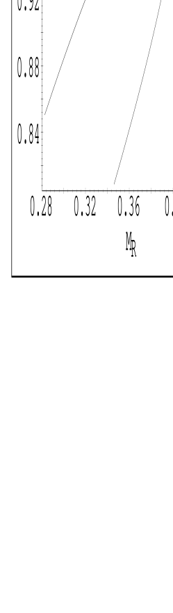
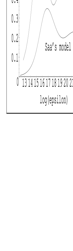
Figure 2: a) $M_{Kepler}-M_{R}$ dependence.                  b) $M_{T}-log(\varepsilon_{c})$ dependence.     

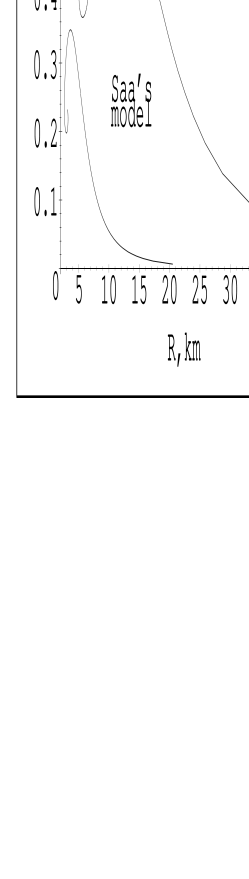
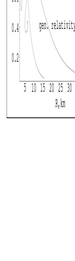
Figure 3: a) $M_{T}-R$ dependence.                      b) $M_{Kepler}-R$ dependence.          

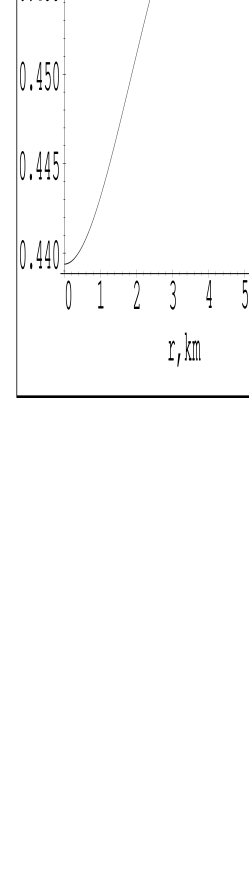
Figure 4: a) $k-r$ dependence.                  b) $K-log(\varepsilon_{c})$ dependence.     

In the Fig. 4a) the dependence $k(r)$ is shown inside the star (for central density $7.5*10^{15}g/{cm}^{3}$). In accordance to the general considerations $k$ increases from the center of the star to the surface, where $k$ takes a value $K=k(R)\approx 0.45-0.46$, which is close to $0.5$. The dependence $K(\varepsilon_{c})$ of $K$ on the star central density $\varepsilon_{c}$ is shown in Fig. 4b). It’s seen that $K$ decreases when density increases, which is similar to the previous case. So, the ratio of the torsion force to the gravitational one takes its minimum value at the center of the star and is the greatest at the surface.

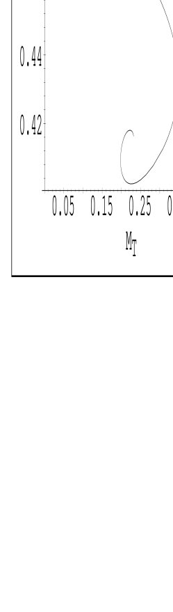
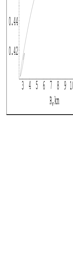
Figure 5: a) $K-M_{T}$ dependence.                      b) $K-R$ dependence.          

As it may be seen from Fig. 5a) expressing the dependence $K(M_{T})$, the torsion-urged effects are relatively strongest in the case of small masses – with increasing of the star mass (up to the point where the star loses its stability) $K$ decreases. It’s seen from Fig. 5b), where the dependence of $K$ on the star radius $R$ is shown, that in the area of stability $K$ decreases when $R$ decreases too – the more compact stars are, the smaller $K$ they have.

Fig. 6a) presents the dependencies $\theta(r)$ and $\nu(r)$ inside the star. One may see that ${1\over 2}\nu-3\Theta<0$ everywhere. The dependencies $m_{T}(r)$,$m_{Kepler}(r)$ and $m_{\theta}(r)$ are shown in Fig. 6b) for central density $7.5*10^{15}$. As it has already mentioned all masses increase with $r$.

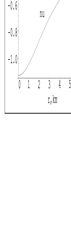
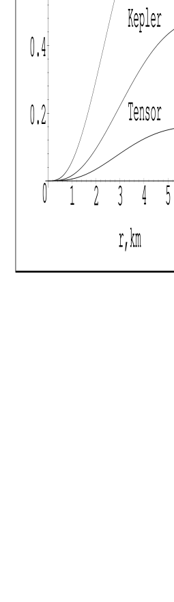
Figure 6: a) $\Theta,\nu-r$ dependence.                  b)$m_{T},m_{Kepler},m_{\theta}-r$ dependence.      

The following figures illustrate the case of Tsuruta-Cameron equation of state (TCES).

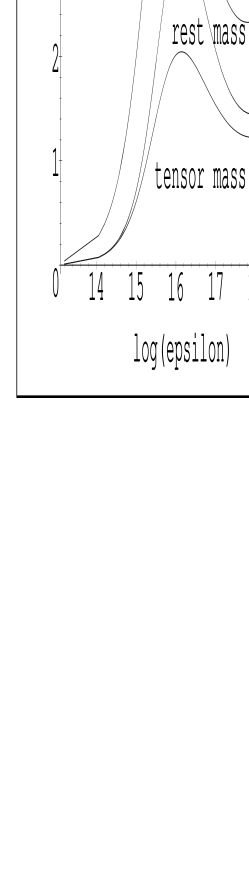
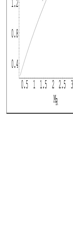
Figure 7: TCES. a) $M-log(\varepsilon_{c})$ dependence .            b) $M_{T}-M_{R}$ dependence.           

We see from the figures that the maximum tensor mass in this case is about $2M_{\bigodot}$ and the corresponding radius is about $7.5km$ - the same quantities in general relativity are correspondingly $\approx 1.6M_{\bigodot}$ and $\approx 11.5km$. Hence, the interaction between the nucleons leads to an increase in the maximum mass, as in general relativity.

Note the differences between the Fig. 5b) and Fig. 6b) (for the case of non-interacting neutron gas), and the corresponding Fig. 11b) and Fig. 12b) (for the case of Tsuruta-Cameron equation of state). There one can see the strong dependence of some results in the Saa’s model of gravity with propagating torsion on the equation of state of star’s matter.

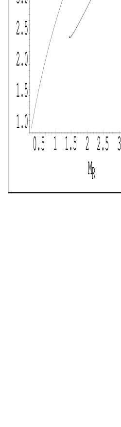
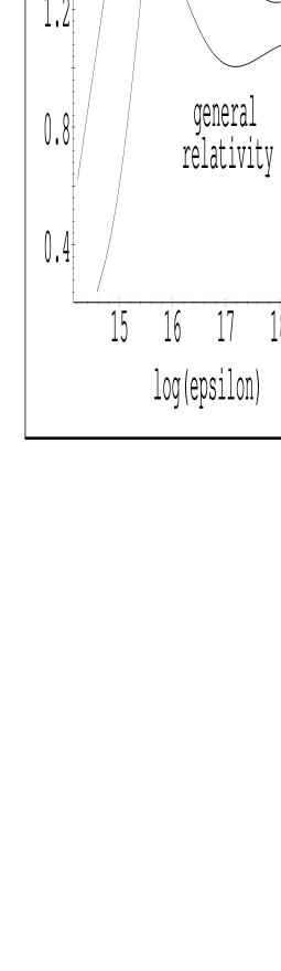
Figure 8: TCES. a)$M_{Kepler}-M_{R}$ dependence.     b) $M_{T}-log(\varepsilon_{c})$ dependence.         

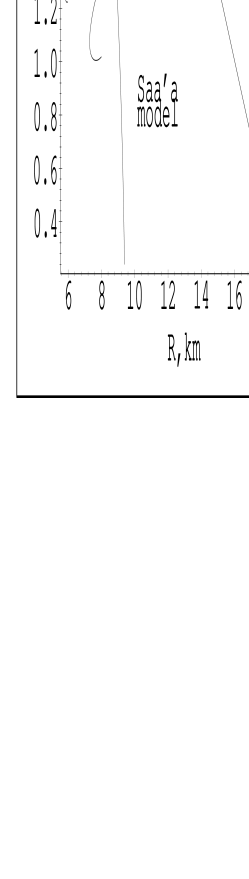
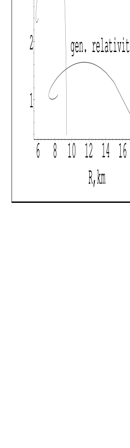
Figure 9: TCES. a) $M_{T}-R$ dependence.               b) $M_{Kepler}-R$ dependence.               

Figure 10: TCES. a) $k-r$ dependence.             b) $K-log(\varepsilon_{c})$ dependence.                          

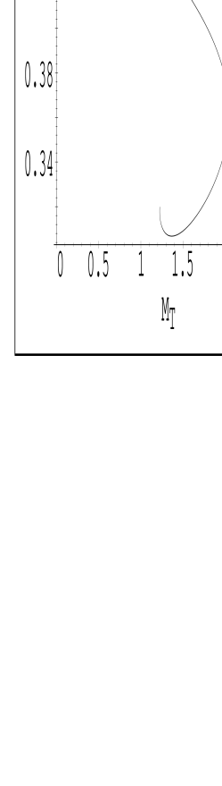
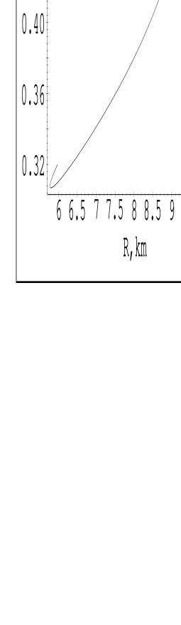
Figure 11: TCES. a) $K-M_{T}$ dependence.             b) $K-R$ dependence.                          

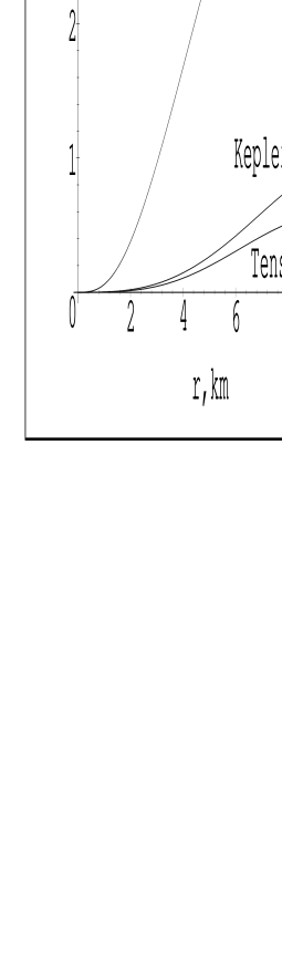
Figure 12: TCES. a) $\Theta,\nu-r$ dependence.             b) $m_{T},m_{Kepler},m_{\theta}-r$ dependence.                          

We have also examined the Harrison-Wheeler’s equation of state [25]. As in general relativity the numerical results are very close to these for the noninteracting neutron gas. For example the maximum tensor and Keplerian mass is correspondingly $\approx 0.35M_{\bigodot}$ and $\approx 1M_{\bigodot}$, and the corresponding radius is $3.8km$.

Other equations of state (of politropic type) have been examined, too. The corresponding maximum tensor mass of a neutron star reaches a value about $2.5-2.6M_{\bigodot}$, while the corresponding Keplerian mass is about $6-6.5M_{\bigodot}$.

As it is seen from numerical calculations the tensor mass and Keplerian mass differ very significantly from each other. This behaviour of the masses is qualitatively the same as in the case of a boson star in Brans-Dicke theory with $\omega=-1$ [24]. Saa’s model corresponds to the value of the Brans-Dicke parameter $\omega=-{4\over 3}$ which is close to $-1$. That’s why the observed qualitative agreement is natural. Hence, including a scalar field with an approximately the same $\omega$ in physically different kinds of stars we find similar departures of the corresponding predictions of general relativity.

This conclusion holds also in the case of large $\omega$. For example, in [5] and [7] Brans-Dicke boson star has been considered with $\omega=400$. There the results are quite similar to corresponding ones in general relativity which is just the limit $\omega\to\infty$. The star is a bit lighter but has a higher density in future.

6 Stability analysis via catastrophe theory

Methods of catastrophe theory have recently been applied for investigation the stability of self-gravitating systems as neutron and boson stars in [26] and [27] (in the case of boson stars see also [6] and [7]).

Here we discuss briefly the important question of the stability of a neutron star in our case using tools of catastrophe theory.

The basis for the stability analysis are figures Fig.1b and Fig.7b. The conserved quantities which we use to calculate the binding energy are the tensor mass and the rest mass (particle number). Drawing them against each other we obtain so-called bifurcation diagram. Actually, Fig.1b and Fig.7b are bifurcation diagrams. When the central density increases one meets a cusp. The appearance of a cusp itself isn’t enough to conclude that the stability of the neutron star changes. However, if it’s known that the star is stable along the first brunch then it will become unstable along the second brunch. In general relativity the stability of the neutron stars for small central densities is proved by using linear perturbation analysis. As it’s seen from the figures, the behaviour of the basic conserved quantities in our case is qualitatively the same as in general relativity. That’s why it’s natural to assume that for small central densities, i.e. along the first brunch the star in our case is stable against small radial perturbations. Besides of that the first brunch is composed completely of negative binding energy states which shows that it is potentially stable.

Making use of the above considerations we can conclude that the neutron stars with central densities from small values to the cusp are stable. Beyond the cusp one radial perturbation mode develops instability and the star becomes unstable.

7 Saa’s model, Roll-Krotkov-Dicke, Braginsky-Panov and Eötvosh experiments

Despite the obvious beauty of Saa’s model we shall show that it contradicts to the experiments by Roll-Krotkov-Dicke, Braginsky-Panov and Eötvosh. To do this we need the equation of motion of an isolated test body corresponding to the model under consideration. In our case the local conservation law for energy-momentum tensor can be written in the form (see (14) and (11))

$${\stackrel{{\scriptstyle\{\}}}{{\nabla}}}{}_{\sigma}(e^{-3\Theta}T_{\alpha}^{\sigma})=3e^{-3\Theta}\left({\cal L}_{M}-{{\,\,\hbox{${\frac{1}{3}}$}}}{\delta{\cal L}_{M}\over\delta\Theta}\right)S_{\alpha}.$$ (59)

Defining the four-momentum and the mass-center of a small test body as

$$P^{\alpha}=\int T^{\alpha 0}\sqrt{|g|}e^{-3\Theta}d^{3}x,$$

$$X^{\beta}={\int x^{\beta}T^{00}\sqrt{|g|}e^{-3\Theta}d^{3}x\over P^{0}}$$

and following the same procedure as in general relativity [34], [35] we obtain the equation of motion of such body in our case:

$$P^{0}{d^{2}X^{\beta}\over d{x^{0}}^{2}}+{\stackrel{{\scriptstyle\{\}}}{{\Gamma}}}_{\mu\nu}{}^{\beta}(X)E^{\mu\nu}=\left({\stackrel{{\scriptstyle\{\}}}{{\Gamma}}}_{\mu\nu}{}^{0}(X)E^{\mu\nu}\right){dX^{\beta}\over dx^{0}}+S^{\beta}(X)\Lambda-S^{0}(X)\Lambda{dX^{\beta}\over dx^{0}}$$ (60)

where

$$E^{\mu\nu}=\int T^{\mu\nu}\sqrt{|g|}e^{-3\Theta}d^{3}x$$

and

$$\Lambda=3\int\left({\cal L}_{M}-{{\,\,\hbox{${\frac{1}{3}}$}}}{\delta{\cal L}_{M}\over\delta\Theta}\right)\sqrt{|g|}e^{-3\Theta}d^{3}x.$$

We consider a static spherically-symmetric case and therefore we put $S^{0}=0$. Fixing a local inertial frame in which the test body is at rest at the moment considered and the Christoffel symbols vanish at the location of body we have

$$M{d^{2}X^{\beta}\over dt^{2}}=S^{\beta}(X)\Lambda$$ (61)

where $M$ is the inertial mass of the small test body.

Therefore in the model under consideration test bodies with different $\Lambda$ would accelerate differently in the solar field (or in the earth’s field). In good approximation we can consider the test body as built by electromagnetically interacting particles in gravitational and torsion field, i.e. the Lagrangian density for the test body is taken in the form

$${\cal L}_{M}={\cal L}^{em}_{M}+{\cal L}^{pf}_{M}$$ (62)

where

$${\cal L}^{em}_{M}=-{1\over 16\pi}F^{\mu\nu}F_{\mu\nu},$$

$${\cal L}^{pf}_{M}=-A^{\mu}J_{\mu}-\sum_{i}{m_{i}\over\sqrt{|g|}e^{-3\Theta}}{ds_{i}\over dt}\delta(\vec{x}-\vec{x}_{i}(t)),$$

and

$$J^{\mu}=\sum_{i}{q_{i}\delta(\vec{x}-\vec{x}_{i}(t))\over\sqrt{|g|}e^{-3\Theta}}{dx^{\mu}\over dt}$$

(for Lagrangian density for particles in Saa’s model see [20]). It can be shown that

$${\cal L}^{pf}_{M}-{{\,\,\hbox{${\frac{1}{3}}$}}}{\delta{\cal L}^{pf}_{M}\over\delta\Theta}=0.$$ (63)

Consequently we obtain

$$\Lambda=3\int\left({\cal L}_{M}-{{\,\,\hbox{${\frac{1}{3}}$}}}{\delta{\cal L}_{M}\over\delta\Theta}\right)\sqrt{|g|}e^{-3\Theta}d^{3}x=3\int\left({\cal L}^{em}_{M}-{{\,\,\hbox{${\frac{1}{3}}$}}}{\delta{\cal L}^{em}_{M}\over\delta\Theta}\right)\sqrt{|g|}e^{-3\Theta}d^{3}x=$$

$$-3\int{1\over 8\pi}\left({\vec{E}}^{2}-{\vec{H}}^{2}\right)\sqrt{|g|}e^{-3\Theta}d^{3}x=-3\left({\cal E}_{e}-{\cal E}_{m}\right).$$ (64)

Here ${\cal E}_{e}$ and ${\cal E}_{m}$ are correspondingly the electric and the magnetic energy containt of the test body. Therefore from (61) we have

$${d^{2}X^{\beta}\over dt^{2}}=-3S^{\beta}(X){{\cal E}_{e}-{\cal E}_{m}\over M}.$$ (65)

For aluminum and platinum the magnetic energy is small compared to the electric one. The ratio ${{\cal E}_{e}\over M}$ for aluminum and platinum is [35]

$$\left({{\cal E}_{e}\over M}\right)_{Al}=1.7*10^{-3},$$ (66)

$$\left({{\cal E}_{e}\over M}\right)_{Pt}=4.5*10^{-3}.$$ (67)

On Earth we have

$$\left({d^{2}X_{i}\over dt^{2}}\right)_{Al}-\left({d^{2}X_{i}\over dt^{2}}\right)_{Pt}=-3\left(\left({{\cal E}_{e}\over M}\right)_{Al}-\left({{\cal E}_{e}\over M}\right)_{Pt}\right)S_{i}=8.4*10^{-3}S_{i},$$ (68)

$i$ runs from $1$ to $3$.

Out of the source the gravitational potential and the torsion vector are related by $S_{i}=KU{,i}$ (see (22)) and therefore

$$\left({d^{2}X_{i}\over dt^{2}}\right)_{Al}-\left({d^{2}X_{i}\over dt^{2}}\right)_{Pt}=8.4*10^{-3}KU_{,i}.$$ (69)

According to the experiments of Roll-Krotkov-Dicke [36] and Braginsky-Panov [37] the acceleration of aluminum and platinum don’t differ by 1 part of $10^{11}$ or $10^{12}$ of $U_{,i}$ respectively in the solar gravitational field. Taking into account that ${1\over 3}\leq K\leq{1\over 2}$ we conclude that Saa’s model contradicts to these experiments.

It’s not difficult to see that Saa’s model contradicts to the experimental data in Eötvos experiment, too. Indeed, according to Eötvos experiment the acceleration of the bodies of different materials in Earth’s gravitation field don’t differ by 1 part of $10^{11}$ of $g$ [42] (or $10^{12}$ according to [43]) . Using again relation (69) and inequality ${1\over 3}\leq K\leq{1\over 2}$ we see that Saa’s model contradicts to Eötvos experiment.

8 Summary

In this article we have examined the basic spherically symmetric stationary state of stars in the Saa’s model of gravity with propagating torsion.

In the model under investigation there is no need to consider unknown charges creating the torsion-dilaton field. Its source is the very spinless matter. The whole geometry of the space-time (including metric and torsion) is determined by the familiar properties of this matter.

The parameters of the vacuum solution are determined only by the spinless matter without adopting an existence of new properties, too. In contrast to the corresponding models in the general relativity here we have two parameters $K$ and $a$ of the vacuum solutions. The values of these parameters depend on the mass distribution in the star which is related with the equation of state of the star’s matter. For a fixed equation of state both parameters become functions only of the star mass, but these functions are not the same for the different equations of state. The first parameter $K$ being the ratio of the magnitude of torsion-dilaton force and of the magnitude of gravitational force for realistic equations of matter state takes values in the interval $[{1\over 3},{1\over 2}]$, depending on the star’s mass. The second one – $a$ is analogous to the gravitational radius in general relativity and takes positive values depending on the value of the parameter $K$ and on the value of the star’s mass.

To be specific in the present article we restrict our attention to the model of neutron stars where the effects of nonlinearity are essential as in general relativity. Numerical results and analytical considerations show that the space-time torsion may have a significant role in their structure. The new torsion force decrease in some extent the role of the gravity in the star configuration and may lead to an increasing or decreasing of the maximum neutron star mass depending on the equation of state.

The complete investigation of the consistence of the whole Saa’s model of gravity with propagating torsion (including all type of physical fields) with the reality is still an open problem. The results of the present article may have not only independent value, but are necessary for reaching the solution of this critical problem. For example, after the first version of the present article was send for publication a new results based on it which show the inconsistency of Saa’s model with solar system gravitational experiments were found and published independently [38].

Saa’s model is a simple model based on pure geometrical reasons which allows to overcome a basic difficulties of the old models of gravity with torsion: the inconsistency of the application of the minimal coupling principle in action principle and directly in the equations of motion [15]. Moreover, it leads to propagating torsion which is another important physical property of this model. Unfortunately, it is not compatible with basic physical experiments. This means that one has to modify this model preserving its important new physical properties in a proper way to comply with real physics. A new investigations in this direction are in progress (see for example [39], [40]).

Nevertheless the model under consideration contradicts to basic experiments its detailed investigation is quite instructive because Saa’s model is a special case of scalar-tensor theory of gravity with a nonminimal coupling of the scalar torsion-dilaton field with matter. A similar, but more general coupling of string-dilaton can be expected in the string theory and it leads different physical effects. For example, in the article by Damour and Polyakov [41] as a consequences of nonminimal coupling between matter and dilaton was derived a violation of the equivalence principle, as far as some string-dilaton effects in the early universe [41]. Unfortunately, the present days string theory is not able to predict definitely the form of the coupling between string-dilaton and the real matter. In contrast, Saa’s model is the only one we know with complete determined interaction of the (torsion) dilaton with all kinds of matter. This interaction is similar to the one expected in other models. In the present article it is shown at first that the nonminimal coupling of the dilaton field with the matter will emerge in extreme conditions in a neutron star and that it leads to clear new physical phenomena of different kind, some details of which may depend on the equation of matter state. Most probably similar effects will appear in other possible modifications of the theory of torsion-dilaton, as far as in the other types of theories of dilaton. For example the neutron stars may give us a way to a real physics in string theories if the string-dilaton interactions with real matter will be established. Hence, the most important conclusion of present article is that looking for physical manifestation of the dilaton one has to investigate in details its influence on the neutron star structure.

Acknowledgments

We are deeply grateful to the unknown referees who suggested to consider different types of masses of the neutron star in Saa’s model and stability analysis of the neutron star via catastrophe theory, and to add to the present paper results about the consistence of this model with physical reality, as far as for pointing out the references [2], [5], [6], [7], [9], [10], [24], [26] and [27]. The work on this article has been partially supported by the Sofia University Foundation for Scientific Researches, Contracts No.No. 245/97, 257/97, and by the Bulgarian National Foundation for Scientific Researches, Contract No. F610/97. One of us (PF) is grateful to the leadership of the Bogoliubov Laboratory of Theoretical Physics, JINR, Dubna, Russia for hospitality and working conditions during his stay there in the summer of 1998 when a part of this investigation has been completed.

References

- [1] Green M B, Schwarz J H, Witten E, 1987 Superstring theory Cambridge University Press, Cambridge
- [2] Dereli, Tucker, 1995 Class. Quant. Grav. 12 L25
- [3] Damour T, Esposito-Farese G, 1993 Phys. Rev. Lett. 70 2220
- [4] Barrow J, 1992 Phys. Rev. D46 3227
- [5] Torres D, Liddle A, Schunck F, 1998 Phys. Rev. D57 4821
- [6] Comer G, Shinkai H, 1998 Class. Quant. Grav. 15 669
- [7] Torres D, Schunk F, Liddle A, 1998 Class. Quant. Grav. 15 3701
- [8] Hojman S, Rosenbaum M, Rayn M, Shepley L, 1978 Phys. Rev. D17 3141
- [9] Hojman S, Rosenbaum M, Rayn M, 1979 Phys. Rev. D19 430
- [10] De Sabbata V, Gasperini M, 1981 Phys. Rev. D23 2116
- [11] Hehl F, Von der Heyde P, Kerlick G, 1976 Rev. Mod. Phys. 48 393
- [12] Hehl F, McCrea J, Mielke E, Ne’eman Y, 1995 Phys. Rep. 258 1
- [13] Gronwald F, Hehl F, 1996 in the Proc. of the 14th Course of the School of Cosmology and Gravitation on Quantum Gravity, Erice, Italy, May 1995, ed. P. Bargman, V. de Sabbata, and H. Treder, World Scientific, Singapore
- [14] Carrol S, Field G, 1994 Phys. Rev. D50 3867
- [15] Saa A, 1997 Gen. Rel. and Grav. 29 205
- [16] Saa A, 1993 Mod. Phys. Lett. A8 2565
- [17] Saa A, 1994 Mod. Phys. Lett. A9 971
- [18] Saa A, 1995 Class. Quant. Grav. 12 L85
- [19] Saa A, 1995 J. Geom. and Phys. 15 102
- [20] Fiziev P P, 1998 Gen. Rel. Grav. 30, 1341
- [21] Brans C, 1961 Phys. Rev. 125 2194
- [22] Xanthopoulos B C, Zannias T, 1989 Phys. Rev. D40 2564
- [23] Lee D L, 1974 Phys. Rev. D10 2374
- [24] Whinnett A W, 1997 Mass definitions for Boson Stars in Brans-Dicke Gravity, E-print: gr-qc/9711080.
- [25] Harrison B K, Thorn K S, Wakano M, Wheeler J A, 1965 Gravitation theory and Gravitational collapse, University of Chicago Press
- [26] Kusmartsev F, Mielke E, Schunk F , 1991 Phys. Rev. D43 3895
- [27] Kusmartsev F, Mielke E, Schunk F , 1991 Phys. Lett. A157 465
- [28] Shapiro S L, Teukolsky S A, 1983 Black Holes, White dwarfs and Neutron stars. The physics of Compact Objects, Wiley, N. Y.
- [29] Zel’dovich Ya B, 1961 Zh. Eksp. Teor. Fiz. 37 569
- [30] Zel’dovich Ya. B., Novikov I. D., 1971 Stars and Relativity, The University of Chicago Press
- [31] Tsuruta S, Cameron A G W, 1966 Can. J. Phys. 44 1895
- [32] Tolman R C, 1962 Relativity, Thermodynamics and Cosmology, Oxford University Press, N. Y.
- [33] Landau L D, Lifshitz E M, 1962 Statistical Mechanics, Vol. 5 of Course of Theoretical Physics, Pergamon, Oxford
- [34] Synge J L, 1960 Relativity: The general theory, Amsterdam
- [35] Ni W.-T, 1979 Phys. Rev. D19 2260
- [36] Roll P, Krotkov R, Dicke R, 1964 Ann. Phys. (N. Y.) 26 442
- [37] Braginsky V, Panov V , 1971 Zh. Eksp. Teor. Fiz. 61 873
- [38] Fiziev P, Yazadjiev S, 1998, Solar-system experiments and Saa’s model of gravity with propagating torsion, preprint JINR, Dubna E-98-219; E-print gr-qc/9806063
- [39] Fiziev P, 1998 Gravitation Theory with Propagating Torsion, E-print gr-qc/9808006
- [40] Fiziev P, 1998 Torsion Dilaton and Novel Minimal Coupling Principle, E-print gr-qc/9809001
- [41] Damour T, Polyakov A , 1994 Nucl.Phys. B423 532
- [42] Will C, 1993 Theory and Experiment in Gravitational Physics Cambridge University Press
- [43] Su Y,Heckel B,Adelberger E,Gundlach J,Harris M,Smith G, Swanson H, 1994 Phys. Rev. D50 3614