Quasi-Spherical Light Cones of the Kerr Geometry

Frans Pretorius and Werner Israel

Canadian Institute for Advanced Research Cosmology Program
Department of Physics and Astronomy
University of Victoria
P.O. Box 3055 STN CSC
Victoria B.C., Canada V8W 3P6

Quasi-spherical light cones are lightlike hypersurfaces of the Kerr geometry that are asymptotic to Minkowski light cones at infinity. We develop the equations of these surfaces and examine their properties. In particular, we show that they are free of caustics for all positive values of the Kerr radial coordinate $r$. Useful applications include the propagation of high-frequency waves, the definition of Kruskal-like coordinates for a spinning black hole and the characteristic initial-value problem.

PACS numbers: 0240, 0420

1 Introduction

The Kerr geometry is a vacuum spacetime with a Weyl tensor of Petrov type D. According to the Goldberg-Sachs theorem [1], it therefore possesses two congruences (ingoing and outgoing) of shear-free lightlike geodesics. Historically, these congruences played an essential role in the discovery of the Kerr solution [2], because the metric takes a simple explicit form in coordinates adapted to them.

In the original [2],[3] (Eddington-Kerr) form of the metric, the ingoing congruence consists of parametric curves of the Eddington- Kerr coordinate $v$, often referred to as an “advanced time”. This nomenclature can be misleading, because hypersurfaces of constant $v$ are actually spacelike, not lightlike, if the Kerr rotational parameter $a$ is nonzero. (The lightlike congruences are “twisting”, i.e., not orthogonal to any hypersurfaces, and hence not tangent to lightlike hypersurfaces if $a\neq 0$).

Thus, the Eddington-Kerr form of the metric, and the Boyer-Lindquist form [3] derived from it by an elementary coordinate transformation, correspond to a “threading” [4] (i.e., a one-dimensional foliation) of the manifold by twisting lightlike geodesics. However, a “slicing” (three dimensional foliation), in particular a light-like slicing, is for many purposes more advantageous and often corresponds more closely to the physics.

Light cones of the Kerr geometry have not previously been a subject of systematic study to our knowledge. Perhaps this stems in part from a feeling that such hypersurfaces would quickly develop caustics because of the twist inherent in the metric. Yet as characteristics these surfaces obviously play a key role in the physics of Kerr black holes, e.g in the propagation of wave fronts and high-frequency waves, and in characteristic initial value problems.

In this paper we first derive the general solution for axisymmetric lightlike hypersurfaces of the Kerr geometry (Sec. 2). We then focus on a particular foliation (invariant under time-displacement) by (either ingoing or outgoing) “quasi-spherical” light cones, defined as degenerate 3-spaces whose spatial sections are asymptotically spherical at infinity. These hypersurfaces become the standard Minkowski light cones when the Kerr mass parameter $m$ vanishes; if $a=0$, $m\neq 0$, they are the familiar spherical light cones, $t\pm{r_{\ast}}=constant$, of Schwarzschild spacetime (where ${r_{\ast}}$ is the “tortoise” coordinate). Quite generally, for arbitrary $m\geq 0$ and $a$, they have the remarkable property of being free of caustics for all positive values of the Kerr radial coordinate $r$.

These appealing features suggest that coordinates adapted to quasi- spherical surfaces should be especially convenient and useful for the description of the Kerr geometry. The drawback (and it is considerable) is that the metric is no longer expressible in an explicit elementary form, because the new coordinates are elliptic functions of the Boyer-Lindquist coordinates.

We now briefly outline the contents of the paper. We begin in Sec. 2 by solving the eikonal equation for axisymmetric lightlike hypersufaces of the Kerr geometry. The general solution is expressed in terms of integrals of elliptic type, and involves an arbitrary function $f$ of one variable, to be fixed when the “initial” (e.g. asymptotic) shape of the surface is given. (If $m=0$ the geometry becomes flat and the integrals can be reduced to elementary form; in Sec. 3 we digress briefly to illustrate this.) Some general properties of axisymmetric lightlike surfaces are developed in Sec. 4. In Sec. 5, guided by the results of Sec. 3 for Minkowski light cones, we make the special choice of $f$ appropriate for asymptotically spherical light cones in Kerr space. The key result, that these are free of caustics for $r>0$, is demonstrated in Sec. 6. In Secs. 7 and 8 we show how the “quasi-spherical” coordinates ${r_{\ast}}$, ${\theta_{\ast}}$ defined by these light cones can be used to construct high-frequency solutions to the wave equation and Kruskal-like coordinates for Kerr black holes. Sec. 9 summarizes the limiting cases that can provide serviceable approximations for the elliptic functions which appear in the quasi-spherical form of the metric. Finally, in Sec. 10 we present some results of numerical integrations for the inward evolution of the light cone generators.

2 Axisymmetric lightlike hypersurfaces

The equation of an arbitrary axially symmetric lightlike hypersurface of the Kerr geometry is expressible in terms of elliptic integrals as we now proceed to show.

We write the Kerr metric in its standard (Boyer-Lindquist) form

$$ds^{2}=\frac{\Sigma}{\Delta}dr^{2}+\Sigma d\theta^{2}+R^{2}\sin^{2}\theta d\phi^{2}-\frac{4mar\sin^{2}\theta}{\Sigma}d\phi dt-\left(1-\frac{2mr}{\Sigma}\right)dt^{2},$$ (1)

where

$$\Sigma=r^{2}+a^{2}\cos^{2}\theta,\ \ R^{2}=r^{2}+a^{2}+\frac{2ma^{2}r\sin^{2}\theta}{\Sigma},\ \ \Delta=r^{2}+a^{2}-2mr,$$ (2)

and we note the useful identities

$$\Sigma R^{2}=(r^{2}+a^{2})^{2}-\Delta a^{2}\sin^{2}\theta,$$ (3)

$$g_{\phi\phi}g_{tt}-g_{\phi t}^{2}=-\Delta\sin^{2}\theta.$$ (4)

The equation

$$v(t,r,\theta)=t+\epsilon{r_{\ast}}(r,\theta)=constant,\ \ \epsilon=\pm 1$$ (5)

represents an axisymmetric lightlike hypersurface (ingoing for $\epsilon=1$, outgoing for $\epsilon=-1$) if $g^{\alpha\beta}(\partial_{\alpha}v)(\partial_{\beta}v)=0$, i.e., if

$$\Delta(\partial_{r}{r_{\ast}})^{2}+(\partial_{\theta}{r_{\ast}})^{2}=(r^{2}+a^{2})^{2}/\Delta-a^{2}\sin^{2}\theta.$$ (6)

It is easy to obtain a particular (separable) solution of (6) depending on two arbitrary constants (a “complete integral”) by adding and subtracting an arbitrary separation constant $a^{2}\lambda$ on the right -hand side. Let us define

$$P^{2}(\theta,\lambda)=a^{2}(\lambda-\sin^{2}\theta),\ \ \ Q^{2}(r,\lambda,m)=(r^{2}+a^{2})^{2}-a^{2}\lambda\Delta.$$ (7)

(Note the useful identity

$$Q^{2}+\Delta P^{2}=\Sigma R^{2},$$ (8)

which follows from (3).) A complete integral

$${r_{\ast}}=\rho(r,\theta,\lambda,m),$$ (9)

of (6) is then obtained by integrating the exact differential

$$d{r_{\ast}}=(Q/\Delta)dr+Pd\theta$$ (10)

at fixed $\lambda$. When (10) is integrated, a second, additive integration constant appears which we shall denote as $a^{2}f(\lambda)/2$, where $f$ is an arbitrary function.

We next proceed in the usual way to promote this complete integral, depending upon the arbitrary constants $\lambda$ and $f(\lambda)$, to a general solution involving an arbitrary function.

In (9), $\rho$ is a function of three independent variables $r$, $\theta$ and $\lambda$ (not counting $m$ and $a$), and a more complete expression for its differential is

$$d\rho=(Q/\Delta)dr+Pd\theta+(a^{2}/2)Fd\lambda,$$ (11)

where $F$ is the partial derivative

$$(a^{2}/2)F(r,\theta,\lambda,m)=\partial_{\lambda}\rho(r,\theta,\lambda,m).$$ (12)

Its explicit form may be taken to be

$$F(r,\theta,\lambda,m)=\int_{0}^{\theta}\frac{d\theta^{\prime}}{P(\theta^{\prime},\lambda)}+\int_{r}^{\infty}\frac{dr^{\prime}}{Q(r^{\prime},\lambda)}+f^{\prime}(\lambda).$$ (13)

Up to now, we have taken $\lambda$ to be a constant, i.e., $d\lambda=0$ in (11). But we achieve the same effect (i.e., (11) still reduces to (10) ) even when $d\lambda\neq 0$ provided we require that $F=0$. In other words: the function ${r_{\ast}}(r,\theta)$, given by (9) with $\lambda$ now a function $\lambda(r,\theta)$, remains a solution of (6) provided its extra dependence on $r,\theta$ through $\lambda$ does not change the algebraic form of the differential (10). This will indeed be so if we impose the constraint

$$F(r,\theta,\lambda,m)=0.$$ (14)

This condition fixes the dependence of $\lambda$ on $r,\theta$ for any given choice of $f(\lambda)$. Thus we now have a general solution, depending upon an arbitrary function $f[\lambda(r,\theta)]$.

The explicit form of the general solution (9) is then

$$\rho(r,\theta,\lambda)=\int\frac{r^{2}+a^{2}}{\Delta(r,m)}dr+\int_{r}^{\infty}\frac{r^{\prime 2}+a^{2}-Q(r^{\prime},\lambda,m)}{\Delta(r^{\prime},m)}dr^{\prime}$$ (15)

$$+\int_{0}^{\theta}d\theta^{\prime}P(\theta^{\prime},\lambda)+\frac{1}{2}a^{2}f(\lambda),$$

where the radial dependence has been arranged to ensure convergence of the definite integral at its upper limit. When performing the integrations in (13) and (15), we are allowed to treat $\lambda$ as merely a passive constant parameter – it is in fact a function of the limits of integration $r$,$\theta$, not of the integration variables – with the constraint (14) imposed a posteriori. It is possible, though not especially illuminating or useful, to express each of these integrals in terms of standard elliptic integrals.

3 The case $m=0$: light cones in Minkowski space

As a simple illustrative example (and because we shall need some of the results later), we specialize in this section to the case $m=0$. The Kerr line-element reduces to the metric of flat spacetime expressed in terms of oblate spheroidal coordinates $r,\theta$ – related to Cartesians by

$$x^{2}+y^{2}=(r^{2}+a^{2})\sin^{2}\theta,\ \ \ z=r\cos\theta.$$ (16)

The second integral in (13) can be reduced to the same general form as the first integral when $m=0$. Assume that we are in a domain where $\lambda(r,\theta)<1$. Setting

$$Q_{0}(r^{\prime},\lambda)=Q(r^{\prime},\lambda,m=0)=\sqrt{r^{\prime 2}+a^{2}}\sqrt{r^{\prime 2}+a^{2}(1-\lambda)},$$ (17)

and making the substution

$$r^{\prime}=a\sqrt{1-\lambda}\sin\chi^{\prime}/\sqrt{\lambda-\sin^{2}\chi^{\prime}},$$ (18)

we find

$$dr^{\prime}/Q_{0}=d\chi^{\prime}/a\sqrt{\lambda-\sin^{2}\chi^{\prime}}.$$ (19)

Thus the two integrals in (13) can be combined into a single integral, to give

$$aF(r,\theta,\lambda,m=0)=\int_{\chi(r,\lambda)}^{\theta}\frac{d\chi^{\prime}}{\sqrt{\lambda-\sin^{2}\chi^{\prime}}}+g^{\prime}(\lambda),$$ (20)

where

$$g(\lambda)=af(\lambda)+2\int_{0}^{{\theta_{\ast}}}\sqrt{\lambda-\sin^{2}\chi^{\prime}}d\chi^{\prime},$$ (21)

and the form of $\chi(r,\lambda)$ is given by the “unprimed” version of (18); equivalently,

$$\tan{\theta_{\ast}}=\frac{\sqrt{r^{2}+a^{2}}}{r}\tan\chi,\ \ \ \lambda\equiv sin^{2}{\theta_{\ast}}.$$ (22)

The function $g(\lambda)$ is arbitrary. As an example, let us consider the simplest choice, $g(\lambda)=0$. The functional dependence $\lambda(r,\theta)$ corresponding to this choice is determined by the constraint $F=0$, which requires that $\chi(r,\lambda)=\theta$ by inspection of (20). Thus (22) gives

$$\tan{\theta_{\ast}}=\frac{\sqrt{r^{2}+a^{2}}}{r}\tan\theta=\frac{\sqrt{x^{2}+y^{2}}}{z}$$ (23)

by (16), showing that ${\theta_{\ast}}$ is the spherical polar angle. With $\lambda(r,\theta)$ known from (23), it is straightforward to integrate (10) to obtain

$${r_{\ast}}=\sqrt{r^{2}+a^{2}\sin^{2}\theta}.$$ (24)

Thus ${r_{\ast}}$ is the usual spherical radius, and our solutions $v=t\pm{r_{\ast}}=constant$ of (6) are in this case the Minkowski light cones.

4 Axisymmetric lightlike hypersurfaces: general properties

Returning to the general case, we shall now derive a number of results applicable to all axisymmetric lightlike hypersurfaces of Kerr.

Since the function $\lambda(r,\theta)$ is determined by the constraint $F=0$, the partial derivatives of $\lambda$ can be read off from $dF=0$ (13):

$$\mu d\lambda=-dr/Q+d\theta/P,\ \ \ \mu\equiv-\partial F/\partial\lambda.$$ (25)

It follows from (10) and (25) that $\nabla{r_{\ast}}\cdot\nabla\lambda=0$, i.e. that ${r_{\ast}}$ and $\lambda$ are orthogonal with respect to the intrinsic 2-metric

$$d\sigma^{2}=\Sigma(dr^{2}/\Delta+d\theta^{2})$$ (26)

of the spatial sections $(\phi,t)=constant$ of the Kerr geometry. Since $\lambda$ is independent of $\phi$ and $t$, it follows further that $\lambda$ is constant along the lightlike generators, i.e.,

$$\ell^{\alpha}\partial_{\alpha}\lambda=0,\ \ \ \ell_{\alpha}=-\partial_{\alpha}v=-\partial_{\alpha}(t+\epsilon{r_{\ast}}).$$ (27)

If ${r_{\ast}}$ and $\lambda$ are adopted as coordinates in place of $r$ and $\theta$, the 2-metric (26) becomes

$$d\sigma^{2}=R^{-2}(\Delta d{r_{\ast}}^{2}+L^{2}d\lambda^{2}),\ \ \ L\equiv\mu PQ,$$ (28)

where we have made use of (10), (25) and (8). The identity (4) can be re-arranged in the form

$$\left(1-\frac{2mr}{\Sigma}\right)+\omega_{B}^{2}R^{2}\sin^{2}\theta=\frac{\Delta}{R^{2}},$$ (29)

where

$$\omega_{B}=-\frac{g_{\phi t}}{g_{\phi\phi}}=\frac{2mar}{\Sigma R^{2}}$$ (30)

is the Bardeen or ZAMO angular velocity $d\phi/dt$ which characterizes orbits having zero angular momentum. This enables us to recast the Kerr metric (1) in the form

$$ds^{2}=\frac{\Delta}{R^{2}}(d{r_{\ast}}^{2}-dt^{2})+\frac{L^{2}}{R^{2}}d\lambda^{2}+R^{2}\sin^{2}\theta(d\phi-\omega_{B}dt)^{2}.$$ (31)

Thus

$$g^{{r_{\ast}}{r_{\ast}}}=R^{2}/\Delta=-g^{tt},$$ (32)

from which the null character of the 3-spaces $t\pm{r_{\ast}}=constant$ is directly evident. The degenerate intrinsic metric of these 3-spaces is

$$(ds^{2})_{LL}=(L/R)^{2}d\lambda^{2}+R^{2}\sin^{2}\theta(d\phi-\omega_{B}dt)^{2},$$ (33)

showing that the generators rotate with $ZAMO$ angular velocity relative to stationary observers at infinity. (This is directly obvious from (27), which shows that $\ell_{\phi}=0$ for an axisymmetric hypersurface). From (33) we see that caustics will develop when the degenerate volume element tends to zero, i.e. when $L\sin\theta\rightarrow 0$ (recalling that $\lambda$ has a fixed value along each generator).

The integrability of (25) for the exact differential $d\lambda$ provides a condition on the integrating factor $\mu$. This takes the form of an evolution equation for $\mu$ along the generators. A straightforward calculation, which calls upon (7), (8), (13) and (25) itself, yields

$$(\partial\mu/\partial r)_{\lambda}=\frac{a^{2}}{2}\frac{\Sigma R^{2}}{P^{2}Q^{3}},$$ (34)

where the subscript $\lambda$ indicates that the partial derivative is being taken at fixed $\lambda$.

Inversion of the differential relations (10) and (25) gives

$$\Sigma R^{2}dr=\Delta Q(d{r_{\ast}}-\mu P^{2}d\lambda),\ \ \ \Sigma R^{2}d\theta=P(\Delta d{r_{\ast}}+\mu Q^{2}d\lambda),$$ (35)

which will be of use in subsequent sections.

5 Quasi-spherical light cones

From here on we confine attention to a special class, “quasi-spherical light cones”, defined as lightlike hypersurfaces which asymptotically approach Minkowski spherical light cones at infinity. Define an angle ${\theta_{\ast}}(r,\theta)$ by

$$\lambda=\sin^{2}{\theta_{\ast}}.$$ (36)

In Minkowski space, the generators $\lambda=constant$ of light cones are radial straight lines, suggesting (as we confirmed in Sec. 3) that ${\theta_{\ast}}$ is the spherical polar angle. For $r>>a$, the oblate coordinates $(r,\theta)$ become indistinguishable from spherical coordinates, so we have the condition

$${\theta_{\ast}}(r=\infty,\theta)=\theta$$ (37)

for spherical light cones in Minkowski space. This asymptotic condition must therefore also hold for quasi-spherical surfaces in Kerr space. This fixes the arbitrary function $f^{\prime}(\lambda)$ in (13). We conclude that

$$F(r,\theta,\lambda,m)=\int_{r}^{\infty}\frac{dr^{\prime}}{Q(r^{\prime},\lambda,m)}-\int_{\theta}^{\theta_{\ast}}\frac{d\theta^{\prime}}{P(\theta^{\prime},\lambda)}$$ (38)

generates the solution for quasi-spherical surfaces. The radial function $\rho(r,\theta,\lambda,m)$ is given by (15) with (compare (21) with $g(\lambda)=0$)

$$af(\lambda)=-2\int_{0}^{{\theta_{\ast}}}\sqrt{\lambda-\sin^{2}\theta^{\prime}}d\theta^{\prime}.$$ (39)

The equation of the hypersurface is then $v=t\pm{r_{\ast}}(r,\theta)=constant$, with ${r_{\ast}}=\rho(r,\theta,\lambda(r,\theta))$ and the function $\lambda(r,\theta)\equiv\sin^{2}{\theta_{\ast}}$ determined by the constraint $F=0$.

6 No caustics for positive $r$

We now prove the rather remarkable result that quasi-spherical light cones are free of caustics for all positive values of the Kerr radial coordinate $r$.

This is trivially true if $m=0$, when these surfaces are simply light cones in Minkowski space with vertices at the spatial origin, represented by $r=0$, $\theta=0$ or $\pi$ in oblate spheroidal coordinates according to (16). We shall prove that it is true a fortiori for $m>0$ by effectively showing that when $m$ is larger, the generators converge less rapidly as $r\rightarrow 0^{+}$.

As noted in Sec. 4, formation of a caustic along a generator is signalled by

$$\mu PQ\sin\theta\rightarrow 0.$$ (40)

We consider in turn the behaviour of each factor in (40) along an ingoing generator, so that $r$ is positive and decreasing, with $\lambda$ fixed. Because of the equatorial symmetry we need only consider “northern” generators, i.e., we may assume ${\theta_{\ast}}$ (which specifies the initial, asymptotic value of $\theta$ when $r=+\infty$) to be acute, and $P(\theta,\lambda)$ positive, at least initially. (Note from (10) that equatorial symmetry of ${r_{\ast}}(r,\theta)$ implies $P(\lambda,\pi-\theta)=-P(\lambda,\theta)$.)

Since $\theta$ decreases with $r$ at fixed $\lambda$ according to (25), the factor $P=a\sqrt{\lambda-\sin^{2}\theta}$ must increase and remain positive. Any possible caustic in the Kerr positive-$r$ sheet cannot arise from the behaviour of $P$.

We proceed to consider the other factors in (40). From the definition (7),

$$Q(r,\lambda,m)>Q(r,\lambda,m=0)>0\ \ \ (r>0,m>0).$$ (41)

We shall further show that

$$(\partial\theta/\partial m)_{r,\lambda}>0\ \ \ \mbox{and}\ \ \ (\partial\mu/\partial m)_{r,\lambda}>0\ \ \ (r>0,{\theta_{\ast}}<\pi/2).$$ (42)

Thus, none of the three factors $\mu$, $Q$ and $\sin\theta$ can reach zero sooner for positive $m$ than they do in flat space, and hence they do not reach zero for any positive value of $r$.

To establish (42), we note that the function $\theta(r,\lambda,m)$ is determined by the vanishing of $F(r,\theta,\lambda,m)$ as given by (38). Taking the differential at fixed $r$,$\lambda$ and using (7) gives

$$(\partial\theta/\partial m)_{r,\lambda}=a^{2}\lambda PI,\ \ \ I(r,\lambda,m)\equiv\int_{r}^{\infty}r^{\prime}dr^{\prime}/Q^{3}(r^{\prime},\lambda,m),$$ (43)

which is manifestly positive. Turning to $\mu$, this is defined as a function of $r,\theta,\lambda,m$ by $\mu=-\partial F/\partial\lambda$ according to (25). Inverting the order of partial differentiation and using (38),

$$\frac{\partial\mu}{\partial m}=-\frac{\partial}{\partial\lambda}\frac{\partial F}{\partial m}=\frac{\partial}{\partial\lambda}(a^{2}\lambda I),$$ (44)

$$\frac{\partial\mu}{\partial\theta}=-\frac{\partial}{\partial\lambda}\frac{\partial F}{\partial\theta}=-\frac{\partial}{\partial\lambda}\frac{1}{P}=\frac{a^{2}}{2P^{3}}.$$ (45)

Hence

$$\left(\frac{\partial\mu}{\partial m}\right)_{r,\lambda}=\frac{\partial\mu}{\partial m}+\frac{\partial\mu}{\partial\theta}\left(\frac{\partial\theta}{\partial m}\right)_{r,\lambda}=a^{2}\left(1+\frac{1}{2}\frac{a^{2}\lambda}{P^{2}}\right)I+\frac{3}{2}a^{4}\lambda J,$$ (46)

where

$$J(r,\lambda,m)=\int_{r}^{\infty}r^{\prime}\Delta(r^{\prime})dr^{\prime}/Q^{5}(r^{\prime},\lambda,m).$$ (47)

Each term in (46) is manifestly positive. This completes the proof.

The fact that adding mass to the Kerr field should reduce the focusing of ingoing radial light rays is at first sight paradoxical, but can be explained by the circumstance that the material source is not at the origin, but located on the singular equatorial ring $x^{2}+y^{2}=a^{2}$, $z=0$ (see (16)). The source has a peculiar, “demi-pole” structure [5], made possible by the double-sheeted structure of the Kerr manifold: a ring of positive mass in the sheet $r>0$ is bonded to a ring of negative mass in the sheet $r<0$. Light rays heading inwards toward the origin in the sheet $r>0$ are deflected outward by the ring and defocused. Repulsive effects have become dominant by the time they pass through the disk $r=0:$ the rays are then refocused and form a caustic in the sheet $r<0$. This description is more than just hand-waving: the Keres Newtonian analogue model of the Kerr field [6] has a source structure and equations of motion closely resembling Kerr (apart from frame dragging), and displays precisely this behaviour.

Figure 1 (a result of numerical integrations described in Sec. 10) shows the ingoing generators mapped onto the flat background of the Kerr-Schild decomposition, using the rectangular coordinates defined in (16). (Effects of frame dragging are not shown). According to the Keres-Kerr model, the gravitational “force” should become repulsive for $r\approx a$, and, indeed, the generators have inflection points near this radius.

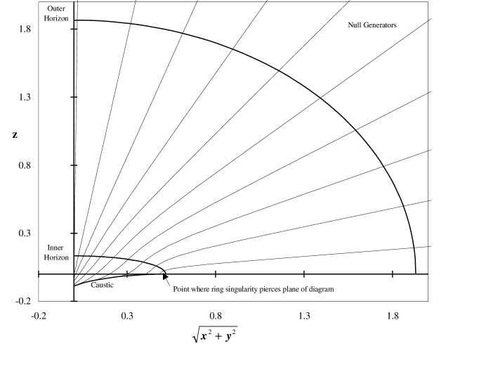
Figure 1: Null generators of the quasi-spherical light cones projected onto the Cartesian plane for $m=1$, $a=1/2$. The azimuthal twist (not shown in this two-dimensional representation) depends on the choice of azimuthal coordinate; it is zero for the coordinate $\phi_{\epsilon}$ introduced in Sec. 8. In order to follow the generators through the equatorial disk $r=0$ and into the negative-$r$ sheet, the “southern half” ($\theta>\pi/2$) of the positive-$r$ sheet has been cut away, and replaced by the “northern” half ($\theta<\pi/2$) of the negative-$r$ sheet. Note that only well within the outer horizon does the mass of the spacetime significantly affect the $r,\theta$ behaviour of the generators (which would continue as straight lines intersecting the origin if $m$ were zero). The caustic emanates from the singularity $r=0$, $\theta=\pi/2$ (if $m>0$) and creeps inwards toward the axis and “downwards” toward increasingly negative values of $r$.

7 Eikonal solution of the wave equation

Since the quasi-spherical light cones $t\pm{r_{\ast}}=constant$ are characteristics of the wave operator, the coordinates ${r_{\ast}},\lambda$ are well adapted for representing asymptotically spherical high-frequency modes.

The wave equation for $\Psi({r_{\ast}},\lambda,\phi,t)$ on the Kerr background (31) is

$$\frac{\Delta}{R^{2}}\Box\Psi=(\partial^{2}_{r_{\ast}}-\partial^{2}_{t})\Psi+(\partial_{r_{\ast}}\ln\gamma)(\partial_{r_{\ast}}\Psi)+\gamma^{-1}\partial_{\lambda}(\gamma^{-1}\Delta\sin^{2}\theta\partial_{\lambda}\Psi)+$$ (48)

$$+\left(1-\frac{2mr}{\Sigma}\right)\frac{1}{R^{2}\sin^{2}\theta}\partial^{2}_{\phi}\Psi-2\omega_{B}\partial_{\phi}\partial_{t}\Psi=0$$

where $\gamma=\mu PQ\sin\theta$ gives the area element (degenerate volume element) on the light cone (33).

Introducing the ansatz

$$\Psi=\Phi({r_{\ast}},\lambda)e^{i\omega(t+\epsilon{r_{\ast}})}e^{in\phi}\ \ \ (\epsilon=\pm 1)$$ (49)

into (48), we find

$$2\epsilon i\omega\left[\partial_{r_{\ast}}\Phi+\Phi\left(\frac{1}{2}\partial_{r_{\ast}}\ln\gamma-\epsilon in\omega_{B}\right)\right]+B=0,$$ (50)

where

$$B=\partial^{2}_{r_{\ast}}\Phi+(\partial_{r_{\ast}}\ln\gamma)(\partial_{r_{\ast}}\Phi)+\gamma^{-1}\partial_{\lambda}(\gamma^{-1}\Delta\sin^{2}\theta\partial_{\lambda}\Phi)-\frac{n^{2}}{R^{2}\sin^{2}\theta}\left(1-\frac{2mr}{\Sigma}\right)\Phi$$ (51)

has no explicit $\omega$-dependence. We can re-express $\omega_{B}$ in (50) as a partial derivative with respect to ${r_{\ast}}$. Defining an angular function

$$\alpha(r,\lambda)=\int^{r}\frac{2mar^{\prime}}{\Delta(r^{\prime})Q(r^{\prime},\lambda)}dr^{\prime}$$ (52)

and recalling (35),we find

$$\left(\frac{\partial\alpha}{\partial{r_{\ast}}}\right)_{\lambda}=\frac{2mar}{\Delta Q}\left(\frac{\partial r}{\partial{r_{\ast}}}\right)_{\lambda}=\frac{2mar}{\Sigma R^{2}}=\omega_{B}.$$ (53)

Therefore (50) can be rewritten

$$2\epsilon i\omega\partial_{r_{\ast}}(\sqrt{\gamma}e^{-\epsilon in\alpha}\Phi)=-\sqrt{\gamma}e^{-\epsilon in\alpha}B.$$ (54)

If $\omega$ is large, we can apply an iterative procedure to (54) and (51) to develop the solution for $\Phi$ in inverse powers of $\omega$. In the lowest approximation, we simply equate the coefficient of $\omega$ in (54) to zero. This yields the “eikonal approximation”

$$\Psi\approx\gamma^{-1/2}f(\lambda)e^{i\omega(t+\epsilon{r_{\ast}})}e^{in(\phi+\epsilon\alpha)}$$ (55)

with an arbitrary function $f(\lambda)$. By linear superposition we can build from this an arbitrary high-frequency solution

$$\Psi\approx\gamma^{-1/2}F(\lambda,\phi+\epsilon\alpha,t+\epsilon{r_{\ast}}),$$ (56)

where $F$ is an arbitrary function of its three arguments varying rapidly with time.

From (55) and (53) we see that crests of high-frequency azimuthal ($\phi$-dependent) waves twist about the axis with angular frequency $\omega_{B}$, the ZAMO angular velocity. Because $\omega_{B}$ and $\alpha$ depend on $\lambda$, propagation of azimuthal waves produces latitude-dependent phase shifts. The latitude-dependence is, however, always bounded, even when $\alpha\rightarrow\pm\infty$ at horizons.

In particular, wave-tails propagating inwards from the event to the Cauchy horizon of a spinning black hole experience a blueshift which is modulated by an oscillatory, latitude-dependent factor when $n\neq 0$ – an effect first noted by Ori [7]. However, since $|n|$ is no larger than the multipole order $\ell$, this effect is more than offset by the natural power- law decay of the higher multipole wave-modes with advanced time $v$, $\Psi\sim v^{-(2\ell+2)}$. It does not affect the uniformity of the leading- order divergence $e^{|\kappa_{-}|v}$ of blueshift at the Cauchy horizon, where $\kappa_{-}$ (the inner-horizon surface gravity) is a constant. These features, which are expected to extend at least qualitatively to waves having (initially) lower frequencies, are important when considering the back-reaction of blueshifted wave-tails on the geometry near the Cauchy horizon [8].

8 Kruskal coordinates

It is straightforward to transform the Kerr metric (31) into a Kruskal-like form. We introduce retarded and advanced times $u$ and $v$, and associated Kruskal coordinates $U$ and $V$, by the definitions

$$-\frac{dU}{\kappa U}=du=d(t-{r_{\ast}}),\ \ \ \frac{dV}{\kappa V}=dv=d(t+{r_{\ast}}).$$ (57)

Here, $\kappa$ is the surface gravity of the horizon under consideration, defined for the outer ($r=r_{+}$) and inner ($r=r_{-}$) horizons by

$$\kappa_{\pm}=\pm\sqrt{m^{2}-a^{2}}/(r^{2}_{\pm}+a^{2}).$$ (58)

Then (31) becomes

$$ds^{2}=\frac{1}{\kappa^{2}R^{2}}\frac{\Delta}{UV}dUdV+\frac{L^{2}}{R^{2}}d\lambda^{2}+R^{2}\sin^{2}\theta(d\phi-\omega_{B}dt)^{2}$$ (59)

with

$$-UV=e^{2\kappa{r_{\ast}}}\ \ \ \mbox{and}\ \ \ -V/U=e^{2\kappa t}.$$ (60)

The first ($dUdV$) term is manifestly regular at the horizon sheets $U=0$ and $V=0$. The last term, involving the Boyer-Lindquist coordinates $\phi$ and $t$, is not. We therefore define the advanced and retarded angular coordinates $\phi_{+}$, $\phi_{-}$ by

$$\phi_{\epsilon}=\phi+\epsilon\alpha(r,\lambda)\ \ \ (\epsilon=\pm 1)$$ (61)

where $\alpha$ was defined in (52). It is straightforward to show that

$$d\alpha=\omega_{B}d{r_{\ast}}-Nd\lambda,\ \ \ N=\mu P^{2}\omega_{B}+ma^{3}I$$ (62)

with $I$ defined as in (43). Thus the last term in (59) can be expressed in a manifestly regular way as

$$d\phi-\omega_{B}dt=d\phi_{\epsilon}-\omega_{B}du_{\epsilon}+\epsilon Nd\lambda,$$ (63)

with $u_{+}=v$, $u_{-}=u$. In (63) we can choose either sign for $\epsilon$, depending on which sheet of the horizon is of interest. For example, $\phi_{+}$ and $u_{+}$ are regular on the “upward” (future) sheets of both outer and inner horizons, with the nice bonus feature that $u_{+}$ is constant over each ingoing light cone and $\phi_{+}$ is constant along each ingoing generator.

Is there a single azimuthal coordinate which regularizes the metric simultaneously on both past and future sheets of (say) the outer horizon, including the bifurcation surface? Since $\omega_{B}$ takes a constant value $\omega_{H}=a/2mr_{+}$ over this horizon, a possible choice for the desired coordinate is $\Phi=\phi-\omega_{H}t$, and $\Phi$ in fact agrees with $\phi_{+}$ on the future sheet and $\phi_{-}$ on the past sheet. But $\Phi$ develops the undesirable features characteristic of rigidly rotating axes in the outer regions of the space.

We briefly mention that following standard methods one could construct a Penrose diagram of the Kerr spacetime using the Kruskal-like coordinates (60), valid up to formation of the caustic surface. Such a diagram would not look any different from the usual textbook examples [9] except that a single 2-dimensional diagram is all that would be needed to illustrate the causal structure of the spacetime. This is because the ingoing ($V=constant$) and outgoing ($U=constant$) lightlike congruences intersect at surfaces of constant ${r_{\ast}}$, represented by a single point on a diagram where the compactified coordinate system is derived from (60). The causal future of observers on the surface of intersection is entirely contained within the future-directed wedge of $U=constant$, $V=constant$ (as is evident from (31) by noting that when $|d{r_{\ast}}|>|dt|$ the line-element is spacelike).

9 Limiting cases and approximations

The quasi-spherical coordinates ${r_{\ast}}$ and $\lambda=\sin^{2}{\theta_{\ast}}$, and the coefficients in the quasi-spherical forms (31) and (59) of the Kerr metric are complicated elliptic functions of the Kerr-Boyer-Lindquist coordinates $r$,$\theta$. It may therefore be useful to record here the simple forms these functions reduce to in the two opposite limiting cases, $m/a\rightarrow 0$ and $m/a\rightarrow\infty$.

(i) $m=0$, $a\neq 0$: This was studied in Sec. 3, and we simply list the results.

$${r_{\ast}}=\sqrt{r^{2}+a^{2}\sin^{2}\theta},\ \ \ \tan{\theta_{\ast}}=\frac{\sqrt{r^{2}+a^{2}}}{r}\tan\theta,$$ (64)

$$Q=\frac{r(r^{2}+a^{2})}{\sqrt{r^{2}+a^{2}\sin^{2}\theta}},\ \ \ P=\frac{a^{2}\sin\theta\cos\theta}{\sqrt{r^{2}+a^{2}\sin^{2}\theta}},\ \ \ \mu P=\frac{1}{2}\frac{\sin\theta\cos\theta}{(\sin{\theta_{\ast}}\cos{\theta_{\ast}})^{2}},$$ (65)

$$\gamma=\frac{1}{2}\frac{r^{2}+a^{2}\sin^{2}\theta}{\cos{\theta_{\ast}}}.$$ (66)

(ii) $m\neq 0$, $a=0$ : This is just Schwarzschild spacetime, and one readily finds

$${r_{\ast}}=\int\frac{dr}{1-2m/r},\ \ \ {\theta_{\ast}}=\theta,\ \ \ Q=r^{2},\ \ \ \mu P=\frac{1}{\sin 2\theta},$$ (67)

$$\gamma=\frac{1}{2}\frac{r^{2}}{\cos\theta}.$$ (68)

Comparison with numerical results described in the next section suggest that the $m=0$, $a\neq 0$ case functions can provide serviceable analytic approximations outside of the outer horizon for broad ranges of $m$ and $a$. For example, with $m=1$ and $a=1/2$, all of the quantities except ${r_{\ast}}$ in (64), (65) and (66) differ by no more than roughly 1 to 3 percent from the true (numerically integrated) values, outside of $r_{+}$. (${r_{\ast}}$ converges only logarithmically to the Minkowski value in the limit $r\rightarrow\infty$, and of course diverges at the horizon).

10 Numerical evolution of the generators

In Figure 1 we illustrated the behaviour of the generators and the nature of the caustic that forms in the negative $r$ sheet of the Kerr manifold. The $\lambda=constant$ curves were obtained by numerically integrating the evolution equations of the null generators of the hypersurface:

$$\ell^{\alpha}=dx^{\alpha}/d\tau=-g^{\alpha\beta}\partial_{\beta}v,$$ (69)

with affine parameter $\tau$. In particular

$$\dot{r}\equiv dr/d\tau=-\epsilon Q/\Sigma,\ \ \dot{\theta}\equiv d\theta/d\tau=-\epsilon P/\Sigma.$$ (70)

To detect the formation of a caustic (see 40) we track the evolution of $\mu$, and to reconstruct surfaces of constant ${r_{\ast}}$ in the $r,\theta$ plane we calculate the change of ${r_{\ast}}$ along the generators. If we treat $r$ as the independent variable, from (70), (15), (25) and (34) we find

$$(\partial\theta/\partial r)_{\lambda}=\frac{P}{Q},$$ (71)

$$(\partial{r_{\ast}}/\partial r)_{\lambda}=\Sigma R^{2}/\Delta Q,$$ (72)

and

$$(\partial\mu/\partial r)_{\lambda}=\frac{a^{2}}{2}\frac{\Sigma R^{2}}{P^{2}Q^{3}}.$$

At the horizons ${r_{\ast}}$ and its derivative with respect to $r$ diverge. These divergences are coordinate singularities which can be avoided numerically by subtracting off the infinities that occur there. Thus define $\tilde{r}$ as

$$\tilde{r}={r_{\ast}}-\frac{ln|r-r_{+}|}{2\kappa_{+}}-\frac{ln|r-r_{-}|}{2\kappa_{-}},$$ (73)

where $\kappa_{+}$[$\kappa_{-}$] is the surface gravity at the outer($r_{+}$)[inner($r_{-}$)] horizon as defined in (58). So we actually integrate $\tilde{r}$ along the generators and retrieve ${r_{\ast}}$ from the result using (73).

For asymptotic intitial conditions for $\mu$ and $\theta$, we use the relations listed in (64) and (65) for a sufficiently large initial $r$. Using (43) and (46) one can show that $\mu(r,\lambda,m)-\mu(r,\lambda,m=0)\approx(a^{2}\lambda m/8\sin\theta\cos\theta)(1/r^{2})$ and $\theta(r,\lambda,m)-\theta(r,\lambda,m=0)\approx(a^{4}\lambda m\sin\theta\cos\theta/4)(1/r^{5})$ for large $r$ along a given generator. The initial condition for ${r_{\ast}}$ is arbitrary (${r_{\ast}}+constant$ is still a solution to (6)).

Figure 2 below is a close-up within the inner horizon of the case illustrated in Figure 1, showing the projections of surfaces of constant ${r_{\ast}}$ onto the $\sqrt{x^{2}+y^{2}},z$ plane. This is the only region where ${r_{\ast}}=constant$ surfaces start showing significant deviations from the spheres of the massless scenario. Note that the caustic surface does not coincide with a hypersurface slice ${r_{\ast}}=constant$: following the generators inward a caustic first develops where the hypersurface meets the ring singularity, after which it quickly “unravels”. We only present plots for $m=1$ and $a=1/2$; except for variations in scale there are no qualitative differences in the shapes of the curves and surfaces for arbitrary non-zero $a$ and positive $m$.

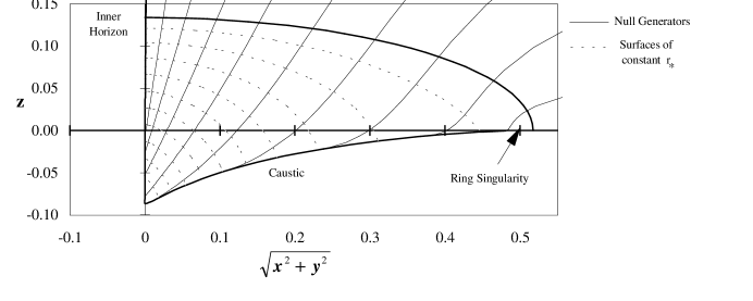
Figure 2: Null generators and surfaces of constant ${r_{\ast}}$ projected onto the Cartesian plane ($m=1,a=1/2$). This is a close-up of Figure 1 focusing on the region between the inner horizon and caustic. As in Figure 1 the northern half of the negative-$r$ sheet replaces the southern half of the positive-$r$ sheet to illustrate the evolution of the generators through the equatorial disk.

11 Concluding Remarks

Despite the complexity of the coordinate transformations linking them to the familiar Boyer-Lindquist coordinates, the quasi-spherical coordinates ${r_{\ast}}$, ${\theta_{\ast}}$ introduced in this paper and the light cones associated with them provide new and useful insights into the structure of the Kerr geometry and wave propagation in Kerr spacetime. We anticipate that they will find increasing use as their special advantages become apparent.

Acknowledgements This work was supported by NSERC of Canada and by the Canadian Institute for Advanced Research.

References

• [1] Wald RM 1984 General Relativity (Chicago IL: University of Chicago Press) p.223
• [2] Kerr RP 1963 Phys. Rev. Letters 11 237
• [3] Hawking SW and Ellis GFR 1973 The Large Scale Structure of Space-Time (Cambridge: Cambridge University Press) p.163
• [4] Boersma S and Dray T 1995 Gen. Rel. Grav. 27 319
• [5] Balasin H 1997 Class. Quantum Grav. 14 3353
Israel W 1977 Phys. Rev. D15 935
• [6] Keres H 1967 Soviet Physics JETP 25 504
Israel W 1970 Phys. Rev. D2 640
• [7] Ori A 1997 Gen. Rel. Grav. 7 881
• [8] Poisson E and Israel W 1990 Phys. Rev. D41 1796
• [9] see for example D’Inverno R 1996 Introducing Einstein’s Relativity (New York: Oxford University Press) p.261